Spatio-temporal variability of drought and effect of large scale climate in the source region of Yellow River

Abstract

The effects of drought, a devastating natural disaster, have expanded due to intense global warming. Therefore, studying the spatio-temporal evolution and formation mechanism of drought is urgent and important. In this paper, the standardized precipitation evapotranspiration index (SPEI) of the source region of Yellow River was calculated for the years 1961–2015, and the heuristic segmentation and Modified Mann-Kendall methods were used to study the change points and trends of precipitation, temperature, and SPEI. The empirical orthogonal function was used to study the major modes of the SPEI, and cross wavelet analysis was used to demonstrate the relationship between SPEI and large-scale climate factors. The results initially demonstrated no change point and an insignificant positive trend in precipitation. Temperature revealed a significant increasing trend, and a change point was detected in 1997. SPEI indicated a change point in 1993, and a significant increasing trend was observed thereafter. These findings reveal that drought in the study area is highly related to the El Niño-Southern Oscillation. The North Atlantic and Arctic oscillations caused similar impacts on drought. By comparison, changes in SPEI were slightly related to the Pacific decadal oscillation. These results provide useful information for evaluating drought changes in the study area, early warning of drought, and water resource management.

Keywords:

• Drought
• precipitation
• temperature
• SPEI
• large-scale climate factors

1. Introduction

Drought, which is generally defined as lower than normal utilization of water resources (Wilhite 2000), presents very serious effects. Determining the occurrence, intensity, and termination of drought is very difficult. The phenomenon is an important factor of economic and social problems and bring about ecological and environmental damage (Wilhite 2000; Hao and Singh 2015; Hao et al. 2016; Kogan et al. 2016; Huang et al. 2015a, 2016a). Climatic disasters account for 70% of all natural disasters, and drought accounts for 50% of these climatic disasters. Global annual drought-induced losses have reached as high as 6–8 billion dollars, and this phenomenon is the natural disaster that affects human most seriously (Wilhite 2000). Continuous global warming has intensified the global hydrological cycle and triggered extreme events, such as drought and flooding (Alan et al. 2003; Allan and Soden 2008; Yang and Yang 2012; Yang et al. 2015; Huang et al. 2017a). While global drought is gradually normalizing, as manifested by the continuous increase in occurrence, frequency, and intensity of extreme drought events, the effects of drought are becoming increasingly prominent and destructive (IPCC 2012).

Drought is a complicated and serious environmental problem. Many studies have proven that precipitation mode and temperature increases are factors contributing to drought intensity and frequency (Burke et al. 2006; Wanders and Wada 2015). Therefore, many scientists have studied drought, especially in terms of its monitoring and evaluation (Das et al. 2014; Kogan and Guo 2015; Xie et al. 2016; Kogan et al. 2017; Chen et al. 2017), spatial-temporal variation (Ganguli and Gangulya 2016; Zeleke et al. 2017), and prediction (Maity et al. 2016; Hao et al. 2017). Drought indices can be determined from the complicated interaction of hydroclimatologic parameters, which can be estimated according to the spatial scale, duration, frequency, and severity of the phenomenon (Wilhite 2000).

To estimate the severity of drought and improve risk management, scientists have proposed many definitions and relevant drought indices (Burke et al. 2006). Indices such as the Palmer drought severity index (PDSI) (Palmer 1965), crop moisture index (CMI) (Palmer 1968), standardized precipitation index (SPI) (McKee et al. 1993), nonparametric multivariate standardized drought index (NMSDI) (Huang et al. 2015b), multivariate integrated drought index (MIDI) (Chang et al. 2016), and soil moisture deficit index (SMDI), have been proposed. Of these indicators, PDSI and SPI are the most highly utilized. PDSI is considered as a milestone in the development of drought indices and one of the most popular indices used today. However, this index presents some limitations, including a fixed time scale, poor performance in short-term drought events, and failure to explain physical phenomena in terms of spatial mode (Alley 1984). As an alternative, SPI is extensively used in drought research (Sierra-Soler et al. 2016; Huang et al. 2017b) due to its characteristics of simple calculation, calculation on various time scales, and strong adaptation to different climates. Calculation of SPI is based only on precipitation data, which means the index is especially suited to meteorological drought. However, while undoubtedly helpful, these indices do not consider other factors influencing drought, such as temperature, evapotranspiration volume, wind speed, and soil water-holding capacity (Vicente-Serrano et al. 2010). Thus, the standardized precipitation evapotranspiration index (SPEI) was proposed to integrate the advantages of the PDSI and SPI; this index not only considers the water-heat equilibrium process but also presents the characteristics of multiple time scales, simple calculation, and convenient data collection. SPEI is especially applicable when testing, monitoring, and exploring the influences of global warming on drought (Vicente-Serrano et al. 2010).

Many studies have demonstrated that drought is closely related to climatic indices, such as the El Niño-Southern Oscillation (ENSO), the North Atlantic oscillation (NAO), the Pacific decadal oscillation (PDO), and the Arctic oscillation (AO) (Mantua et al. 1997; Talaee et al. 2014; Huang et al. 2016b). ENSO is the major source of inter-annual global and regional climate changes. Ryu et al. (2010) discussed the correlation between drought in the United States of America and ENSO and found a negative correlation between droughts in Southern California and the northern part of the Great Plain and ENSO; a positive correlation between ENSO and drought in the northwest Pacific Ocean was also discovered. As an important component of atmospheric variability in the Northern Hemisphere, NAO influences the high-/middle-latitude continental climate by adjusting heat and water transportation (Hurrell 1995). Singh et al. (2015) analysed the coupled effects of ENSO-PDO, ENSO-AMO, and ENSO-NAO on base flow and revealed that ENSO-PDO can markedly affect base flow interactions. In particular, the occurrence of La Niña during the positive phase of PDO reduces base flows significantly, causing serious drought in the Apalachicola-Chattahoochee-Flint River Basin.

China belongs to a continental climate region that experiences violent climatic fluctuations. Social economy, food safety, ecology, and the environment rely highly on climate conditions. China suffers serious and frequent drought events, and the superposed impacts of the East Asian tropical and subtropical monsoon climates markedly affect the country. Global warming brings about continuous changes in these two monsoon climates, thereby influencing the spatial layout and development trend of droughts. Thus, studying the spatio-temporal characteristics of droughts is of great significance in water resource management, especially in China.

The Tibet Plateau, the largest plain in China, possesses a unique natural environment; it is also the headstream of the country’s major rivers, including Yangtze River, Yellow River, Yarlung Zangbo River, Lancang River, and Nujiang River. The source region of Yellow River (YRS) lies in the transition zone between the Tibet Plateau and Loess Plateau. Besides being an ecological shelter zone and providing water to the Yellow River Basin, this region is also a vulnerable ecological environment and highly sensitive to climate changes (Chang et al. 2016, 2017). Climate changes and drought in the YRS play an important role in the sustainable development of social economy in China. Although many studies on the phenomenon are available, research on the distribution, variation trend, and responses of droughts to general large-scale ocean-atmosphere circulation patterns in the YRS in China is highly limited.

The research goals of this paper are: (1) to examine spatial-temporal changes in precipitation, temperature, and drought indices in the YRS, (2) to analyse the distribution characteristics of SPEI in the source region, and (3) to determine whether a significant antecedent relationship exists between drought indices and large-scale climate factors. This study presents several novel concepts: (1) Previous studies mainly evaluate droughts in terms of the spatial distribution of SPEI. In this paper, SPEI distribution is studied using the empirical orthogonal function (EOF), and the distribution characteristics of drought are disclosed. (2) The relationship between two time series is generally studied through correlation coefficients. However, cross wavelet analysis can comprehensively disclose relationships in both the time and frequency ranges. The remainder of this paper is organized as follows. Section 2 describes the study area and available data, Section 3 introduces the research methodology, Section 4 analyses the results, Section 5 presents the discussion, and Section 6 provides the conclusions.

2. Study area and materials

2.1. Study area

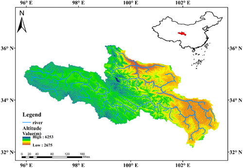
In this paper, the YRS refers to the river basin above the Tangnaihai hydrologic station. It is located northeast of the Tibet Plateau and considered a major water production area (Figure 1). The study area has an altitude of 2700–6300 m and lies between the eastern longitude of 95.7°–103.8° and the northern latitude of 31.7°–36.3°. The study area is a typical plateau with a continental semi-arid climate. Influenced by monsoon climates, the annual precipitation in this region is 331–989 mm. The time distribution of precipitation is uneven and manifested by low precipitation in spring and winter but high precipitation in summer and autumn (from June to September). The annual average temperature ranges from −7.0 °C to 2.7 °C, and precipitation and temperature decrease gradually from southeast to northwest.

Figure 1. Location of the source region of Yellow River.

2.2. Study data

Monthly precipitation and temperature data from 1961 to 2015 were collected from the China Meteorological Data Network of China Meteorological Administration (CMA). All of the data were gridded with a horizontal resolution of 0.5° × 0.5° and then subjected to spatial interpolation by using thin plate splines (TPS) based on the latest compilation of precipitation data of the China Ground 2472 Station of the National Meteorological Information Centre. Cross verification and error analysis indicated that the data were of high quality. In this paper, grids had a reasonable spatial coverage range and were distributed close to the edges of the internal and external source regions of Yellow Source. Less than 0.05% of the data of the study area were missing; these data were replaced by the mean value of the data of multiple years in the same months. Such replacement is adequate to study spatio-temporal distributions and variations in climatic elements and drought indices, which is one of the research goals of this paper.

In this paper, the relationship between SPEI in the YRS and large-scale ocean-atmosphere general circulation pattern, including ENSO, NAO, PDO, and AO, is discussed. ENSO can be expressed by several indices, which include the Southern oscillation index (Ward et al. 2016), NINO l, NINO 3, NINO 3.4, and multiple ENSO index (MEI). In this paper, MEI was used because it integrates more information than other indices (Limsakul and Singhruck 2016). MEI data can be downloaded from http://www.esrl.noaa.gov/psd/enso/mei/table.html. Monthly NAOI data were collected from https://climateataguide.ucar.edu/climate-data/hurrell-north-atlantic-oscillation-nao-index-pc-based. PDO was defined as the major component of the monthly rate of sea-surface temperature change in the North Pacific Ocean, and PDO data were collected from the Tokyo Climate Center (ds.data.jma.go.jp/tcc/tcc/products/elnino/decadal/annpdo.txt). AO data were obtained from the NOAA (www.ncdc.noaa.gov/teleconnections/ao/).

3. Methodology

3.1. SPEI

SPEI is a multi-component drought index that is based on precipitation and potential evapotranspiration (PET) and sensitive to global warming. It describes the deflection degree of dry and wet conditions according to standardized PET and precipitation (Vicente-Serrano et al. 2010). Since SPEI can capture the drought characteristics of different time scales (1, 3, 6, 12, and 24 months), it is widely used in drought evaluation. SPEI is calculated by combining the calculations of PDSI and SPI; a detailed calculation process for SPEI is provided by Vicente-Serrano et al. (2010).

3.2. Heuristic segmentation

Change points of the meteorological factors and time series of SPEI must be examined to determine whether they are stable. Several methods may be used to detect breakpoints in climate, including the moving $t$-test, sum of ranks, and Mann-Kendall (MK) test. Bernaola-Galván et al. (2001) proposed the method of heuristic segmentation, which is based on the moving$\mathrm{ }t$-test but modified to divide non-stationary series into several fixed sequences, thus overcoming the shortages of the above methods. Statistical${\mathrm{ }T}_{(i)}$ values at each point are calculated according to the t-test, after which the statistical significance $P_{(T_{max})}$ of the maximum value $T_m$ in $T_{(i)}$ is calculated. A change point is determined when $P_{(T_{max})}$ is higher than the critical value $P_0$. If a change point exists in the time series, each new time series is continuously segmented (i.e., the second iteration and segmentation process, the third iteration and segmentation process, and so on) until the limited length of time series is smaller than the pre-set minimum segmented length ($l_0$). Generally speaking, the value of${\mathrm{ }l}_0$ is smaller than 25 and $P_0$ can be valued 0.5–0.95. According to the data, the thresholds of $l_0$ and $P_0\mathrm{ }$were set to 25 and 0.90, respectively.

3.3. Modified Mann–Kendall trend analysis

Trends of meteorological elements and SPEI time series were tested. The original MK trend test is a nonparametric test recommended by the World Meteorological Organization (Mitchell et al. 1966). However, this test is based on the hypothesis of sequence independence. Here, the sequence is significantly underestimated in case of negative correlation and significantly overestimated in case of positive correlation (Hamed and Rao 1998; Hamed 2008). To eliminate the influences of continuity, Hamed and Rao (1998) proposed an estimation of the autocorrelation coefficient ${\rho }_i$ of a new time series by extracting the non-parameter trend estimation series from the original time. Modified MK trend analysis (MMK) can better capture the trend of hydrologic sequences compared with its original form (Daufresne et al. 2009).

The variance of revised statistics S is Var* (S): (1) $${\text{Var}}^{*} \left(\mathrm{S}\right)=\text{Var}\left(\mathrm{S}\right)\cdot \eta$$(1)

where $\mathrm{\eta }=1+\frac{2}{N\left(N-1\right)\left(N-2\right)}{\sum }_{i=1}^{N-1}\left(N-i\right)\left(N-i-1\right)\left(N-i-2\right){\rho }_i$.

3.4. EOF analysis

The EOF, also known as eigenvector analysis, was proposed by Person (1901). It is applicable to fields where spatial points (multiple variables) use grid point changes over time. The function is used to represent raw data based on a series of orthogonal basis functions and correlation coefficients. The method was first introduced to meteorology and then used extensively by oceanologists and meteorologists.

The variable matrix is, (2) $$X_{mn}=V_{mn}{T}_{mn}$$(2)

where $V_{mn}$ and $T_{mn}$ are function matrices of space and time, respectively, $m$ and $n$ are the values of the space points and time series, respectively.

The purpose of EOF analysis is to find the eigen values and eigen functions of the variable matrix. The function has many advantages, including no fixed function, quick convergence, and decomposition of irregularly distributed stations (Wei 2007). Dvinskikh (1988) provides more details of the EOF. The first EOF was chosen as the pattern that is most frequently realized. Then, the second mode is the most commonly realized pattern under the constraint of orthogonality to the first pattern, the third mode is the most frequently realized pattern orthogonal to the two higher modes, and so on (Zerbini 2010). North (1982) revealed that a significance test is necessary to determine whether the results of EOF decomposition are significant. In this paper, spatial analysis of the YRS was carried out through EOF.

3.5. Cross wavelet analysis

Wavelet analysis can determine the temporal frequency characteristics of time series; thus, it is an effective tool for analysing time series. Cross wavelet analysis combines the features of wavelet transformation and cross spectral analysis. Compared with Fourier transformation, cross wavelet analysis can better reflect variation features and coupled oscillation of the time-frequency domains of two time series (Hudgins et al. 1993; Hudgins and Huang 1996; Torrence and Compo 1998). Because cross wavelet analysis may not be completely localized in time, the cone of influence (COI) was introduced as one region to overcome this limitation (Grinsted et al. 2004). Cross wavelet transformation presents strong signal coupling and resolution ability, and it can easily describe the distribution patterns and phase relations of coupled signals in the time–frequency domain (Maraun and Kurths 2004; Dong et al. 2013). Relevant codes can be downloaded for free from http://www.pol.ac.uk/home/research/waveletcoherence/. In this paper, cross wavelet analysis was used to analyze the remote relationships between drought indices and large-scale climatic factors in the study area.

4. Results

4.1. Possible change points of precipitation, air temperature, and SPEI

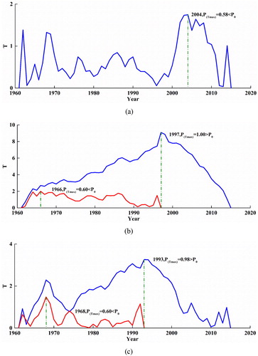
Climate changes (global warming) and anthropogenic activities (e.g. construction of water conservancy projects) have influenced the study area significantly. Possible change points of precipitation, temperature, and SPEI time series were determined by heuristic segmentation, and the results are shown in Figure 2. As shown in Figure 2(a), $T_m$ of precipitation was observed in 2004, but this finding failed the significance test. In Figure 2(b), the $T_m$ value of temperature peaked in 1997 and $P_{(T_{max})}$ was 1, indicating a change point in temperature. This result has been verified by other studies (Lan et al. 2013; Li et al. 2012). No change point was detected in the second segmentation, which means temperature underwent only one change point (1997) during the study period. Figure 2(c) shows that the $P_{(T_{max})}$ of the time series of SPEI (0.94) was achieved in 1993; the value of this parameter is higher than the threshold ($P_0$). A change point (1993) in the SPEI time series was identified, but, in the second iteration, $P_{(T_{max})}$ failed the significance test. Thus, only one change point was detected in the time series of SPEI.

Figure 2. Segmentations and change points of precipitation, temperature, and SPEI in the source region of Yellow River (red line, the first iteration and segmentation process; blue line, the second iteration and segmentation process).

Figure 2 Segmentations and change points of precipitation, temperature, and SPEI in the source region of Yellow River (red line, the first iteration and segmentation process; blue line, the second iteration and segmentation process).

4.2. Changes in precipitation, air temperature, and SPEI

The spatial distribution and variation trends of precipitation, temperature, and SPEI in the study area are shown in Figure 3. Figure 3(a) shows the spatial distribution of annual average precipitation and variation trend of different grid points in the study area from 1961 to 2015. As shown in Figure 3(a), precipitation increased from northwest to southeast, and the maximum precipitation was concentrated in the southeastern portion of the river basin. This finding was determined from the geological characteristics of the study area. The Bay of Bengal is the main source of water vapour in the study area, and the path of water vapour transmission in the Tibet Plateau influences the spatial distribution of precipitation. Regions with low precipitation are regions with a vulnerable ecology/environment. Most grids (56.86% of the total grids) presented insignificant positive trends. By comparison, 19.61% of the total grids showed significant increasing trends. The proportion of grids with insignificant negative trends was 23.53%. In general, precipitation in the study area increased gradually, but the positive trend was not significant. This finding conforms to other research results (Wang et al. 2006; Li et al. 2012; Lan et al. 2016).

Figure 3. Spatial distributions and variation trends of (a) precipitation, (b, c) temperature, and (d, e) SPEI in the study area.

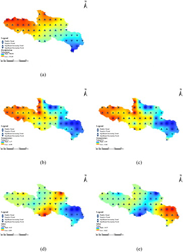
The spatial distribution and variation trend of annual average temperature in the study area from 1961 to 1997 are shown in Figure 3(b). Similar to precipitation, temperature generally increased from northwest to southeast, which means temperature is highly related to altitude. Grids with significant increasing trends and insignificant positive trends accounted for 58.82% and 23.53% of the total grids, while grids with significant decreasing trends accounted for 3.92% of the total. The distribution of and changes in annual average temperature from 1998 to 2015 are shown in Figure 3(c). In terms of spatial distribution, the temperature was generally higher than that in 1961–1997. The highest temperature was found southeast of the study area, while the lowest temperature was observed in the northwest. The proportions of grids with significant increasing and decreasing trends were 90.20% and 1.96%, respectively. The proportion of grids with significant increasing trends dramatically increased after 1997, indicating a large-scale temperature increase in the study area. Overall, the temperature significantly increased from southeast to northwest in 1961–2015, in accordance with previous study results (Li et al. 2012; Lan et al. 2016). Temperature presented similar spatial distributions in the study area in 1961–1997 and 1961–1997.

Variations in SPEI in the study area from 1961 to 1993 are presented in Figure 3(d). In terms of spatial distribution, the southern regions of the study area suffered relatively serious drought, while the eastern region experienced slight droughts. In terms of variation trend, the proportions of grids with insignificant negative trends and significant increasing trends were the highest (39.22%) and the lowest (5.88%), respectively. In general, SPEI remained stable from 1961 to 1993. As shown in Figure 3(e), the southern regions of the study area experienced the least severe drought from 1994 to 2015; by contrast, the eastern regions suffered serious droughts. The centre of drought was altered compared with that in the drought distribution before 1993. SPEI in the study area increased continuously from 1994 to 2015. Specifically, the proportion of grids indicating a significant increasing trend reached 43.14%, and the proportion of grids indicating an insignificant positive trend reached 50.98%. This result implies that the study area had become wetter in recent years.

4.3. EOF analysis

EOF analysis of SPEI over a 12-month scale using grids in the study area from 1961 to 2015 was carried out. The first four modes were selected to analyse spatial and temporal changes. Modes 1, 2, and 4 passed the North test, and the cumulative variance of the contribution rates reached 85.91%, indicating good convergence. Moreover, the first four modes demonstrated outstanding physical significance and could reflect the major distribution features of SPEI in the study area (Figure 4).

Figure 4. Distribution of the first four modes gained from EOF analysis.

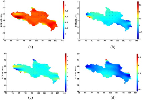
The first mode of the EOF was the main drought distribution feature in the study area. The variance of the contribution rate of the first mode was 62.18%, and the spatial distribution of this mode that all components was consistently negative. This result indicates that the same variation trend of SPEI is the major feature of the study area in 1961–2015. In other words, the YRS will be overall drier or overall wetter. The second mode of EOF showed a positive-negative alternating distribution that was mainly negative in the east and positive in the west. When the positive region was in a dry state, the negative region was wet, and vice versa. The variance of the contribution rate of this mode was 12.13%. The maximum positive value was found east of the study area, and the minimum negative values were found west of the study area. Northwest of the basin, a large negative value appears, and the area is close to another area with the largest positive value area. Furthermore, the maximum positive value occurred in high-altitude regions and the minimum negative value occurred in low-altitude regions, thus indicating the significant impacts of altitude on mode distribution. The third mode of EOF also revealed a positive–negative alternating pattern, and the variance of the contribution rate of the third mode was 6.29%. The largest negative value appeared in the western portion of the study area, while the largest positive value appeared in the southwest. The fourth mode of EOF demonstrated a positive-negative alternating distribution; this mode was positive in the middle regions of the study but negative in the northwestern and eastern regions. The variance of the contribution rate of this mode was 5.31%.

4.4. Correlations between the large-scale climatic factors and SPEI in the YRS

Global observations indicate that large-scale climatic factors are closely related to drought. Changes in global ocean temperature or large-scale climate factors (e.g. ENSO, NAO, PDO, and AO) may be crucial to the formation of drought on the inter-decadal scale (Talaee et al. 2014; Zhang et al. 2015). Studying the relationships among these factors, especially the evolution of these relations, can help improve the current understanding on drought changes, which is of significance to drought warning and water resource management. In this work, cross wavelet analysis was used to study the relationships between drought and large-scale climate factors (ENSO, NAO, PDO, and AO) (Figure 5).

Figure 5. Cross wavelet transformation of SPEI and large-scale climatic factors from 1961 to 2015: (a) ENSO, (b) NAO, (c) PDO, (d) AO.

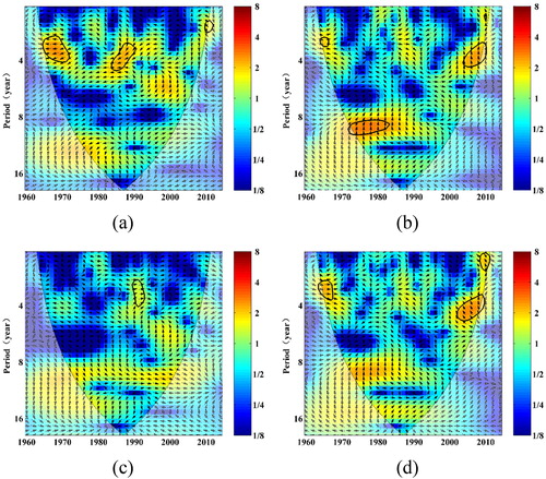
The results of cross wavelet transformation between SPEI and climatic factors in the study area are shown in Figure 5; here, arrows reflect the phase relationship between factors. The arrow pointing from left to right indicates positive associations, while the arrow pointing from right to left indicates negative correlations. Upward- or downward-pointing arrows, respectively, reflect drought behind or ahead of the climate index by 1/4 cycle and reveal a nonlinear correlation. The values enclosed by the thick black solid lines pass the red noise test at the 95% confidence level. The thin black solid line envelopes the COI, that is, the region is highly influenced by the marginal effect of data during continuous wavelet transformation, and the right-hand coloured stripes represent wavelet energies.

As shown in Figure 5(a), the COI, SPEI, and MEI were significantly correlated at the 95% confidence level. In 1965–1973 and 1984–1991, signals of 2.96–4.10 and 3.23–4.55 years, were respectively observed. A statistically negative correlation between these variables was found. The results indicate that ENSO events play an important role in drought in the YRS. In 1965–1967, SPEI and NAO revealed a signal of 3.01–3.39 years at the 95% confidence level, and a statistical positive correlation was found. Signals of 8.32–9.98 and 3.21–4.34 years in the respective periods of 1974–1984 and 2001–2010 were also revealed. As shown in Figure 5(c), a signal of 2.92–4.08 years could be observed from 1990 to 1994, and SPEI was positively correlated with PDO. In Figure 5(d), SPEI and AO signals of 2.95–3.76 years could be found in the period 1965–1968, and a statistically positive correlation between these variables was observed.

As shown in Figure 5, ENSO, NAO, and AO are more strongly correlated with SPEI than with PDO, thus indicating that drought in the study area is only slightly influenced by PDO. This finding, however, may be restricted by a relatively short recording length and uncertain potential interactions between PDO and ENSO (Kiem and Verdon-Kidd 2009). Precipitation and temperature are the input factors of SPEI, and PDO can indirectly influence the change rate of precipitation by adjusting ENSO (Verdon et al. 2004).

5. Discussion

To further study the non-stationary nature of SPEI, the inter-annual variation and annual mean of SPEI were calculated (Figure 6). Temporal changes in SPEI are shown in Figure 6. SPEI clearly only had one change point in 1993 according to the results in Section 4.2. The annual means of SPEI in the periods of 1961–1993 and 1994–2015 were 0.31 and –0.45, respectively. According to drought levels (Table 1, modified from McKee et al. 1993), the study area was wet before 1993 but experienced mild drought after 1993.

Figure 6. Comparison of the time series before (solid blue line) and after (solid red line) the change point of SPEI in the source region of Yellow River. The solid black line represents the annual SPEI time series.

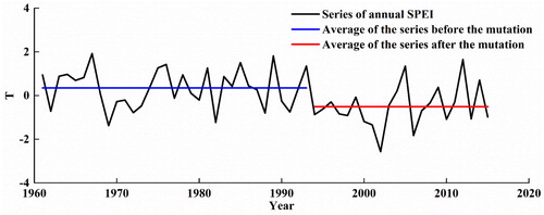
Table 1. Classification of drought according to SPEI.

Level	Drought class	SPEI value
1	Mild drought	0.00 to −0.99
2	Moderate drought	−1.00 to −1.49
3	Severe drought	−1.50 to −1.99
4	Extreme drought	≤ −2.00

Cross wavelet transformation cannot disclose the low-energy regions of two time series in the time-frequency domain, but this limitation can be offset by cross wavelet coherence analysis (Adamowski and Prokoph 2013). To further explore the remote correlation between SPEI and large-scale climate factors, the correlation between these items in low-energy regions under different time scales is shown in Figure 7. As shown in Figure 7(a), in 1964–1984, SPEI and ENSO showed higher energies lasting about 2.72–5.03 years. The phase difference observed demonstrated that SPEI and ENSO were negatively correlated in this period as the arrows point from right to left. As shown in Figure 7(b), during the period of 1966–1969, SPEI and NAO had high energies lasting about 3.01–5.02 years. SPEI exhibited a statistically significant positive correlation with NAO. In the period of 2004–2009, SPEI and NAO had high energies lasting about 2.06–4.74 years, and the variability of SPEI lagged behind that of NAO. Nevertheless, the correlation between SPEI and NAO in 1974–1983 failed the significance test. Outside of the COI, a period of high energies lasting 10.88–13.09 years was observed in 1962–1975 between SPEI and NAO. A significant resonance relationship is found in this frequency band, and the oscillation observed is cohesive. Similarly, SPEI also lagged behind NAO. In Figure 7(c), SPEI and PDO had high energies lasting approximately 3.96–5.33 and 7.19–9.48 years in the periods 1968–1978 and 1971–1980, respectively. Note that although the periods of influence of these two signals were close, their spheres of influence were different. SPEI showed a statistically significant negative correlation with PDO, and the variability of PDO lagged behind the variability of SPEI. According to Figure 7(d), the respective resonance periods of SPEI and AO in the periods 1965–1970 and 2003–2009 were 2.86–5.19 and 3.88–7.80 years, respectively.

Figure 7. Cross wavelet coherence spectra between SPEI and large-scale climatic factors during the period of 1961–2015: (a) ENSO, (b) NAO, (c) PDO, (d) AO.

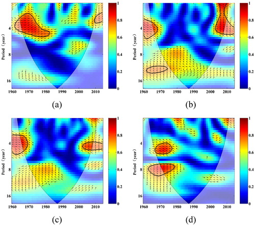
As shown in Figure 5(a), the annual SPEI has a significantly negative correlation with ENSO events in the periods of 1965–1973 and 1984–1991. Figure 7(a) reveals a strong negative correlation between SPEI and ENSO in 1964–1984 at the 95% confidence level. Generally, ENSO events are closely associated with droughts in the YRS, which implies that this process increased the drought level in the area. As shown in Figures 5(b) and 7(b), a positive correlation existed between SPEI and NAO in the periods of 1965–1967 and 1966–1969 in the high- and low-energy regions, respectively These findings confirm the associations between SPEI and NAO and imply that NAO decreased drought conditions in the YRS. While Figure 5(c) shows a strong negative correlation between SPEI and PDO in 1990–1994, Figure 7(c) exhibits a significant positive correlation between these indices in 1968–1978. This result shows that PDO has an important effect on SPEI, but this effect varied at different periods. Such a change trend could lead to phase changes in the relationship of these indices during the two periods cited, likely because drought is affected not just by AO but also by other factors, such as the underlying surface and anthropogenic activities. In earlier years, the study area featured a mild wet state; in later years, however, the YRS transformed from wet to mildly dry. A statistically significant positive correlation between SPEI and AO in 1965–1968 and 1965–1970 was observed in the high-energy and low-energy regions, respectively, as shown in Figures 5(d) and 7(d). This result implies that PDO exerts a strong influence on droughts, specifically decreasing drought conditions in study area. NAO and AO demonstrated similar time ranges and periods with SPEI in the high- and low-energy regions, thus indicating their similar influences on drought in the study area. In conclusion, ENSO, NAO, PDO, and AO are closely associated with drought conditions and exert strong influences on the climate in the study area.

ENSO is formed by large-scale ocean-atmosphere interactions that intensify the occurrence of extreme hydrological climate events, such as flood, drought, and hurricane (Cole and Cook 1998; Andrews et al. 2004; Zhang et al. 2007, 2013). Wang et al. (1999) confirmed the occurrence of an ENSO event in 1867–1998, including a warm event that lasted for three seasons in 1993 and a warm event that lasted for five seasons in 1997–1998. According to the calculation results of heuristic segmentation, the temperature in the study area showed a change point in 1997 when the warm event of ENSO occurred. A warm event occurred in 1993, during which a change point was also observed in the time series of SPEI. These findings further prove the significant influences of ENSO on temperature and SPEI in the study area.

ENSO and PDO are climatic phenomena formed by ocean–atmosphere interactions in the equatorial Pacific and North Pacific Ocean regions. They can influence energy flow in the Pacific Ocean and affect the climate in other regions through global atmospheric circulation. The YRS is located in the interaction belt of the southeast and southwest monsoons, and energy fluctuations in the Pacific can influence precipitation and temperature changes in the region. According to Beebee and Manga (2004), ENSO is highly correlated with changes in annual runoff, while PDO is strongly correlated with the snow melting time. Glaciers may be found in the YRS, and PDO could influence the glacier melting time, thereby affecting drought changes in the region. PDO affects the sea-level pressure in the Asian monsoon region through sea interactions and interacts with changes in land pressure to affect water vapour transport, precipitation, and drought.

NAO is the main source region of inter-annual climatic variation in the Northern Hemisphere (Hurrell and Van Loon 1997); it influences the westerlies, thereby affecting vapour transmission and radiation above the Tibet Plateau. Therefore, NAO influences precipitation in the study area and changes in SPEI. In the middle latitude, NAO and AO reflect the strength of the westerlies, which cause important and extensive impacts on climatic changes in the Northern Hemisphere. Fluctuations in NAO and AO significantly influence climatic factors, such as air temperature, precipitation, and snow cover. Cross wavelet analysis revealed that the occurrence and periods of signals of NAO and AO in high-energy and low-energy regions are similar and that NAO has stronger impacts than AO.

Global climatic changes have brought about increased attention to drought events. Yu et al. (2014) pointed out that serious and extreme drought events have become increasingly frequent in China since the late 1990s. By contrast, the eastern regions of the Tibet Plateau have experienced significant wetting. Cook et al. (2010) studied climatic changes of the “third pole” and concluded that eastern regions of the Tibet Plateau are becoming increasingly wet mainly because of melting of the Himalayan glaciers as a response to global warming. Xu et al. (2015) studied drought in China using SPI, SDI, and SPEI and recognized an increasing wetting trend in the Tibet Plateau. The YRS lies in the eastern portion of the Tibet Plateau, and a significant wetting trend was observed during the period of 1993–2015, which conforms to the findings of Xu et al. Global warming has caused marked temperature increases in the study area accompanied by PET growth and insignificant precipitation. Temperature increases induce strong melting and shrinkage of glaciers, and water from melted glaciers can increase soil water contents and river runoff. These events may explain the increasing wetting trend in the study area.

Temperature changes in the study area can influence the local frozen earth distribution, ecological environment, and hydrologic processes. Given significant increases in temperature, degradation of permanently frozen soil may be observed (Yang et al. 2010). Degradation of this soil can cause groundwater recession, gradual shrinkage of lakes and wetlands, and intensified desertion and soil erosion. The carbon released can accelerate global warming (Jin et al. 2009; Yang et al. 2010). Ecological–hydrological processes in the study area can change as a result of degradation of frozen soil (Qin et al. 2017). Regional drought may cause ecological degradation, reduction of vegetable coverage, and water and soil loss, thereby influencing vapour circulation and human social production. The study area presented a warm and wet trend after 1993, which would relieve the negative impacts of drought to some extent, improve the local hydrological system and ecological environment, and even facilitate sustainable development.

In this paper, the SPEI in the study area was calculated using precipitation and air temperature data, and spatial-temporal variations in precipitation, air temperature, and SPEI were analysed. The correlations between SPEI and large-scale climate factors were discussed, and annual changes in drought in the study area were studied. The relationships between SPEI time series and climatic factors when the drought threshold is negative require further study. Drought analysis under different time scales, as well as analysis of drought frequency, drought intensity, and drought duration, should be studied further.

6. Conclusions

Studying the distribution, evolution patterns, and causes of drought can help disclose the response mechanisms of drought to environmental changes, which is of extremely important significance to drought relief. In this paper, change points in the time series of precipitation, temperature, and SPEI in the study area during the period of 1961–2016 were discussed. The distribution characteristics of the SPEI were analysed using the EOF technique, and possible correlations between drought and large-scale climatic factors were studied by cross wavelet analysis. The major conclusions of this work are as follows:

1. No change point was found in the time series of precipitation in the study area. However, in the time series of temperature and SPEI, change points were identified in 1997 and 1993, respectively.

2. Precipitation generally increased during the study period, but the positive trend observed was insignificant. In general, the temperature revealed a significant increasing trend over the study period. Noticeable increasing trends of temperature were observed in 1961–1997 and 1998–2015. Overall, SPEI exhibited a negative trend throughout the study period; it remained basically stable in 1961–1993 but showed a significant increasing trend in 1994–2015, indicating a wetting trend in the study area over the last two decades.

3. The major variation characteristics of the time series of SPEI were basically consistent and showed good convergence. The regional altitude influenced the drought distribution in the study area.

4. Cross wavelet analysis revealed that ENSO, NAO, PDO, and AO are closely associated with the occurrence and variability of drought in the YRS, although the extent of influence and signal periods differed from one index to another.

Acknowledgments

We express our sincere thanks to the Editor and reviewers for their valuable comments.

Disclosure statement

No potential conflict of interest was reported by the authors.

Additional information

Funding

This work was supported by the National Natural Science Foundation of China under Grant No. 51509202 and the National Key R&D Program of China under Grant No. 2017YFC0403600.

References

- Adamowski J, Prokoph A. 2013. Determining the amplitude and timing of stream flow discontinuities: a cross wavelet analysis approach. Hydrol Proc. 28:2782–2793. doi:10.1002/hyp.9843.
- Alam NM, Sharma GC, Moreira E, Jana C, Mishra PK, Sharma NK, Mandal D. 2017. Evaluation of drought using SPEI drought class transitions and log-linear models for different agro-ecological regions of India. Phys Chem Earth 100:31–43.
- Alan DZ, Justin S, Edwin PM, Bart N, Eric FW, Dennis PL. 2003. Detection of intensification in global- and continental-scale hydrological cycles: temporal scale of evaluation. J Clim. 16:535–547.
- Allan RP, Soden BJ. 2008. Atmospheric warming and the amplification of precipitation extremes. Science 321(5895):1481–1484.
- Alley WM. 1984. The Palmer Drought Severity Index: limitations and assumptions. J Climate Appl Meteor. 23(7):1100–1109.
- Andrews ED, Antweiler RC, Neiman PJ, Ralph FM. 2004. Inflence of ENSO on flood frequency along the California coast. J Climate. 17:337–348.
- Bernaola-Galván P, Ivanov PC, Amaral LAN, Stanley HE. 2001. Scale invariance in the nonstationarity of human heart rate. Phys Rev Lett. 87(16):168105.
- Burke EJ, Brown SJ, Christidis N. 2006. Modeling the recent evolution of global drought and projections for the twenty-first century with the Hadley Centre climate model. J Hydrometeor. 7(5):1113–1125.
- Chang JX, Li YY, Wang YM, Yuan M. 2016. Copula-based drought risk assessment combined with an integrated index in the Wei River Basin, China. J Hydrol. 540:824–834.
- Chang JX, Li YY, Yuan M, Wang YM. 2017. Efficiency evaluation of hydropower station operation: a case study of Longyangxia Station in the Yellow River, China. Energy. 135:23–31.
- Chang JX, Zhang HX, Wang YM, Zhu YL. 2016. Assessing the impact of climate variability and human activities on streamflow variation. Hydrol Earth Syst Sci. 20(4):1547–1560.
- Chen CF, Son NT, Chen CR, Chiang SH, Chang LY, Valdez M. 2017. Drought monitoring in cultivated areas of Central America using multi-temporal MODIS data. Geomat Nat Haz Risk. 8(2):402–417.
- Cole JE, Cook ER. 1998. The changing relationship between ENSO variability and moisture balance in the continental United States. Geophys Res Lett. 25(24):4529–4532.
- Cook ER, Anchukaitis KJ, Buckley BM, D’Arrigo RD, Jacoby GC, Wright WE. 2010. Asian monsoon failure and megadrought during the last millennium. Science 328:486–489.
- Das PK, Murthy CS, Seshasai MVR. 2014. Monitoring of seasonal dryness/wetness conditions using shortwave angle slope index for early season agricultural drought assessment. Geomat Nat Haz Risk. 5(3):232–251.
- Daufresne M, Lengfellner K, Sommer U. 2009. Global warming benefits the small in aquatic ecosystems. Proc Natl Acad Sci USA 106(31):12788–12793.
- Dong LY, Chen JY, Fu CS, Jiang HB, Yang XY. 2013. Recognition on the relationship between runoff and regional meteorological factors of the Xijiang River in multi-time scales. Scientia Geograpnica Sinica. 33(2):209–215.
- Dvinskikh NI. 1988. Expansion of ionospheric characteristics fields in empirical orthogonal functions. Adv Space Res. 8(4):179–187.
- Ganguli P, Ganguly AR. 2016. Space-time trends in U.S. meteorological droughts. J Hydrol. 8:235–259.
- Grinsted A, Moore JC, Jevrejeva S. 2004. Application of the cross wavelet transform and wavelet coherence to geophysical time series. Nonlin Processes Geophys. 11(5/6):561–566.
- Hamed KH, Rao AR. 1998. A modified Mann-Kendall trend test for autocorrelated data. J Hydrol. 204(1–4):182–196.
- Hamed KH. 2008. Trend detection in hydrologic data: The Mann–Kendall trend test under the scalinghypothesis. J Hydrol. 349:350–363.
- Hao ZC, Hao FH, Singh VP. 2016. A general framework for multivariate multi-index drought prediction based on multivariate ensemble streamflow prediction (MESP). J Hydrol. 539:1–10.
- Hao ZC, Singh VP. 2015. Drought characterization from a multivariate perspective: A review. J Hydrol. 527:668–678.
- Hao ZC, Xia YL, Luo LF, Singh VP, Wei OY, Hao FH. 2017. Toward a categorical drought prediction system based on U.S. Drought Monitor (USDM) and climate forecast. J Hydrol. 551:300–305.
- Huang SZ, Huang Q, Chang JX, Chen YT, Xing L, Xie YY. 2015. Copulas-based drought evolution characteristics and risk evaluation in a typical arid and semi-arid region. Water Resour Manage. 29(5):1489–1503.
- Huang SZ, Huang Q, Chang JX, Leng GY. 2016a. Linkages between hydrological drought, climate indices and human activities: a case study in the Columbia River basin. Int J Climatol. 36(1):280–290.
- Huang SZ, Huang Q, Chang JX, Zhu YL, Leng GY, Xing L. 2015b. Drought structure based on a nonparametric multivariate standardized drought index across the Yellow River basin. China. J Hydrol. 530:127–136.
- Huang SZ, Huang Q, Leng GY, Liu SY. 2016. A nonparametric multivariate standardized drought index for characterizing socioeconomic drought: a case study in the Heihe River Basin. J Hydrol. 542:875–883.
- Huang SZ, Leng GY, Huang Q, Xie YY, Liu SY, Meng EH. 2017a. The asymmetric impact of global warming on US drought types and distributions in a large ensemble of 97 hydro-climatic simulations. Sci Rep. 7(1):5891.
- Huang SZ, Li P, Huang Q, Leng GY, Hou BB, Ma L. 2017. The propagation from meteorological to hydrological drought and its potential influence factors. J Hydrol. 547:184–195.
- Hudgins L, Friehe CA, Mayer ME. 1993. Wavelet transforms and atmospheric turbulence. Phys Rev Lett. 71(20):3279–3282.
- Hudgins L, Huang JP. 1996. Bivariate wavelet analysis of Asia Monsoon and ENSO. Adv Atmos Sci. 13(3):299–312.
- Hurrell JW. 1995. Decadal trends in the North Atlantic Oscillation: regional temperature and precipitation. Science. 269(5224):676–679.
- Hurrell JW, Van Loon H. 1997. Decadal Variations in Climate Associated with the North Atlantic Oscillation. Clim Change. 36:301–326.
- IPCC. 2012. Managing the risks of extreme events and disasters to advance climate change adaptation a special report of working groups i and ii of the intergovernmental panel on climate change. Cambridge, UK: Cambridge University Press, 1–19.
- Jin HJ, He RX, Cheng GD, Wu QB, Wang SL, Lue LZ, Chang XL. 2009. Changes in frozen ground in the source area of the Yellow River on the Qinghai–Tibet Plateau, China, and their eco-environmental impacts. Environ Res Lett. 4(4):045206.
- Kogan F, Guo W. 2015. 2006–2015 mega-drought in the western USA and its monitoring from space data. Geomat Nat Haz Risk. 6(8):651–668.
- Kogan F, Guo W, Strashnaia A, Kleshenko A, Chub O, Virchenko O. 2016. Modelling and prediction of crop losses from NOAA polar-orbiting operational satellites. Geomat Nat Haz Risk. 7(3):886–900.
- Kogan F, Guo W, Yang WZ. 2017. SNPP/VIIRS vegetation health to assess 500 California drought. Geomat Nat Haz Risk. 8(2):1383–1395.
- Kiem AS, Verdon-Kidd DC. 2009. Climatic drivers of Victorian streamflow: Is ENSO the dominant influence? Australian J Water Resour. 13(1):17–30.
- Lan YC, Lu CY, La CF, Shen YP, Song J, Wen J, Liu JP. 2013. The fact of climate shift to warm-humid in the source regions of the Yellow River and its hydrologic response. J Glaciol Geocryol. 35(4):920–928.
- Li HM, Li ZW, Wang ZY, Shen HY. 2012. Comparative analysis of climate abrupt changing time in different ecological function Rerions of Qinghai Province. J Glaciol Geocryol. 34(6):1388–1393.
- Limsakul A, Singhruck P. 2016. Long-term trends and variability of total and extreme precipitation in Thailand. Atmos Res. 169:301–317.
- Maity R, Suman M, Verma NK. 2016. Drought prediction using a wavelet based approach to model the temporal consequences of different types of droughts. J Hydrol. 539:417–428.
- Mantua NJ, Hare SR, Zhang Y, Wallace JM, Francis R. 1997. A Pacific interdecadal climate oscillation with impacts on salmon production. Bull Amer Meteor Soc. 78(6):1069–1079.
- Maraun D, Kurths J. 2004. Cross wavelet analysis: significance testing and pitfalls. Nonlin Processes Geophys. 11(4):505–514.
- McKee TB, Doesken NJ, Kleist J. 1993. The relationship of drought frequency and duration to time scales. Eighth Conference on Applied Climatology, Anaheim, California, p. 17–22.
- Mitchell JM, Dzerdzeevskii B, Flohn H. 1966. Climate Change, WHO Technical Note 79. Geneva: World Meteorological Organization, p.79.
- North GR, Bell TL, Cahalan RF, Moeng FJ. 1982. Sampling errors in the estimation of empirical orthogonal function. Mon Wea Rev. 110(7):699–706.
- Palmer WC. 1965. Meteorological drought. Washington, DC: Weather Bureau Research Paper No.45.
- Palmer WC. 1968. Keeping track of crop moisture conditions, nationwide: the new crop moisture index. Weatherwise 21(4):156–161.
- Person K. 1901. On lines and planes of closest fit to system of points in space. The London, Edinburgh, and Dublin Philosophical Magazine and Journal of Science. 2(11):559–572.
- Qin Y, Yang DW, Gao B, Wang TH, Chen JS, Chen Y, Wang YH, Zheng GH. 2017. Impacts of climate warming on the frozen ground and eco-hydrology inthe Yellow River source region, China. Sci Total Environ. (606/606):830–841.
- Ryu JH, Svoboda MD, Lenters JD, Tadesse T, Knutson CL. 2010. Potential extents for ENSO-driven hydrologic drought forecasts in the United States. Climate Change. 101(3–4):575–597.
- Sen PK. 1968. Estimates of the regression coefficient based on Kendall' s tau. Am Stat Assoc. 63(324):1379–1389.
- Singh S, Srivastava P, Abebe A, Mitra S. 2015. Baseflow response to climate variability induced droughts in the Apalachicola-Chattahoochee–Flint River Basin, U.S.A. J Hydrol. 528:550–561.
- Sierra-Soler A, Adamowski J, Malard J, Qi ZM, Saadat H, Pingale S. 2016. Assessing agricultural drought at a regional scale using LULC classification, SPI, and vegetation indices: case study in a rainfed agro-ecosystem in Central Mexico. Geomat Nat Haz Risk. 7(4):1460–1488. 2016.
- Talaee PH, Tabari H, Ardakani SS. 2014. Hydrological drought in the west of Iran and possible association with large-scale atmospheric circulation patterns. Hydrological. Process. 28:764–773.
- Torrence C, Compo GP. 1998. A practical guide to wavelet analysis. Bull Amer Meteor Soc. 79(1):61–78.
- Verdon DC, Wyatt AM, Kiem AS, Franks SW. 2004. Multi-decadal variability of rainfall and stream flow-Eastern Australia. Water Resour Res. 40(10):W10201.
- Vicente-Serrano SM, Beguería S, López-Moreno JI. 2010. A Multiscalar drought index sensitive to global warming: the standardized precipitation evapotranspiration index - SPEI. J Clim. 23(7):1696–1718.
- Wanders N, Wada Y. 2015. Human and climate impacts on the 21st century hydrological drought. J Hydrol. 526:208–220.
- Wang KL, Cheng GD, Ding YJ, Shen YP, Hao J. 2006. Characteristics of water vapour transport and atmospheric circulation for precipitation over the source regions of the Yellow and Yangtze Rivers. J Glaciol Geocryol. 28(1):8–14.
- Ward PJ, Kummu M, Lall U. 2016. Flood frequencies and durations and their response to El Niño Southern Oscillation:Global analysis. J Hydrol. 539:358–378.
- Wang SW, Gong DY. 1999. ENSO events and their strength over the past 100 years. Meteor Mon. 25(1):9–13.
- Wei FY. 2007. Modern Climate Statistical Diagnosis and Prediction Technology. 2nd ed. Beijing: China Meteorological Press.
- Wilhite D. 2000. Drought: a global assessment, vols. I & II. Routledge hazards and disasters series, London: Routledge.
- Xie ZT, Xu JP, Deng YF. 2016. Risk analysis and evaluation of agricultural drought disaster in the major grain-producing areas, China. Geomat Nat Haz Risk. 7(5):1691–1706.
- Xu K, Yang DW, Yang HB, Li Z, Qin Y, Shen Y. 2015. Spatio-temporal variation of drought in China during 1961–2012: A climatic perspective. J Hydrol. 526:253–264.
- Yang HB, Yang DW. 2012. Climatic factors influencing changing pan evaporation across China from 1961 to 2001. J Hydrol. 414–415:184–193.
- Yang HB, Yang DW, Hu QF, Lv HF. 2015. Spatial variability of the trends in climatic variables across China during 1961–2010. Theor Appl Climatol. 120(3–4):773–783.
- Yang MX, Nelson FE, Shiklomanov NI, Guo DL, Wan GN. 2010. Permafrost degradation and its environmental effects on the Tibetan Plateau: a review of recent research. Earth-Sci Rev. 103(1–2):31–44.
- Yu M, Li Q, Hayes MJ, Svoboda MD, Heim RR. 2014. Are droughts becoming more frequent or severe in China based on the Standardized Precipitation Evapotranspiration Index:1951–2010? Int J Climatol. 34(3):545–558.
- Zeleke TT, Giorgi F, Diro GT, Zaitchik BF. 2017. Trend and periodicity of drought over Ethiopia. Int J Climatol. 37(13):4733–4748.
- Zerbini S, Raicich F, Richter B, Gorini V, Errico M. 2010. Hydrological signals in height and gravity in northeastern Italy inferred from principal components analysis. J Geodyna. 49(3–4):190–204.
- Zhang Q, Xu CY, Jiang T, Wu YJ. 2007. Possible influence of ENSO on annual maximum stream flow of the Yangtze River, China. J Hydrol. 333:265–274.
- Zhang Q, Li JF, Singh VP, Xu CY, Deng JY. 2013. Influence of ENSO on precipitation in the East River basin, south China. J Geophys Res-Atmos. 118:2207–2219.
- Zhang Z, Chao BF, Chen J, Wilson CR. 2015. Terrestrial water storage anomalies of Yangtze River Basin droughts observed by GRACE and connections with ENSO. Global Planet Change 126:35–45.