Satellite-based assessment of the August 2018 flood in parts of Kerala, India

Abstract

From 1 June to 29 August 2018, Kerala, a state in southwestern India, recorded 36% excess rainfall than normal levels, leading to widespread floods and landslides events and resulting in 445 deaths. In this study, satellite-based data were used to map the flood inundation in the districts of Thrissur, Ernakulam, Alappuzha, Idukki and Kottayam. Specifically, flood delineation was enabled with Sentinel-1A radar data of 21 August 2018 and was compared with an average pre-flood, water-cover map based on Modified Normalized Difference Water Index (MNDWI) that was developed using a January and February 2018 Sentinel-2A dataset. A 90% increase in water cover was observed during the August 2018 flood event. Low lying areas in the coastal plains of Kuttanad and the Kole lands of Thrissur, had marked a rise of up to 5 and 10 m of water, respectively, during this deluge. These estimates are conservative as that the flood waters had started receding prior to the August 21 Sentinel-1A imagery.

Keywords:

• Kerala flood
• August 2018 flood
• Sentinel-1A
• Flood Inundation Mapping
• Modified Normalized Difference Water Index

Introduction

India being an agrarian economy, its economic growth has always been under the caprices of the weather, especially extreme weather events (De et al. 2005). Besides heavy agricultural losses, such extreme events also result in huge losses of life, property, and disruption to economic activities, especially when highly urbanized and populated regions of the country are in the eye of the extreme weather events. Mumbai floods of 2005 (Gupta 2007) and 2015 (Sarkar and Singh 2017), and Kedarnath floods of 2013 (Rao et al. 2014; Sati and Gahalaut 2013) are recent examples of flood-related life and property losses in India.

Kerala, a relatively small state with an area of 38,863 km² area, located in the southwestern part of the Indian Peninsula (Figure 1a), typically experiences rainfall for nearly 6 months in any given year in the form of monsoon rain and thundershowers. The variation in the annual rainfall in Kerala is small when compared with other parts of the Indian sub-continent. However, there had been at least one, uncharacteristically wet years when the historians have noted that a total of 3368 mm of rain was recorded during a period of three weeks in 1924. Specifically, this rainfall event in 1924 occurred during the southwest monsoon (SWM) season. During the present SWM rainfall events, between 1 June and 26 August 2018, the amount of rainfall was 50% less than the 1924 event but was still 36% more than the normal rainfall for that period (IMD 2018).

Figure 1. (a) South India showing the state of Kerala (mosaic of SRTM 90 m resolution DEM) (b) and (c) UAV images of flooding event along Periyar river course (Source: I&PRD, Govt of Kerala).

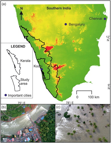
Kerala, characterized by all three physiographic divisions, namely highland (>75.0 m), midland (7.5–75.0 m) and coastal plain (<7.0 m), exhibits diverse geomorphic features, such as tall mountain peaks of Anaimudi (2695 m), 41 short-run west flowing rivers, and a coastal plain studded with several lagoon and barrier systems. For example, according to Joseph and Thrivikramji (2002) and Sajinkumar et al. (2017), several parts of the coastal plains (Vembanadkayal, Kuttanad, and the Kole lands of Thrissur) have their floor below the mean sea level. Many of the short-run rivers have multi-purpose water storage reservoirs and dams located in the highland and/or midland.

Sporadic events of intense rainfall (e.g., 177.5 mm on 17 August 2018, at Idukki) in the catchments of Western Ghats caused reservoirs to reach Full Reservoir Level (FRL) and resulting in the release of excess waters through flood gates (Duncombe 2018). The release of excess water, inundated parts of the Pathanamthitta, Alappuzha, Kottayam, Idukki, Ernakulam, Thrissur and Wayanad districts (Figure 1b,c). The floodwaters that resulted from the dam release inundated vast built-up areas and small towns in the downstream of the basins disrupting the life of hundreds of thousands of citizens, warranting relocation in safe shelters. Inundation in the Achankovil, Pamba, Manimala, Meenachal, Moovattupuzha, Periyar and Chalakudi river basins led to 445 deaths, uprooting of river shore trees, partial or complete destruction or water-logging of homes, shops, roads, and other civil infrastructure, and caused heavy siltation over the affected land.

Assessment of flood inundation is a pressing requirement as it forms a vital component to formulate plans and permits for future, assessing damages, estimating levels of compensations, and selecting appropriate land use and land planning in flood affected/prone areas (Moel et al. 2009, Ran and Nedovic-Budic 2016). Due to the availability of synoptic views and re-views, satellite remote sensing data are an excellent tool in disaster management. However, optically sensed satellite data will be of little use because visible and near-infrared sensor collected images over the Kerala region in SWM season have been concealed due to the persistent cloud cover (Eberhardt et al. 2016;). In addition, unlike for other natural hazards, data on the extent of flooding need to be captured before the water recedes or else, the classical-indirect-terrestrial signatures of flood need to be identified and enumerated. As documented by Henry et al. (2006), De Groeve (2010), and Greifeneder et al. (2014), cloud-penetrating, active radar sensors operating in the microwave region, may be used for flood inundation research, regardless of cloud coverage. Hence, a Sentinal-1A radar dataset was used in this research to map the floodwater covered area in Kerala during and following the August, 2018 flood event.

The use of Level 1, 20 m by 22 m spatial resolution, Sentinel-1A, C-band, Synthetic Aperture Radar (SAR) data for flood monitoring purposes are documented herein. Specifically, the 21 August 2018 scene, downloaded from the Alaska Satellite Facility (UAF 2018), was processed, and proved useful for flood inundation mapping. The data contain portions of the inundated districts of Alappuzha, Kottayam, Ernakulam, Idukki and Thrissur in Kerala, India.

Methodology

The methodology of Kussul et al. (2008), as outlined and recommended in the UN-SPIDER Knowledge Portal (http://www.un-spider.org/advisory-support/recommended-practices/recommended-practice-flood-mapping), was adopted for flood inundation mapping. Data processing was completed with the ESA SNAP 6.0 software program (ESA 2018a). A subset of data of study area, from Thrissur district in the north to Alleppey district in the south, was created for calibration. This subset was created by first undoing the default processor scaling, followed by reintroducing a new desired scaling. According to the Sentinel website (ESA 2018b), four (4) calibration look up tables are available for Level 1 products: beta, sigma, gamma or original Digital Number. A sigma calibration was performed for this study; this calibration procedure creates a new product with calibrated backscatter coefficients. The calibrated image was then filtered to remove noise using a speckle filtering process. The calibrated, noise removed, product was then subjected to binarisation by specifying a threshold value. In binarisation, the image is classified into a binary image of water and non-water pixels. Due to the specular nature of water against microwave signals, the water pixels have a very low backscatter coefficient and appear considerably darker. This threshold value is selected from the histogram of the data and a band math operation was carried out to extract all pixels below this value (Smith 1997; Horrit et al. 2003; Mason et al. 2007). The binary image (above threshold and below threshold) was imported to ArcGIS 10.4.1 and the area comprised of water pixels was computed.

Three Sentinel-2A optical images were downloaded from the USGS website (USGS 2018) for the pre-flood period (9 January 2018; 18 February 2018, and 21 February 2018). Sentinel-2A multi-spectral instrument (MSI) has 13 bands (from visible (VIS) to Short Wave Infrared (SWIR)) in various resolutions, namely VIS and near infrared (NIR) at 10 m; three vegetation red edge bands (2 SWIR bands and the narrow NIR band) at 20 m, and the water vapour, cirrus and coastal aerosol bands at 60 m, respectively (Du et al., 2016). The SWIR and VIS bands make this an excellent tool for mapping water bodies. Several algorithms exist for extracting water bodies from optical remote sensing data, including single band density slicing (Work and Gilmer 1976), unsupervised and supervised classification (Huang et al. 2014), and spectral water indices (Li et al. 2013). Among these methods, the spectral water index-based method is considered the most reliable, user-friendly, efficient and low in computational cost (Ryu et al. 2002).

The Sentinel-2A scenes were mosaicked and the water bodies were extracted by one such spectral water index called Modified Normalized Differential Water Index (MNDWI) (Xu 2006). The MNDWI was developed using Equation (1)(1) $${\mathit{\text{MNDWI}}}_{20m}=\frac{{\rho }_3^{20m}-{\rho }_{11}}{{\rho }_3^{20m}+{\rho }_{11}}$$(1) , by upscaling the 10 m green band to 20 m. (1) $${\mathit{\text{MNDWI}}}_{20m}=\frac{{\rho }_3^{20m}-{\rho }_{11}}{{\rho }_3^{20m}+{\rho }_{11}}$$(1)

In Equation (1)(1) $${\mathit{\text{MNDWI}}}_{20m}=\frac{{\rho }_3^{20m}-{\rho }_{11}}{{\rho }_3^{20m}+{\rho }_{11}}$$(1) , ${\rho }_{11}$ is the top of the atmosphere (TOA) reflectance of band 11 (SWIR) of Sentinel-2A and ${\rho }_3^{20m}$ is the TOA reflectance of the 20 m upscaled band 3 of the Sentinel-2A dataset. The value of ${\rho }_3^{20m}$ is calculated as the average value of the corresponding 2 × 2 ${\rho }_3$ values. The area of water bodies, in the area of interest (AOI) during the pre-flood, was extracted from this image and was compared with that of the flood period to estimate the percentage increase of water pixels and hence the extent of the flood water inundation.

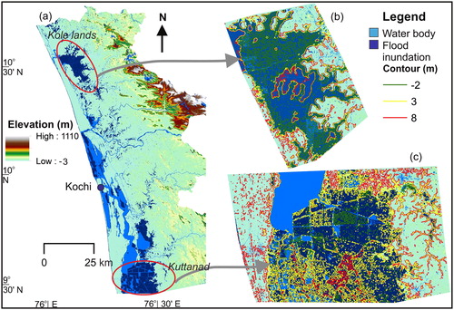
The Shuttle Radar Topographic Mission (SRTM) Digital Elevation Model (DEM) generated contour map was used to calculate the water level rise as a result of the flooding. The SRTM DEM, with a spatial resolution of 30 m, was obtained from the United States Geological Survey website (USGS 2018). The level of confidence (vertical accuracy) is ±16 m. A mosaic of the study area was prepared from three SRTM 1 arc second DEM tiles using ArcGIS 10.4.1. Contours for the Kuttanad and Kole Wetland regions were prepared from this DEM to visualize the water level due to recent floods.

Results and discussion

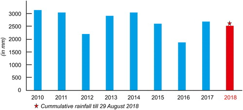
The state of Kerala experiences two monsoon seasons characterized by southwest (June to September) and northeast (October to December) monsoons. The spatio-temporal distribution of rainfall here is significantly influenced by the overall physiography of the state (Simon and Mohankumar 2004). Located in the western slopes of the Western Ghats, Kerala experiences heavy rainfall (roughly 3000 mm annually), of which, majority occur during the monsoon (Thomas and Prasannakumar 2016). The year 2018 experienced larger than normal rainfall with the southwest monsoon bringing an excess of 36% till the 29 August itself (Figure 2: Source IMD 2018) causing this deluge.

Figure 2. Hyetograph of Kerala from 2010 to 2018 (up to 29 August).

The extents of flood inundation in parts of south-central Kerala were effectively and reliably determined using processed Sentinel-1A data for 21 August 2018. Results show that the wetlands, consisting of low lying Kuttanad in the south, the Kole lands of Thrissur to the north, and the backwater system – Vembanad Kayal (Figure 3a), witnessed significant increase in water level and inundation due to the torrential rain generated catastrophic flood.

Figure 3. (a) Sentinel 2 image showing the water bodies of the study area before the flood event (b) Flood inundation map prepared from the water pixels of Sentinel 1 image of 21 August 2018 (c) Changes between the pre-event and the flood inundation map of the study area.

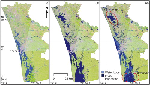
Though the flood waters in most of the inundated land in the river basins had already begun to recede by 21 August 2018, the water levels in the Kuttanad and Kole wetlands were slow to decline. As observed in Figure 3(b,c), the Kuttanad region in the south and the Kole wetlands in the north remained inundated in the 21 August, 2018, imagery. Furthermore, satellite image analysis showed a clear 89.6% increase in the area covered by water. The nearly twice as much area was covered with water when compared with any normal year is unequivocally a matter of grave concern.

Figure 4a is an overlay of DEM derived contours over the flood inundation vectors of Kuttanad and Kole wetlands. The rise in water levels in the Kole wetlands was up to ∼10 m (Figure 4b); while in the Kuttanad region it was up to ∼5 m (Figure 4c). Such a difference in the flood level is due to the geomorphology. Kuttanad is a vast basin with its floor lying below mean sea level, in contrast to physiographic highs surrounded Kole lands. This water level rise of 5–10 m is to be considered as a substantial rise and this rise is indicative of the disastrous and disruptive nature of the flood.

Figure 4. (a) DEM of the area showing pre-flood and flood, (b) flood inundation at Kole lands of Thrissur. Note the 10 m rise in water level during flooding and (c) flood inundation at Kuttanad. Note the 5 m rise in water level during flooding.

The typical geomorphic makeup and persistent water cover in the Kuttanad and Kole lands are the basis of the origin of a unique system of wetland agricultural practice prevailing in these areas. However, subsequent unscientific methods of land utilization, conversion of wetland to dry land, unbridled mining of river channel sand and brick clay, and construction of buildings for different end uses in the river floodplains, may have led to amplification of losses caused by the SWM rainfall events. This also caused a slowdown of free flow of flood waters through the ‘natural’ drainage system.

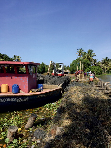
In Kuttanad, in addition to the extreme rainfall and opening of shutters of almost all the major dams, it was high tide time in the Arabian Sea and that further delayed the discharge of the flood waters. It was also observed by the authors in the field visit to Kuttanad that several bunds/embankments that secured the paddy polders and residential areas from the Vembanad Lake had experienced minor to major damages (Figure 5). These damages aggravated the flood effects as water from the Vembanad Lake started filling up the low lying paddy polders and residential areas.

Figure 5. View of the bund reconstruction efforts that secures Kanakassery, Valiyakari, and Meenapally paddy polders from the Vembanad Lake in Kuttanad. The left of the bund is the Vembanad Lake and the right of the bund is the paddy polders that span over 750 acres.

The National Disaster Response Force (NDRF) with the support of the Army and Navy carried out a major rescue effort evacuating over 10,000 people (Sabu and Joby 2018). However, these organized efforts by the government were not sufficient for rescue operations for a major flood of this magnitude. The volunteer efforts by the IEEE (Institute of Electrical and Electronics Engineers) Kerala Section to develop a crowd sourced tool to identify rescue and relief needs was valuable for timely action. The fishermen in the coastal districts of Kerala played an essential role in the rescue. They used their boats and resources to travel to the flood-affected areas and helped to save many lives.

The flood events of August 2018, in Kerala, should inaugurate the beginning of a new paradigm for redeveloping the affected area through a scheme of zoning based on the origin of landscape, extent, and depths of flood water levels at various geolocations vis-à-vis a better rainfall prediction. The floods of August 2018 maybe the new norm in the coming years and decades, especially in the backdrop of changing weather patterns globally.

Conclusions

The assessment of the 2018 August floods in Kerala using August 21 Sentinel-1A satellite imagery indicates that a 90% increase in water cover was observed due to the flooding. The measured water levels from satellite imagery and DEM for the region indicate that low lying areas in the coastal plains of Kuttanad and the Kole lands of Thrissur had a rise of water up to 5 m and 10 m, respectively. This study validates the findings of the previous studies (Prasad et al. 2006) on the applicability of multi-sensor satellite data in mapping flood hazards in India. The timely acquisition of the satellite data provides an opportunity to immediately identify the flooded regions for planning rescue and relief operations.

Combining the satellite-based approach with crowd sourced efforts to identify flooded locations and rescue needs can help better validate the crowd sourced approach and improve response for such extreme events in the future. It is evident from the rescue and relief efforts in Kerala that crowd sourcing and volunteered help is equally essential together with the government efforts using the military and para-military to save lives in extreme events of large magnitude.

Acknowledgements

Oommen and Coffman thankful to the National Science Foundation (NSF, USA) sponsored Geotechnical Extreme Events Reconnaissance (GEER) Association for underwriting the cost of travel to Kerala, India, to verify and document the flood footprint that is reported herein. Authors acknowledge the editor and the anonymous reviewer for constructive comments.

Disclosure statement

No potential conflict of interest was reported by the author(s).

References

- De Groeve T. 2010. Flood monitoring and mapping using passive microwave remote sensing in Namibia. Geomat, Nat Haz Risk. 1(1):19–35.
- De US, Dube RK, Rao GP. 2005. Extreme weather events over India in the last 100 years. J Ind Geophys Union. 9(3):173–187.
- Duncombe J. 2018. Making sense of landslide danger after Kerala’s floods. Eos. 99. https://doi.org/10.1029/2018EO108061.
- Du Y, Zhang Y, Ling F, Wang Q, Li W, Li X. 2016. Water bodies’ mapping from Sentinel-2 imagery with Modified Normalized Difference Water Index at 10-m spatial resolution produced by sharpening the SWIR Band. Remote Sensing. 8(4):354.
- Eberhardt I, Schultz B, Rizzi R, Sanches I, Formaggio A, Atzberger C, Mello M, Immitzer M, Trabaquini K, Foschiera W, José Barreto Luiz A. 2016. Cloud cover assessment for operational crop monitoring systems in tropical areas. Remote Sens. 8(3):219.
- ESA 2018a. http://step.esa.int
- ESA 2018b. http://sentinel.esa.int
- Greifeneder F, Wagner W, Sabel D, Naeimi V. 2014. Suitability of SAR imagery for automatic flood mapping in the Lower Mekong basin. Int J Remote Sens. 35(8):2857–2874.
- Gupta K. 2007. Urban flood resilience planning and management and lessons for the future: a case study of Mumbai, India. Urban Water J. 4(3):183–194.
- Henry JB, Chastanet P, Fellah K, Desnos YL. 2006. Envisat multi‐polarized ASAR data for flood mapping. Int J Remote Sens. 27(10):1921–1929.
- Huang C, Chen Y, Wu J. 2014. Mapping spatio-temporal flood inundation dynamics at large river basin scale using time-series flow data and MODIS imagery. Int J Appl Earth Observ Geoinf. 26350–362.
- IMD 2018. India Meteorological Department. www.imd.gov.in
- Joseph S, Thrivikramji KP. 2002. Kayals of Kerala Coastal Land and Implication to Quaternary Sealevel Changes. Memo Geol Soc Ind. 4951–64.
- Kussul N, Shelestov A, Skakun S. 2008. Grid system for flood extent extraction from satellite images. Earth Sci Inform. 1(3–4):105.
- Li W, Du Z, Ling F, Zhou D, Wang H, Gui Y, Sun B, Zhang X. 2013. A comparison of land surface water mapping using the normalized difference water index from TM, ETM + and ALI. Remote Sens. 5(11):5530–5549.
- Mason DC, Horritt MS, Dall'Amico JT, Scott TR, Bates PD. 2007. Improving river flood extent delineation from synthetic aperture radar using airborne laser altimetry. IEEE Trans Geosci Remote Sens. 45(12):3932–3943.
- Moel HD, van Alphen J, Aerts JCJH. 2009. Flood maps in Europe-methods, availability and use. Nat Hazards Earth Syst Sci. 9(2):289–301.
- Prasad AK, Kumar KK, Singh S, Singh RP. 2006. Potentiality of multi-sensor satellite data in mapping flood hazard. J Indian Soc Remote Sens. 34(3):219–331.
- Ran J, Nedovic-Budic Z. 2016. Integrating spatial planning and flood risk management: A new conceptual framework for the spatially integrated policy infrastructure. Comput, Environ Urban Syst. 57:68–79.
- Rao KHVD, Rao VV, Dadhwal VK, Diwakar PG. 2014. Kedarnath flash floods: a hydrological and hydraulic simulation study. Curr Sci. 106(4):598–603.
- Ryu JH., Won JS, Min KD. 2002. Waterline extraction from landsat TM data in a tidal flat—A case study in Gomso Bay, Korea. Remote Sens. Environ. 83, 442–456.
- Sabu S, Joby NE. 2018. Kerala floods-Rescue and rehabilitation using information technology and social media. https://blogs.agu.org/thefield/2018/09/21/kerala-floods-rescue-and-rehabilitation-using-information-technology-and-social-media/
- Sajinkumar KS, Kannan JP, Indu GK, Muraleedharan C, Rani VR. 2017. A composite fall-slippage model for cliff recession in the sedimentary coastal cliffs. Geosci Front. 8(4):903–914.
- Sarkar S, Singh RP. 2017. June 19 2015 rainfall event over Mumbai: Some observational analysis. J Indian Soc Remote Sens. 45(1):185–192.
- Sati SP, Gahalaut VK. 2013. The fury of the floods in the north-west Himalayan region: the Kedarnath tragedy. Geom, Nat Haz Risk. 4(3):193–201.
- Simon A, Mohankumar K. 2004. Spatial variability and rainfall characteristics of Kerala. J Earth Syst Sci. 113(2):211–221.
- Smith LC. 1997. Satellite remote sensing of river inundation area, stage, and discharge: a review. Hydrol Process. 11(10):1427–1439.
- Thomas J, Prasannakumar V. 2016. Temporal analysis of rainfall (1871–2012) and drought characteristics over a tropical monsoon-dominated state (Kerala) of India. J Hydrol. 534266–280.
- UAF 2018. https://vertex.daac.asf.alaska.edu/
- USGS 2018. https://earthexplorer.usgs.gov/
- Work EA, Jr, Gilmer DS. 1976. Utilization of satellite data for inventorying prairie ponds and lakes. Ann Arbor. 100148107.
- Xu H. 2006. Modification of normalised difference water index (NDWI) to enhance open water features in remotely sensed imagery. Int J Remote Sens. 27(14):3025–3033.