Solution for a time-series AR model based on robust TLS estimation

Abstract

We discuss an algorithm for the autoregression (AR) model as a typical time-series model. By analyzing the structure of the AR model, we highlight the shortcomings of traditional algorithms for model parameter estimation and propose an approach to overcome the shortcomings of traditional solutions for the AR model. The errors-in-variables (EIV) model is used to solve an existing problem. There is an obvious difference between the AR model and a traditional model. For the AR model, one observation datum appears repeatedly; hence, the residual of one observation datum is not unique. Furthermore, in theory, the optimal estimation of model parameters cannot be obtained by current solutions. Based on an analysis of the AR model, we focus on how to obtain the optimal estimation when the observation data of the AR model are contaminated by outliers. The median function is used to establish a modified solution for the AR model based on the institute of geodesy & geophysics, Chinese academy of sciences (IGG) weight function by comparison with current algorithms for the robust estimation of the EIV model. We propose an iterative algorithm based on median function. Finally, we apply two numerical instances to compare the proposed algorithm with traditional algorithms and draw conclusions from results of the instances.

Keywords:

• Autoregression model
• errors-in-variables
• robust estimation
• median function

1. Introduction

The time-series model is widely used in the relative fields of prediction, such as solar irradiance prediction, ground subsidence prediction and weather prediction (Zhangzhen and Tianhe 2012; Hirata and Aihara 2017; do Nascimento Camelo et al. 2018; Tuncel and Baydogan 2018). The autoregression (AR) model is a typical time-series model, and the theory based on AR model is developed. Time dimensions are taken into account when the variables described by AR model are related to time (Pfeifer and Deutsch 1980; Pfeifer and Ve Bodily 1990); when stochastic character of AR model has an influence on estimation model parameters, this factor is also investigated (Di Giacinto 2006); besides, AR model with Kalman filter is proposed for non-linear estimators (Kurt and Batu Tunay 2015). As a mathematical fitting model, the precision of the AR model’s parameter estimation determines the efficiency of a prediction (Wan and Xiao 2016; Datteo et al. 2018). Currently, traditional algorithms for parameter estimation for the AR model involve transforming the AR model into the Gauss–Markov model (G–M model) and computing the model parameters based on least-squares (LS) estimation. The computation process is expressed as follows: $$\{\begin{array}{c}\mathit{v}=\mathit{Bx}-\mathit{l}\\ \mathit{v}\sim N(0,{\sigma }_0^2{\mathit{P}}^{-1})\\ {\mathit{v}}^T\mathit{Pv}=min\end{array}\to \{\begin{array}{c}\widehat{\mathit{x}}={\left({\mathit{B}}^T\mathit{PB}\right)}^{-1}{\mathit{B}}^T\mathit{Pl}\\ {\widehat{\sigma }}_0^2=\frac{{\mathit{v}}^T\mathit{Pv}}{r}\\ \mathit{D}\left(\widehat{\mathit{x}}\right)\approx {\widehat{\sigma }}_0^2{\left({\mathit{B}}^T\mathit{PB}\right)}^{-1}\end{array}$$

where v is the error vector that exists in the observation vector (l), which is composed of observation data; v follows a normal distribution. B is the coefficient matrix that expresses the relationship between the observation vector (l) and model parameters vector (x). In a stochastic model, ${\sigma }_0^2$ is the variance component of the unit weight, and its estimation is written as ${\widehat{\sigma }}_0^2$. P is the weight matrix. Based on LS(v^TPv = min), the model parameters (x) can be estimated, and the estimation is written as $\widehat{\mathit{x}}$. D($\widehat{\mathit{x}}$) denotes the covariance matrix, whereas r denotes redundancy.

A traditional solution for model parameter estimation only takes into account the observation error in the observation vector by implementing least constraints on it; however, as highlighted by Adcock (1877), the shortcomings of a traditional solution are that it ignores the error that exists in the coefficient matrix, and the elements of the coefficient matrix are also composed of observation data. To take into account errors that exist in the observation vector and coefficient matrix simultaneously, the G–M model was developed, and a more scientific model called the errors-in-variables model (EIV model; Adcock 1877) was proposed and written as follows: (1) $$\{\begin{array}{c}\mathit{v}=(\mathit{B}+{\mathit{E}}_B)\mathit{x}-\mathit{l}\\ \left[\begin{array}{c}\mathit{v}\\ \mathit{b}\end{array}\right]\sim N\left(\left[\begin{array}{c}0\\ 0\end{array}\right],{\sigma }_0^2\left[\begin{array}{cc}{\mathit{P}}^{-1}& 0\\ 0& {\mathit{P}}_B^{-1}\end{array}\right]\right)\end{array}$$(1)

where E_B is the error matrix that exists in the coefficient matrix (B), b = vec(E_B)(vec(·) represents the vector that stacks one column of E_B underneath the previous one, and P_B denotes the weight matrix of the coefficient matrix. To take into account both observation errors in the observation vector and coefficient matrix, total least squares (TLS) is proposed to extend the traditional criterion of LS: (2) $${\mathit{v}}^T\mathit{Pv}+{\mathit{b}}^T{\mathit{P}}_B\mathit{b}=min$$(2)

Researchers have discussed optimal solutions for the EIV model (Golub and Van Loan 1980; Schaffrin and Wieser 2008; Mahboub 2014; Ai-Sharadqah and Ho 2018), and it is extensively used in relative fields of geoscience (Schaffrin and Uzun 2011; Mahboub 2012; Wang et al. 2016; Leyang et al. 2017).

In this article, we introduce the EIV model into time-series prediction, in addition to discussing a solution for AR model parameter estimation based on TLS. Particularly, the optimal algorithm for robust estimation is discussed when the observation data in the AR model are contaminated by outliers. This remainder of this article is organized as follows: in Section 2, the AR model is shown in the form of the EIV model, and the difference between the AR model and traditional EIV model is analyzed. In Section 3, traditional solutions for AR model parameter estimation are presented first. Then, a modified solution for AR model parameter estimation while outliers exist in the observation data is proposed, where the proposed solution is based on robust estimation and the median function. In Section 4, the feasibility and efficiency of the proposed solution are proved using two numerical instances.

2. AR model and traditional solutions for robust estimation

2.1. EIV model and its solution

Suppose that the quantity of model parameters is m, such that $(a_1,a_2,\dots ,a_m)$, and the quantity of observation data is m + n, such that $(h_1,h_2,\dots ,h_{m+n})$. Then, the AR model can be expressed as follows: (3) $$\{\begin{array}{c}{h}_{m+1}=a_1{h}_1+a_2{h}_2+\cdots +a_m{h}_m\\ h_{m+2}=a_1{h}_2+a_2{h}_3+\cdots +a_m{h}_{m+1}\\ ⋮\\ h_{m+n}=a_1{h}_n+a_2{h}_{n+1}+\cdots +a_m{h}_{m+n-1}\end{array}$$(3)

The AR model can be rewritten using the G–M model as follows: (4) $$\underset{\mathit{v}}{\underbrace{\left[\begin{array}{c}{v}_{m+1}\\ v_{m+2}\\ ⋮\\ v_{m+n}\end{array}\right]}}+\underset{\mathit{l}}{\underbrace{\left[\begin{array}{c}{h}_{m+1}\\ h_{m+2}\\ ⋮\\ h_{m+n}\end{array}\right]}}=\underset{\mathit{B}}{\underbrace{\left[\begin{array}{cccc}{h}_1& h_2& \cdots & h_m\\ h_2& h_3& \cdots & h_{m+1}\\ ⋮& ⋮& ⋮& ⋮\\ h_n& h_{n+1}& \cdots & h_{m+n-1}\end{array}\right]}}\underset{\mathit{x}}{\underbrace{\left[\begin{array}{c}{a}_1\\ a_2\\ ⋮\\ a_m\end{array}\right]}}$$(4)

where $(v_{m+1},v_{m+2},\dots ,v_{m+n})$ is an error vector that exists in the observation vector (l), which is denoted as v in the equation. If we transpose the observation vector from the left-hand side to the right-hand side of Equation (4)(4) $$\underset{\mathit{v}}{\underbrace{\left[\begin{array}{c}{v}_{m+1}\\ v_{m+2}\\ ⋮\\ v_{m+n}\end{array}\right]}}+\underset{\mathit{l}}{\underbrace{\left[\begin{array}{c}{h}_{m+1}\\ h_{m+2}\\ ⋮\\ h_{m+n}\end{array}\right]}}=\underset{\mathit{B}}{\underbrace{\left[\begin{array}{cccc}{h}_1& h_2& \cdots & h_m\\ h_2& h_3& \cdots & h_{m+1}\\ ⋮& ⋮& ⋮& ⋮\\ h_n& h_{n+1}& \cdots & h_{m+n-1}\end{array}\right]}}\underset{\mathit{x}}{\underbrace{\left[\begin{array}{c}{a}_1\\ a_2\\ ⋮\\ a_m\end{array}\right]}}$$(4) , then the standard expression of the G–M model can be obtained as v = Bx - l, and the model parameters can be obtained using the method presented in the previous section. Note that elements of the coefficient matrix also consist of observation data; hence, there are observation errors in the coefficient matrix. If we define E_B as the error matrix that exists in the coefficient matrix, then Equation (4)(4) $$\underset{\mathit{v}}{\underbrace{\left[\begin{array}{c}{v}_{m+1}\\ v_{m+2}\\ ⋮\\ v_{m+n}\end{array}\right]}}+\underset{\mathit{l}}{\underbrace{\left[\begin{array}{c}{h}_{m+1}\\ h_{m+2}\\ ⋮\\ h_{m+n}\end{array}\right]}}=\underset{\mathit{B}}{\underbrace{\left[\begin{array}{cccc}{h}_1& h_2& \cdots & h_m\\ h_2& h_3& \cdots & h_{m+1}\\ ⋮& ⋮& ⋮& ⋮\\ h_n& h_{n+1}& \cdots & h_{m+n-1}\end{array}\right]}}\underset{\mathit{x}}{\underbrace{\left[\begin{array}{c}{a}_1\\ a_2\\ ⋮\\ a_m\end{array}\right]}}$$(4) can be rewritten using the EIV model as v = (B + E_B)x - l. To obtain the optimal estimation of the EIV model parameters, the criterion of TLS is defined as Equation (2)(2) $${\mathit{v}}^T\mathit{Pv}+{\mathit{b}}^T{\mathit{P}}_B\mathit{b}=min$$(2) . Many solutions have been established for the EIV model, as cited previously. Typical solutions that can take into account the stochastic character of the model were proposed (Schaffrin and Wieser 2008; Mahboub 2014; Fang et al. 2017). In this article, we choose the iterative solution proposed by Schaffrin and Wieser (2008) as an example: (5) $$\{\begin{array}{c}\widehat{\mathit{x}}=({\mathit{B}}^T{(\mathit{Q}+{(({\widehat{\mathit{x}}}^T{\mathit{Q}}_0\widehat{\mathit{x}}){\mathit{Q}}_{\mathit{b}})}^{-1}\mathit{B}-\widehat{\mathit{\delta }}{\mathit{Q}}_0)}^{-1}{\mathit{B}}^T{(\mathit{Q}+({\widehat{\mathit{x}}}^T{\mathit{Q}}_0\widehat{\mathit{x}}){\mathit{Q}}_{\mathit{b}})}^{-1}\mathit{l}\\ \widehat{\mathit{v}}=-\mathit{Q}\widehat{\mathit{\lambda }}\\ {\widehat{\mathit{E}}}_{\mathit{B}}={\mathit{Q}}_{\mathit{b}}\widehat{\mathit{\lambda }}{\widehat{\mathit{x}}}^T{\mathit{Q}}_0\end{array}$$(5)

where $\widehat{\mathit{x}}$, $\widehat{\mathit{v}}$ and ${\widehat{\mathit{E}}}_{\mathit{B}}$ are estimations of the relative parameters; Q, Q₀ and Q_b are cofactor matrices; and $\mathit{P}={\mathit{Q}}_{}^{-1}$ and ${\mathit{P}}_B={\mathit{Q}}_0^{-1}\otimes {\mathit{Q}}_b^{-1}$, where $\otimes$ represents the symbol of the Kronecker–Zehfuss product. $\widehat{\lambda }$ is the estimation of Lagrange multipliers $\mathit{\lambda }$, $\widehat{\mathit{\delta }}={\widehat{\mathit{\lambda }}}^T{\mathit{Q}}_b\widehat{\mathit{\lambda }}$. The detailed iteration can be found in the seminal report of Schaffrin and Wieser (2008).

Additionally, by Equation (4)(4) $$\underset{\mathit{v}}{\underbrace{\left[\begin{array}{c}{v}_{m+1}\\ v_{m+2}\\ ⋮\\ v_{m+n}\end{array}\right]}}+\underset{\mathit{l}}{\underbrace{\left[\begin{array}{c}{h}_{m+1}\\ h_{m+2}\\ ⋮\\ h_{m+n}\end{array}\right]}}=\underset{\mathit{B}}{\underbrace{\left[\begin{array}{cccc}{h}_1& h_2& \cdots & h_m\\ h_2& h_3& \cdots & h_{m+1}\\ ⋮& ⋮& ⋮& ⋮\\ h_n& h_{n+1}& \cdots & h_{m+n-1}\end{array}\right]}}\underset{\mathit{x}}{\underbrace{\left[\begin{array}{c}{a}_1\\ a_2\\ ⋮\\ a_m\end{array}\right]}}$$(4) , an obvious characteristic of the AR model can be determined such that the same element appears in the model repeatedly: the quantity of one element in vector ($\begin{array}{cccc}{h}_1,& h_2,& \cdots ,& h_m\end{array}$) that appears in the AR model is (1, 2, …, m), respectively, whereas ($\begin{array}{cccc}{h}_{m+1},& h_{m+2},& \cdots ,& h_{m+n}\end{array}$) is (n, …,1), respectively. Thus, although the AR model belongs to the catalogue of EIV models, solutions for the traditional EIV model may not be suitable for the AR model because, in a mathematical model, one observation datum should obtain a unique residual or the same residual; however, current solutions cannot ensure that the observation datum meets this requirement, which results from the condition that one observation datum appears in the model repeatedly. Furthermore, this fact has an influence on the optimal algorithm, particularly for robust estimation, which is the main problem addressed in the following discussion.

2.2. Analysis of traditional robust estimation for the AR model

According to the previous analysis, to take into account the observation error in the observation vector and coefficient matrix, the EIV model is considered to be a rational solution for the parameter estimation of the AR model. However, the factor that one observation datum obtains different residuals because of its repeated appearance cannot be overcome by current solutions. Such a phenomenon has an influence on, for example, parameter estimation and precision statistics, particularly for robust estimation. In fact, the observation data are contaminated by an observation error unavoidably. When the error belongs to the stochastic error, criteria such as LS and maximum likelihood estimation are used to obtain the optimal estimation of model parameters. In the intervening time, when the observation data are contaminated by outliers, robust estimation is used to overcome the influence that outliers have on parameter estimation. As is well known, to overcome the influence of outliers that exist in the observation data, the method of robust estimation uses a weight function, such as the Huber weight function (Huber 1964) and IGG weight function (Yang 1999), to modify the weight of the observation data. Considering the IGG weight function, for example, (6) $${\overline{P}}_i=\{\begin{array}{c}{P}_i,\hspace{1em}\hspace{1em}\left|{\widehat{v}}_i\right|\le a\\ P_{i}a/\left|{\widehat{v}}_i\right|,\hspace{1em}\hspace{1em}a<\left|{\widehat{v}}_i\right|\le b\\ 0,b<\left|{\widehat{v}}_i\right|\end{array}$$(6)

where P_i is the initial weight value of the observation data; $\left|{\widehat{v}}_i\right|$ is the absolute value of the residual for the observation data; a and b denote the threshold value; and their values are often $a=1.5\hspace{0.17em}\sigma$ and $b=2.5\hspace{0.17em}\sigma$, where$\sigma$ is a variance component.

Robust estimation uses the weight function to modify the weight value of the observation data. Generally, poorly accurate observation data that are assessed by the residual obtain a smaller weight value, and its influence on parameter estimation can be modified properly. In this process, observation data precision is assessed by the residual. The IGG weight function has three segments:

1. If the residual is smaller than or equal to threshold value a, then the weight of observation data remains invariant.

2. If the residual is greater than threshold value a but smaller than or equal to threshold value b, then the weight of the observation data should be modified and becomes smaller according to the formula.

3. If the residual is greater than threshold value b, then zero is assigned to the weight of the observation data.

For the EIV model, the residuals of the observation vector and coefficient matrix are obtained by current solutions; however, as shown in the previous analysis, solutions for the AR model based on TLS make one observation datum obtain different residuals, which could lead to failure in the utilization weight function for robust estimation.

3. Iterative algorithm for the AR model

According to the analysis in the previous section, the AR model is different from the traditional EIV model. The obvious characteristic is that one observation datum appears in the model repeatedly. This phenomenon causes the observation datum to obtain different residuals. As cited in Equation (4)(4) $$\underset{\mathit{v}}{\underbrace{\left[\begin{array}{c}{v}_{m+1}\\ v_{m+2}\\ ⋮\\ v_{m+n}\end{array}\right]}}+\underset{\mathit{l}}{\underbrace{\left[\begin{array}{c}{h}_{m+1}\\ h_{m+2}\\ ⋮\\ h_{m+n}\end{array}\right]}}=\underset{\mathit{B}}{\underbrace{\left[\begin{array}{cccc}{h}_1& h_2& \cdots & h_m\\ h_2& h_3& \cdots & h_{m+1}\\ ⋮& ⋮& ⋮& ⋮\\ h_n& h_{n+1}& \cdots & h_{m+n-1}\end{array}\right]}}\underset{\mathit{x}}{\underbrace{\left[\begin{array}{c}{a}_1\\ a_2\\ ⋮\\ a_m\end{array}\right]}}$$(4) , one element in vector ($\begin{array}{cccc}{h}_1,& h_2,& \cdots ,& h_m\end{array}$) appears in the equation (1(1) $$\{\begin{array}{c}\mathit{v}=(\mathit{B}+{\mathit{E}}_B)\mathit{x}-\mathit{l}\\ \left[\begin{array}{c}\mathit{v}\\ \mathit{b}\end{array}\right]\sim N\left(\left[\begin{array}{c}0\\ 0\end{array}\right],{\sigma }_0^2\left[\begin{array}{cc}{\mathit{P}}^{-1}& 0\\ 0& {\mathit{P}}_B^{-1}\end{array}\right]\right)\end{array}$$(1) , 2, …, m) times, respectively, whereas (h_m+1, h_m+2, …, h_m+n) is (n, …,1), respectively. Therefore, if we define ${\mathit{\Delta }}_i$(i = 1, 2, …, m + n), which represents the observation error in the observation data, then the observation error that exists in the observation vector (h₁, …, h_m, h_m+1,…, h_m+n) can be expressed as (${\mathit{\Delta }}_1,\dots ,{\mathit{\Delta }}_m,{\mathit{\Delta }}_{m+1},\dots ,{\mathit{\Delta }}_{m+n}$), and the elements of error vector ${\mathit{\Delta }}_i$ are as follows: (7) $$\{\begin{array}{c}{\mathit{\Delta }}_1=[{\Delta }_1]\\ ⋮\\ {\mathit{\Delta }}_m=[\begin{array}{ccc}{\Delta }_m^1& \cdots & {\Delta }_m^m\end{array}]\\ \begin{array}{c}{\mathit{\Delta }}_{m+1}=[\begin{array}{ccc}{\Delta }_{m+1}^1& \cdots & {\Delta }_{m+1}^n\end{array}]\\ \begin{array}{c}⋮\\ {\mathit{\Delta }}_{m+n}=[{\Delta }_{m+n}]\end{array}\end{array}\end{array}$$(7)

To obtain a unique residual for the observation data, we use the median function (med[•]): (8) $$\{\begin{array}{c}{v}_1=\sqrt{\text{med}\left[{\left({\Delta }_1\right)}^2\right]}\\ ⋮\\ v_m=\sqrt{\text{med}\left[\begin{array}{ccc}{\left({\Delta }_m^1\right)}^2& \cdots & {\left({\Delta }_m^m\right)}^2\end{array}\right]}\\ \begin{array}{c}{v}_{m+1}=\sqrt{\text{med}\left[\begin{array}{ccc}{\left({\Delta }_{m+1}^1\right)}^2& \cdots & {\left({\Delta }_{m+1}^n\right)}^2\end{array}\right]}\\ \begin{array}{c}⋮\\ v_{m+n}=\sqrt{\text{med}\left[{\left({\Delta }_{m+n}\right)}^2\right]}\end{array}\end{array}\end{array}$$(8)

The unique observation error of the observation data can be obtained using the median function. Additionally, the median function is robustly efficient; in seminal reports (Rousseeuw and Wagner 1994), conclusions have indicated that when the contamination rate of outliers that exist in the observation data is not more than 50%, solutions based on the median function can obtain a stable estimation for model parameters. Furthermore, we use the median function to obtain the variance component, which is a vital parameter for the weight function and robust estimation: (9) $$\sigma =1.483•\text{med}[v_1,v_2,\cdots ,v_{m+n}]$$(9)

whereas the variance component is typically computed as follows: (10) $$\sigma =\sqrt{[v_1{v}_2\cdots v_{m+n}]{\mathit{P}}_{m+n}{[v_1{v}_2\cdots v_{m+n}]}^T/r}$$(10)

where P_m+n is the weight matrix of the observation data. Note that the estimation of the variance component is biased by the current solutions (Shen et al. 2011). The efficiency of above two methods for computing the variance component will be compared by instance in the next section.

An iterative algorithm for robust TLS estimation is established for the AR model using the median function:

Step 1. Calculate the initial values of the AR model parameters using algorithms based on the TLS criteria: $${\widehat{\mathit{x}}}^0=({\mathit{B}}^T{(\mathit{Q}+{(({\widehat{\mathit{x}}}^T{\mathit{Q}}_0\widehat{\mathit{x}}){\mathit{Q}}_{\mathit{b}})}^{-1}\mathit{B}-\widehat{\delta }{\mathit{Q}}_0)}^{-1}{\mathit{B}}^T{(\mathit{Q}+({\widehat{\mathit{x}}}^T{\mathit{Q}}_0\widehat{\mathit{x}}){\mathit{Q}}_{\mathit{b}})}^{-1}\mathit{l}$$

Step 2. Calculate the residuals of the observation data in the coefficient matrix and observation vector, respectively: $$\{\begin{array}{c}\widehat{\mathit{v}}=-\mathit{Q}\widehat{\mathit{\lambda }}\\ {\widehat{\mathit{E}}}_{\mathit{B}}={\mathit{Q}}_{\mathit{b}}\widehat{\mathit{\lambda }}{\widehat{\mathit{x}}}^T{\mathit{Q}}_0\end{array}$$

Step 3. Calculate the unique residual of each observation datum based on Equations (7)(7) $$\{\begin{array}{c}{\mathit{\Delta }}_1=[{\Delta }_1]\\ ⋮\\ {\mathit{\Delta }}_m=[\begin{array}{ccc}{\Delta }_m^1& \cdots & {\Delta }_m^m\end{array}]\\ \begin{array}{c}{\mathit{\Delta }}_{m+1}=[\begin{array}{ccc}{\Delta }_{m+1}^1& \cdots & {\Delta }_{m+1}^n\end{array}]\\ \begin{array}{c}⋮\\ {\mathit{\Delta }}_{m+n}=[{\Delta }_{m+n}]\end{array}\end{array}\end{array}$$(7) and (8)(8) $$\{\begin{array}{c}{v}_1=\sqrt{\text{med}\left[{\left({\Delta }_1\right)}^2\right]}\\ ⋮\\ v_m=\sqrt{\text{med}\left[\begin{array}{ccc}{\left({\Delta }_m^1\right)}^2& \cdots & {\left({\Delta }_m^m\right)}^2\end{array}\right]}\\ \begin{array}{c}{v}_{m+1}=\sqrt{\text{med}\left[\begin{array}{ccc}{\left({\Delta }_{m+1}^1\right)}^2& \cdots & {\left({\Delta }_{m+1}^n\right)}^2\end{array}\right]}\\ \begin{array}{c}⋮\\ v_{m+n}=\sqrt{\text{med}\left[{\left({\Delta }_{m+n}\right)}^2\right]}\end{array}\end{array}\end{array}$$(8) , which was proposed previously. The unique residuals of all observation data are listed as (v₁, v₂, …, v_m+n).

Step 4. Calculate the variance component ($\widehat{\sigma }$) using Equation (9)(9) $$\sigma =1.483•\text{med}[v_1,v_2,\cdots ,v_{m+n}]$$(9) and redefine the weight based on the weight function. The IGG weight function is used in this article: $${\overline{P}}_i=\{\begin{array}{c}{P}_i,\left|{\widehat{v}}_i\right|\le a\\ P_{i}a/\left|{\widehat{v}}_i\right|,\hspace{1em}a<\left|{\widehat{v}}_i\right|\le b\\ 0,b<\left|{\widehat{v}}_i\right|\end{array}$$

Note that the threshold value and residual estimation (${\widehat{v}}_i$) of the weight function should be calculated based on $\widehat{\sigma }$ and (v₁, v₂, …, v_m+n), which were proposed previously.

Step 5. Calculate the model parameters and iteration from Step 2 to Step 4 until the estimation converges.

This algorithm is called robust M-TLS in this article.

4. Numerical examples and discussion

In this section, two numerical examples are used to verify the proposed robust TLS estimation for the AR model. The aims of these examples are as follows:

(I) The first instance uses real observation data, and we compare the differences of solutions for the AR model between LS and TLS. The model for which both the coefficient matrix and observation vector have observation errors is computed using LS and TLS, respectively. The results based on the two solutions are compared with each other.

(II) The second example uses simulated data, and we insert simulated outliers into the EIV model. The traditional algorithm for robust LS is used to calculate the model parameters. Meanwhile, both the robust TLS algorithm and robust M-TLS algorithm are also used to calculate the model parameters. The results are compared with each other to verify the efficiency of the different algorithms.

In the instances, three parameters are used for the AR model, which can be written as follows: $$\{\begin{array}{c}{h}_4=a_1{h}_1+a_2{h}_2+a_3{h}_3\\ h_5=a_1{h}_2+a_2{h}_3+a_3{h}_4\\ ⋮\\ h_{m+n}=a_1{h}_{m+n-3}+a_2{h}_{m+n-2}+a_3{h}_{m+n-1}\end{array}$$

Observation data of first instance are listed in Table 1. Before proceeding to the experiment, stationary of observation data has been analyzed, autocorrelation function of the observation data is calculated and it is presented in Figure 1.

Figure 1. Autocorrelation analysis of observation data.

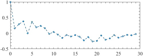
Table 1. Observation data of first instance/mm.

Dot mark	Observation data	Dot mark	Observation data	Dot mark	Observation data
1	15.054	11	14.839	21	17.389
2	14.986	12	16.003	22	15.467
3	15.159	13	15.394	23	15.962
4	14.271	14	16.675	24	16.734
5	15.539	15	15.456	25	15.535
6	15.278	16	16.254	26	17.215
7	14.655	17	14.033	27	16.400
8	15.156	18	15.613	28	15.294
9	15.234	19	16.802	29	17.088
10	14.180	20	15.500	30	16.669

Using real observation data that are supposed to only have a random error, model parameters are calculated using TLS and LS, respectively. The results are listed in Table 2, including the accuracy indices of the unit weight of variance component (${\sigma }_0$) and mean absolute per cent error (MAPE), which is calculated using the observation data of No. 1–No. 20 and check data of No. 21–No. 30, respectively. The results demonstrate that for the EIV model, the TLS algorithm has an advantage over the LS algorithm.

Table 2. Results of model parameters calculated using two algorithms.

	a1	a2	a3	${\sigma }_0$	MAPE
LS	0.408267	0.365555	0.233154	0.8810	6.03
TLS	0.552274	0.316370	0.139416	0.7951	4.88

In the second example, values of (a₁, a₂, a₃) are simulated as (0.6, −0.4, −0.2), and the observation data calculated using the simulated parameters are listed in Table 3. The previous 25 periods’ observation data are used to calculate the model parameters, and other observation data are used to check the precision of the parameters. To achieve the aforementioned aims, a random error that follows N(0, 1) is inserted into the previous 25 periods’ observation data, which is shown in Figure 2.

Figure 2. Distribution of a random error inserted into the observation data.

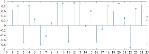
Table 3. Observation data of the AR model/m.

Dot mark	Observation data	Dot mark	Observation data	Dot mark	Observation data
1	15. 918	13	−0. 239	25	4. 733
2	14. 797	14	−7. 783	26	−5. 544
3	23. 246	15	7. 000	27	0. 221
4	−1. 017	16	1. 569	28	5. 013
5	−0. 217	17	−7. 784	29	−4. 417
6	14. 398	18	5. 129	30	−0. 989
7	−3. 403	19	3. 029	31	4. 973
8	−5. 209	20	−7. 328	32	−3. 249
9	11. 042	21	3. 331	33	−1. 933
10	−2. 167	22	4. 082	34	4. 670
11	−7. 108	23	−6. 546	35	−2. 110
12	8. 913	24	1. 675	36	−2. 605

The observation data of No. 1–No. 25 which are used to calculate model parameters are inserted into the random error, and their values are listed in Table 4. Additionally, outliers are inserted into the observation data of No. 4, No. 10, No. 18, and No. 25, which are denoted in red in Table 4.

Table 4. Observation data that are inserted into the random error/m.

Dot mark	Observation data	Dot mark	Observation data	Dot mark	Observation data
1	16. 547	10	−1. 237/1.237	19	3. 613
2	15. 609	11	−7. 793	20	−6. 409
3	22. 500	12	9. 854	21	3. 642
4	−0. 190/−2.190	13	0. 675	22	3. 153
5	0. 048	14	−7. 812	23	−5. 848
6	13. 593	15	7. 601	24	2. 543
7	−3. 846	16	0. 853	25	5. 090/7.090
8	−5. 115	17	−7. 940
9	11. 957	18	5. 960/3.960

Observation data in red denote that the data are contaminated by outliers.

Four observation data are inserted into outliers. Note that, for the AR model, if LS is used to calculate the model parameters, then the contamination rate of outliers is 4/22 (approximately 18.2%). Additionally, if TLS is used to calculate the model parameters, then the contamination rate of the outliers is 13/88 (approximately 14.8%). It appears that, for the AR model, when the same observation data are contaminated by outliers, the contamination rate based on TLS is smaller than that for LS.

When the observation data are contaminated by outliers, then we use three types of robust algorithms, that is robust LS, robust TLS and robust M-TLS proposed in this article to compute the model parameters. In the calculation, the observation data are supposed to be independent, and their initial weight is defined as unit one. The results of the three algorithms are listed in Table 5.

Table 5. Model parameter results using robust algorithms.

	a1	a2	a3	${\sigma }_0$	RMSE
Robust LS	0.591567	−0.551162	0.013106	0.06	1.1 661
Robust TLS	0.610274	−0.473539	−0.174265	0.018	0.3 310
Robust M-TLS	0.601979	−0.421415	−0.190002	0.0054	0.1016

We use the estimation of model parameters to compute the residual of the observation vector. For comparison, only the residual of the observation vector that has observation elements composed of No. 4–No. 25 is calculated. The residual is listed in Figure 3.

Figure 3. Residual of the observation vector using the three algorithms.

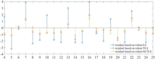
From the results of the three algorithms, robust LS achieved poor accuracy. In fact, it was difficult for the parameter estimation to converge. In the iteration process, because an irrational threshold value of the weight function was obtained and its value was larger than the residual, the algorithm failed in terms of robustness. The traditional robust TLS was more accurate than LS; however, in the process of modifying the stochastic model, each observation datum in the model had a different residual; in this instance, all the observation data No. 4–No. 22 had four residuals. This factor led one observation datum to have different weights. Therefore, although the traditional robust TLS algorithm for the AR model was more precise, its solution was unscientific. Meanwhile, the robust M-TLS proposed in this article overcame the shortcomings of the traditional algorithm, and it was more efficient and precise.

6. Conclusions

A modified solution for parameter estimation for the AR model was proposed in this article. To overcome the shortcomings of traditional solutions based on LS that cannot take into account the observation error in the coefficient matrix, EIV estimation for the AR model was introduced, and by analyzing the current algorithm of robust TLS, the current algorithm based on robust TLS also had unavoidable shortcomings for the AR model. It could not obtain a unique residual for one observation datum; hence, the estimation of the threshold value of the weight function was not scientific. The median function was used to determine a unique residual, and a more rational method for calculating the threshold value was proposed. An iterative algorithm was established using the median function and IGG weight function for the AR model based on EIV estimation. By comparing the proposed algorithm with current algorithms using two examples, the feasibility and efficiency of the proposed algorithm were proved. However, the proposed algorithm also had the shortcoming of increasing the amount of calculation, which needs to be further investigated.

Disclosure statement

No potential conflict of interest was reported by the authors.

Additional information

Funding

This work was supported by the National Natural Science Foundation of China (41601501, 41804029), Natural Science Fund for Colleges and Universities of Jiangsu Province (16KJD420001) and Huaian Key Laboratory of Geographic Information Technology and Applications (HAP201405).

References

- Adcock RJ. 1877. Note on the method of least squares. Analyst. 4(6):183–184.
- Ai-Sharadqah A, Ho KC. 2018. Constrained Cramér-Rao lower bound in errors-in-variables (EIV) models: revisited. Stat Prob Lett. 135(4):118–126.
- Datteo A, Busca G, Quattromani G. 2018. On the use of AR models for SHM: a global sensitivity and uncertainty analysis framework. Reliab Eng Syst Safety. 170:99–115.
- Di Giacinto V. 2006. A generalized space-time ARMA model with an application to regional unemployment analysis in Italy. Int Reg Sci Rev. 29(2):159–198.
- do Nascimento Camelo H, Sergio Lucio P, Vercosa Leal Junior JB, de Carvalho PCM, dos Santos DVG. 2018. Innovative hybrid models for forecasting time series applied in wind generation based on the combination of time series models with artificial neural networks. Energy. 151:347–357.
- Fang X, Li B, Alkhatib H, Zeng W, Yao Y. 2017. Bayesian inference for the errors-in-variables model. Stud Geophys Geod. 61(1):35–52.
- Golub GH, Van Loan CF. 1980. An analysis of the total least squares problem. SIAM J Num Anal. 17(6):883–893.
- Hirata Y, Aihara K. 2017. Improving time series prediction of solar irradiance after sunrise: comparison among three methods for time series prediction. Sol Energy. 149:294–301.
- Huber PJ. 1964. Robust estimation of a location parameter. Ann Math Stat. 35(1):73–101.
- Kurt S, Batu Tunay K. 2015. STARMA models estimation with Kalman filter: the case of regional bank deposits. Procedia-Soc Behav Sci. 195:2537–2547.
- Leyang W, Haiyan L, Yangmao W. 2017. Total least squares method inversion for coseismic slip distribution. Acta Geodaetica et Cartographica Sinica. 46(3):307–315.
- Mahboub V. 2012. On weighted total least-squares for geodetic transformation. J Geod. 86(5):359–367.
- Mahboub V. 2014. Variance component estimation in errors-in-variables models and a rigorous total least-squares approach. Stud Geophys Geod. 58(1):17–40.
- Pfeifer PE, Deutsch SJ. 1980. A three-stage iterative procedure for space-time modeling. Technometrics. 22(1):35–47.
- Pfeifer PE, Ve Bodily SE. 1990. A test of space-time ARMA modeling and forecasting with an application to real estate prices. J Forecast. 16:255–272.
- Rousseeuw P, Wagner J. 1994. Robust regression with a distribution intercept using least median of squares. Comput Stat Data An. 17:65–76.
- Schaffrin B, Wieser A. 2008. On weighted total least-squares adjustment for linear regression. J Geod. 82(7):415–421.
- Schaffrin B, Uzun S. 2011. Error-in-variables for mobile mapping algorithms in the presence of outliers. ISPRS Archives. 22:377–387.
- Shen Y, Li B, Chen Y. 2011. An iterative solution of weighted total least-squares adjustment. J Geod. 85(4):229–238.
- Tuncel KS, Baydogan MG. 2018. Autoregressive forests for multivariate time series modeling. Pattern Recogn. 73:202–215.
- Wan H, Xiao L. 2016. Variational Bayesian learning for robust AR modeling with the presence of sparse impulse noise. DSP. 59:108.
- Wang B, Li J, Liu C. 2016. A robust weighted total least squares algorithm and its geodetic applications. Stud Geophys Geod. 60(2):177–194.
- Yang Y. 1999. Robust estimation of geodetic datum transformation. J Geod. 73(5):268–274.
- Zhangzhen S, Tianhe X. 2012. Prediction of earth rotation parameters based on improved weighted least squares and autoregressive model. Geod Geodyn. 3(3):57–64.