Flash flood risk assessment in urban arid environment: case study of Taibah and Islamic universities’ campuses, Medina, Kingdom of Saudi Arabia

Abstract

Flooding impacts can be reduced through application of suitable hydrological and hydraulic tools to define flood zones in a specific area. This article proposes a risk matrix technique which is applied on a case study of Taibah and Islamic universities catchment in Medina, Kingdom of Saudi Arabia (KSA). The analysis is based on integration of the hydrologic model hydraulic models to delineate the flood inundation zones. A flood risk matrix is developed based on the flood occurrence probability and the associated inundation depth. The risk matrix criterion is classified according to the degree of risks as high, moderate and low. The case study has indicted low to moderate risk for flood frequencies of 5 years return periods and moderate to high risk may exist for flood with rerun period of 50 and 100 years. The results are projected on a two-dimensional satellite images that shows the geographical locations exposed to flooding. A quantitative summary of the results have been presented graphically to estimate the magnitude of the inundation areas that can assess the degree of damage and its economic aspects. The developed flood risk matrix tool is a quantitative tool to assess the damage which is crucial for decision makers.

Keywords:

• Flash floods
• flood risk matrix
• arid regions
• Kingdom of Saudi Arabia (KSA)
• urban areas
• rainfall–runoff modelling
• two-dimensional hydraulic modelling

Introduction

Risk indices and risk matrices are used by governmental agencies for assessing risks and ranking alternative protection measures. The popularity of risk matrices lies in its characteristic to quickly assess risks, as an inexpensive solution. The risk assessment is associated with flood protection as economic, environmental and life safety (Moser 1997; Health and Safety Executive (HSE) 2001). The economic risk assessment is addressed traditionally with cost–benefit analysis, insurance and financial market mechanism. Environmental risks are difficult to determine the evaluation of a flood project, as consequences cannot be directly measured. Social risks are most challenging to quantify; however, the number of fatalities and the cost incurred by damaged infrastructures can be estimated.

Typically, risk assessments are evaluated through geographic information system (GIS), remote sensing and modelling techniques. Sinha et al. (2008) compiled hydrological models with GIS-generated flood risk maps for assessing the potential hazards of Kosi river flood in Nepal and northern India. By integrating geomorphology, land use, land cover and population distribution, and by using the analytical hierarchy process, they were able to construct an index that would help in preparing the mitigation measurements. Zonensein et al. (2008) introduced a flood risk index (FRI) that encompasses both the probability of occurrence of an event and the impacts of the flood on urban areas. Several sub-indices are considered to incorporate flood characteristics and local vulnerabilities. Each sub-index is calculated according to various indicators. The FRI is estimated based on the weighted summation of the sub-indices. The results show that their suggested methodology is a valuable planning tool for decision makers.

Forkuo (2011) demonstrated the utilization of a GIS technique with different data related to land use and population densities for developing a hydrological model in order to depict the flood hazard index map. Their study indicated the usefulness of GIS application in conducting flood hazard studies. Nasiri and Shahmohammadi-Kalalagh (2013) introduced a flood vulnerability index (FVI) as a tool for a flood risk management. The index represented areas that were most vulnerable to flooding, hence needing urgent attention and it also provided more details for taking preventive measurements. Wilkinson et al. (2013) presented 2D risk matrices for analyzing a farm management practice that causes high runoff volumes. Poor farming practices and steep land slopes of agricultural areas can lead to high flood risks. Their study presented a tool for communicating the risk involved with such practices and suggested an alternative planning and management technique to mitigate such risks. The tool was presented to stakeholders and policymakers in order to encourage them for following the suggested practices. Zhang et al. (2015) used the geomorphological unit hydrograph (GUH) technique to develop a distributed hydrological model. Based on the results of the model, three-level risk zones were depicted for a village in China. The risk level was based on the water depth in the area. They showed that the water depth multiplied by the velocity is a better technique to construct the risk zone maps; however; the model did not provide velocities at each node. Finally, they suggested that reliable results can be obtained if accurate digital elevation model (DEM) and advanced numerical techniques are used to solve the hydrodynamic equations. Vojtek and Vojteková (2016) employed GIS, remote sensing and HEC-RAS model to produce flood hazard and flood risk maps. Hazard degree (low, medium or high) was based on the water depth and velocity, while the risk degree was based on the vulnerability of an area. By combining maps with the current and planned urbanization extent, a decision can be made about the accepted level of risk. Thus, the protection to the vulnerable areas could be executed.

Elkharchy (2015) presented a study to produce flood hazards map for the Najran City, KSA. He used hydrological characteristics with a DEM to produce flood hazard index. The resulting maps divided the city into low-, medium- and high-risk zones. He concluded that a better identification of each zone depends on a high-resolution DEM. Moreover, updated land use maps and DEM are required to update the risk zones since the construction of new residential areas is at a high rate. Sharif et al. (2016) presented a study, representing a flood hazard map for the city of Riyadh, KSA. The north of the city is undergoing a rapid urbanization within an Al-Aysen watershed. Hydrologic and hydraulic modelling with the integration of remote sensing and GIS techniques were employed for producing risk zone maps. The authors indicated that the lack of detailed rainfall data is the reason of inaccurate results in the study area. However, the obtained results are useful for planning flood drainage and prevention measures. Winter et al. (2018) studied uncertainties in flood risk models. Five variables, within the hydrologic and risk models, were studied. Sensitivity analysis of the flood risk model with respect to the five variables was performed. They concluded that the result of a flood risk model is subjective to the selected values of variables and the better estimation of such values indicates a better decision-making process.

This article presents a flood risk matrix technique for assessing risks in urban arid regions. The technique is demonstrated through its application on a case study of the protection channel in the catchment of Taibah and Islamic universities (TU and IU) in Medina, KSA. The study focuses on assessing the impacts of inundation depths resulting from flash floods on the flood channel and the floodplains of the channel for different frequencies ranging from 5- to 100-year return periods using HEC-HMS hydrologic and 2D HEC-RAS hydraulic modelling techniques in order to delineate the inundation area at different degrees of flood hazards.

Study area case study

The study area is comprised of 34 km² drainage area, a tributary of Wadi Al-Aqiq. It is located within the vicinity of longitude N 24^° 28.788' and latitude E 39^° 32.767’, which covers an upstream area of TU and IU campuses in Medina, the western region of KSA. Figure 1 shows Medina region in relation to KSA (left image), the enlarged Medina region (right top image) and location of the study area (TU and IU campuses, bottom right image).

Figure 1. Location of the study area in relation to KSA and the western region (modified from Abdulrazzak et al. 2018b).

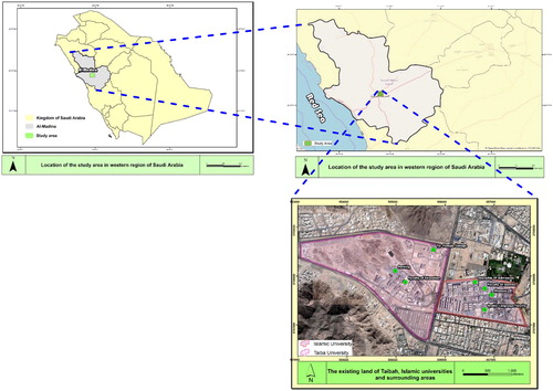
The topography is characterized by a gentle slope surrounded by relatively high mountains in the upstream area (in the west) and a relatively flat area in the downstream part (in the east). The geology mostly consists of a barren surface with hard igneous and metamorphic rocks. The surface rocks and barren vegetation in some parts of the upstream area have a limited exposure. The catchment hills cover both campuses and the downstream area. The ground elevation varies from 533 m to 966 m above the mean sea level. The average catchment slope is 1%, orientated from west to east direction towards the downstream of Wadi Al-Aqiq’s main channel. Infrastructures, such as buildings, roads and some urban developments at upstream, cover a large portion of the catchment, especially at the areas close to Wadi Al-Aqiq’s main channel.

Methodology

The methodology for conducting the flood risk assessment consists of the watershed delineation, the land use analysis for estimating the curve number (SCS-CN) using remote sensing techniques and the analysis of rainfall depths for estimating the design rainfall depths from the data available at rainfall stations in the study area. The rainfall–runoff modelling was achieved using the HEC-HMS software program in order to get design hydrographs for different return periods (ranges from 5 to 200 years). The developed hydrographs are used in the 2D HEC-RAS model to estimate the inundation flood depths and their areal coverage. Based on previous analyses (Moser 1997; Elfeki et al. 2017; Elfeki and Bahrawi 2017; Abdulrazzak et al. 2018a; Elfeki et al. 2018), a flood risk matrix is used to delineate the degree of flood hazards and the locations of the most vulnerable areas. A quantitative approach is followed to estimate the damage at different flood risk levels (Moser 1997). The details of the aforementioned steps are given below.

Watershed delineation

The Aquaveo Watershed Modeling System (WMS) software has been applied for rainfall–runoff watershed modelling in different parts of the world, including KSA. In this study, the WMS software was applied for delineating the watershed in the study area using a DEM of 30 m resolution. The obtained information was used as one of the inputs for applying the HEC-HMS model to generate the inflow flood hydrograph. Figure 2 shows the watershed delineated and land cover features projected on the topographic map of the study area and nearby urban developments. The figure indicates that the streams extracted from the DEM match with the streams presented in the topographic map. The geomorphological parameters of the catchment obtained from the WMS are shown in Table 1.

Figure 2. Watershed delineation and stream network projected on a topographic map (a), and the land use and land cover map of the watershed based on a remote sensing technique for the estimation of CN (b).

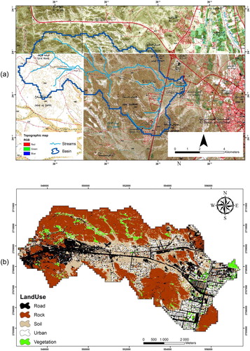
Table 1. Geometric and morphological parameters.

Parameter	Simple Abbr.	Unit	Value
Basin area	A	Km^2	34.22
Basin slope	BS	Km/Km	0.101
Maximum flow distance	MFD	Km	13.197
Maximum flow slope	MFS	Km/Km	0.011
Centroid stream distance	CSD	Km	6.41
Centroid stream slope	CSS	Km/Km	0.007
South aspect ratio	%SF	%	0.49
North aspect ratio	%NF	%	0.51
Maximum stream length	MSL	Km	12.26
Maximum stream slope	MSS	Km/Km	0.01
Basin length	L	Km	10.8
Shape factor	Shape	m^2/m^2	3.42
Sinuosity factor	Sin	m/m	1.13
Perimeter	P	Km	40.81
Mean basin elevation	AVEL	Km	694.1
Basin centroid X		m	552158
Basin centroid Y		m	2708342

Land use and land cover analysis and SCS-CN estimation

Land use and land cover maps of the study area (shown in Figure 2) were prepared using a remote sensing technique for classifying the Image Sentinel-2 with the resolution of 10 m by 10 m, provided by the ESA (European Space Agency). Maximum likelihood classification is one of the most common supervised classification techniques. This technique is employed using ENVI software. With this approach, the researchers developed the spectral responses of known categories, such as urban areas, roads, rocks (training class). The software allocated each pixel in the image to the different types of land cover where its spectral response is most similar. This classification was accompanied with a field survey, providing information about the different types of land covers (Priess et al. 2013; Gaubi et al. 2016). In this study, Google Earth image was used as a reference image. Random ground truth points were collected, using hand-held GPS receiver for assessing classification. An accuracy assessment is used to evaluate the resulting classified map using training sites. The kappa coefficient was 86%, which means that this classification is acceptable (Ozsoy et al. 2012; Gaubi et al. 2016). Five land use classes were identified that consist of vegetation, urban areas, road, soil and rocks as shown in Table 2. The table shows the CN value for each category and the computed composite CN value for the watershed.

Table 2. Computed composite SCS-CN for the watershed.

Land cover and land use features	SCS-CN	Area (km^2)	Composite CN
Urban roads	98	8.61	86.1
Vegetation	60	0.83
Rocks	95	14.76
Soil alluvium	65	10.02

Rainfall analysis

Two rainfall stations in the vicinity of the watershed, namely: M001 and M103 (shown in Figure 3), with a record length of more than 40 years, were used in the analyses. Rainfall frequency analysis was performed on the data. The theoretical frequency distributions, namely: normal, Gumbel, two- and three-parameter log-normal, Pearson type III and log-Pearson type III, are used (Haan 1977; Kite 1978). Figure 4 (top part) shows the fitting of the aforementioned theoretical probability distributions to the data. The best distribution method that fitted the data from the stations M001 and M103 are the two-parameter log-normal and the three-parameter log-normal, respectively, based on the root mean square error (RMSE) criterion (Haan 1977). The RMSE is tabulated in Table 3. Figure 4 (bottom part) shows the best distribution method for both stations. The predicted rainfall depths for different return periods of 5, 10, 25, 50, 100 and 200 years are presented in Table 4. The average rainfall depth over the watershed was calculated using the inverse square distance weighting method (Viessman et al. 1977). The average rainfall depth over the watershed is also shown in Table 4. The disaggregation of the design rainfall depth was achieved through the application of the method developed by Elfeki et al. (2014), as shown in Figure 5(a). The method is suitable for the areas where thunderstorms occur dominantly and the peak burst of the precipitation is close to the start of the storm. This temporal rainfall distribution pattern was found to be suitable for the arid region, covering most parts of KSA (Ewea et al. 2016). The temporal pattern is different from the temporal pattern resulting from the cyclonic-type storms, where the peak burst occurs in the middle of the distribution, such as the one developed for the United States (humid region), known as SCS type II distribution.

Figure 3. Rainfall stations in the study area: M001 and M103.

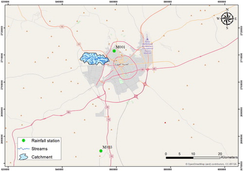
Figure 4. Fitting probability distributions to the maximum daily rainfall: a left column for station M001 and a right column for station M103.

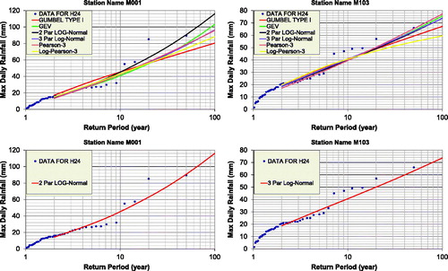
Figure 5. Results of the rainfall–runoff model (HEC-HMS): (a) cumulative rainfall distribution for 3-h duration and (b) the corresponding hydrographs for different return periods.

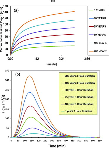
Table 3. RMSE for theoretical statistical distributions used to fit the rainfall data (modified from Abdulrazzak et al. 2018b).

Distribution type	RMSE (M001) (mm)	RMSE (M103) (mm)
Gumbel type 1	15.17	5.72
Generalized extreme value (GEV)	12.17	4.64
Two-parameter log-normal	7.92	5.02
Three-parameter log-normal	12.19	4.56
Pearson type III	11.6	4.57
Log-Pearson type III	13.56	7.59

Boldface numbers are the minimum RMSE which corresponds to the best distribution.

Table 4. Design rainfall for the study area.

Station	5 Years	10 Years	25 Years	50 Years	100 Years	200 Years
M001	30.44	45.24	69.04	90.71	115.96	145.19
M103	31.36	40.61	53.18	63.15	73.6	84.59
Average*	30.5	45	68.2	89.2	113.7	142

*Based on inverse distance squared weighting.

Rainfall–runoff modelling

It is a normal practice to apply synthetic unit hydrograph (SUH) methods for ungagged catchments where recorded runoff is unavailable. The SCS curve number (SCS-CN) method is applied to estimate the excess rainfall depth, which in turn is used to estimate the direct runoff. The method is widely used all over the world, including the arid regions (Mishra and Singh 2003). The WMS software is usually used in combination with the application of the most popular hydrological model, HEC-HMS). The HEC-HMS model has been used successfully in different parts of the world in order to evaluate and simulate the rainfall–runoff process over the dendritic watershed. The HEC-HMS model depends on two major inputs: watershed physical feature and the hydrological information. Figure 5(a) shows the design cumulative rainfall distribution patterns for different return periods, while Figure 5(b) shows the simulated flood hydrograph for different return periods that corresponds to the rainfall distribution in Figure 5(a). Table 5 presents the summary of the rainfall depth, losses, effective rainfall depth and the computed runoff characteristics including runoff volume, peak discharge and time to peak from the HEC-HMS model for different return periods. These results are used later on for the hydraulic model.

Table 5. Summary of rainfall–runoff model based on the HEC-HMS simulation.

Item	5 Years	10 Years	25 Years	50 Years	100 Years	200 Years
Rainfall depth (mm)	30.5	45.0	68.2	89.2	113.7	142.0
Loss depth (mm)	23.8	29.08	34.26	37.24	39.62	41.52
Effective rainfall (mm)	6.68	15.97	33.93	51.99	74.07	100.48
Peak discharge (m^3/sec)	20.5	49.4	106.4	164.5	236.4	323
Runoff volume (m^3)	2,286	5,466	1,161	1,779	25,342	34,377
Time to Peak (h)	2:45	2:35	2:25	2:20	2:15	2:15

Hydraulic flood modelling

This section deals with the 2D hydraulic modelling using the 2D HEC-RAS model for the flood channel in the TU and IU catchment. The DEM, developed by King Abdul-Aziz City for Science and Technology (KACST) with 0.5 m resolution, supported by satellite images for urban areas in Medina, was used for the hydraulic modelling. The hydraulic simulation was carried out for an unsteady state condition to estimate the water surface elevations using the inflow hydrograph for the selected return periods, presented in Figure 5(b). This resulted in the generation of maps representing flood inundation depths at different flood frequencies or return periods of 5, 50 and 100 years, respectively.

The 2D simulation for 5-year return period (Figure 6, top part) estimated the maximum water depth of 4.65 m for IU and 7.33 m for TU, represented by red colour. The minimum water depth is 0.00001 m (boundary limit), represented by dark blue colour. Flood inundation mapping of 2D hydraulic modelling of the flood channel in the TU and IU catchment for 5-year return period is shown in Figure 6 (top row). This figure shows no spread of water in the floodplains except at the end of the channel.

Figure 6. Results of flooding from a 2D HEC-RAS model: Taibah (left images) and Islamic (right images) universities.

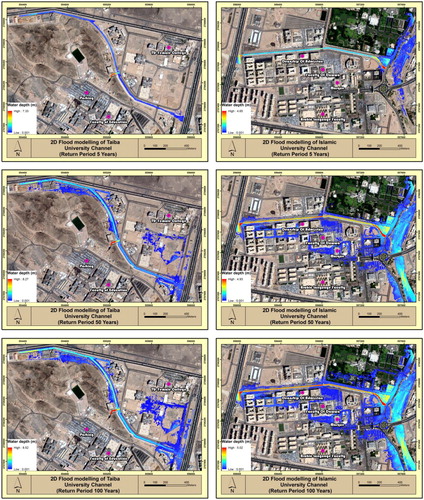
For a 50-year return period, the flood inundation mapping of the 2 D hydraulic modelling is shown in Figure 6 (middle row). More spreading is observed around the buildings; however, the excessive spreading is observed at the end of the channel. The estimated maximum water depth is 4.93 m for IU and 8.27 m for TU, respectively. For a 100-year return period, the flood inundation mapping of the 2D hydraulic modelling is shown in Figure 6 (last row). More spreading is observed around the buildings; however, the excessive spreading is observed at the end of the channel. The estimated maximum water depth is 5.02 m for IU and 8.52 m for TU, respectively. The results indicated that the maximum depth in TU is higher than that of the IU channel. This is because of the reason that a deep pit is located nearby the TU channel. The flow fills the pit when passes through this portion of the channel, which results in producing high water depths. Results also indicated that no floodwater flowing over the land would be observed for the return period of 5 years. However, the flood will be significant and dominant for the return period of 50 years and maximum impacts will be observed for the return period of 100 years.

Flood risk assessment

A typical risk matrix is constructed, which is modified from FEMA (2004), as shown in Table 6. In this table, the left column is the likelihood of occurrence, which is classified based on an ordinal scale using terms, such as rare, unlikely, likely. The ordinal scale is transferred in a return period as rare (more than 100-year return period), unlikely (100-year return period), possible (50-year return period), very likely (5-year return period) and almost certain (less than 5-year return period). In the top horizontal row of Table 6, the consequences related to the risks are classified using the terms, namely: low, minor, major, sever and catastrophic. These consequences are evaluated according to the flood depths above the ground surface. We used (low: depth less than 0.1 m, minor: depth between 0.1 and 0.5 m, major: depth between 0.5 and 1.0 m, sever: depth between 1.0 and 2.0 m and catastrophic: depth >2.0 m). We formulated a table, where each cell in the table is assigned a degree of risk such as low, medium and/or high, represented by specific colour like green, yellow and red.

Table 6. Flood risk matrix.

Risks of low likelihood and low consequences are thought to be acceptable. Risks of high likelihood and high consequences are believed to be rejected by the society and thus, intolerable. Between these two boundaries, lies a region of tolerable risk (but not acceptable), which should be continually appraised and made ‘as low as reasonably practicable’ (ALARP) (FEMA 2004). This ALARP criterion essentially requires a benefit–cost analysis approach for judging the burden of further risk reductions against their benefit.

Results and discussion

The matrix in Table 6 was applied to assess the risk levels at the universities’ campuses and the results are displayed in Figure 7 for 5-, 50- and 100-year return periods. The matrix results provide the information of risk levels that can be used for solving flood problems alternatively. Figure 7 represents flood risk maps for the flood protection channel of the TU and IU catchment and its surroundings for 5-, 50- and 100-year return periods. Red colour zones indicate the high priority areas that need immediate actions for the implementation of flood mitigation measures, while the yellow colour zone indicates the relatively low priority areas. The green zones do not pose a serious hazard, as the existing channel capacity can accommodate the simulated flood depths. Red colour zones expand as the return period increases from 5 to 100 years due to the increase in the flood water depths in relation to the channel capacity. The risk matrix based on the flood inundation maps indicates the redesign of the channel for 100-year flood. Another alternative solution is to elevate the channel banks to accommodate the 100-year flood.

Figure 7. Application of the flood risk matrix based on the flooding in the TU (left images) and IU (right images) catchment.

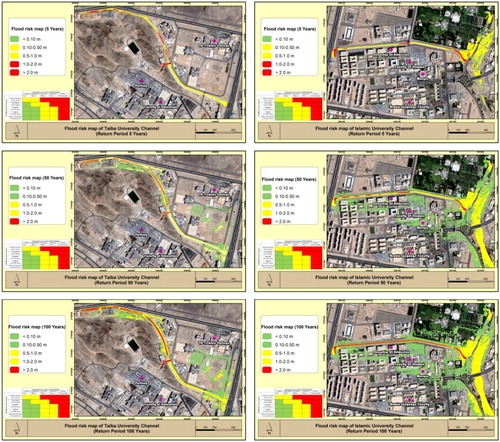
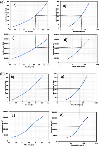
The aforementioned results presented in Figure 7 show the locations of high, low and medium risks visually. The priority action plan is also evident for the decision makers in Figure 7. However, a more quantitative analysis is also essential to transfer the results into a global summary that can be later transferred into money and cost–benefit analysis can be applied (Moser 1997). Figure 8(a) and 8(b) display the summary of results obtained from the above analysis, performed for the channel in the TU and IU catchment. The logic for assessment in the figures starts from the top-right corner (a) where the peak discharge versus the return periods relationship is derived from the hydrological analysis. The left-top corner (b) represents the rating curve or the maximum stage peak discharge relationship. The subsequent figure in the bottom-left corner (c) shows the transformation of the maximum stage into the corresponding inundation area. The fourth figure in the bottom-right corner (d) shows the return period of the corresponding inundation area, which describes the risk of the inundation area due to the specific design flood. This figure can be transferred to an economic value based on the value of the land and the properties in the region. The damage can be evaluated in terms of money to help the decision maker for adopting the mitigation measures that are required in the particular area.

Figure 8. (a) Quantitative summary of risk results for the TU channel. The logic for risk assessment in this figure flows counterclockwise starting from (a) and ending at (d). (b) Quantitative summary of risk results for the IU channel. The logic for risk assessment in this figure flows counterclockwise starting from (a) and ending at (d).

Conclusions

The proposed flood risk matrix technique for the assessments of flood risks in the urbanized arid environment was applied on a case study of the TU and IU catchment in Medina, KSA. Results of the risk matrix are visualized in 2D satellite images, showing the geographical locations influenced by the flood coverage. It indicated low-to-moderate risk for a flood frequency of 5-year return period and moderate-to-high risk for flood with return periods of 50 and 100 years. A quantitative summary of the results is shown graphically to estimate the magnitude of inundation areas, which can be later transferred into a degree of damage. The proposed risk matrix technique is in line with the main principles reported in the literature (FEMA 2004) that may provide an appropriate tool for arid and extreme arid regions. The technique needs further evaluation through applications to other case studies.

Recommendations for flood mitigations in the study area

The proposed recommendations are twofold: structural and non-structural measures. Several structural measures are proposed. In the upstream area, it is suggested to build a check dam on one of the upstream branches of the watershed. This dam will reduce the peak flow of the watershed. Moreover, cross-wadi retardation structures are suggested, and rehabilitation of the upstream portion of the flood earthen channel is proposed using riprap. In the downstream area, it is proposed to redesign the flood protection channel in order to accommodate the 100-year flood (either by elevating the sides of the channel banks or by deepening the channel bed) and removal of buildings near the channel. Another measure that needs to be adopted is an alternative alignment of the channel where the new path and the size of the channel would ensure the safety of the two universities against the 100-year flood. Non-structural measures can also be considered as a set of mitigation and/or adaptation measures that do not make use of traditional structural flood defence measures. It can be very cost-effective when compared to structural measures. A particular advantage when compared to structural measures is its ability of sustainability over a long term with minimal costs for operation, maintenance, repair, rehabilitation and replacement.

Some of other protection measures are proper safe elevation of buildings in the area near the channel, reallocation and delineation of people evacuation area, the use of wet flood proofing and dry flood proofing for the construction of new buildings, flood emergency preparedness plans, land use regulations, instantiation of flood warning system (real-time wireless automatic wearing systems), an adaptation of effective building codes for the existing and planned facilitates and design of the public education programme. Implementation of these measures depends on the decision maker’s political will, protection levels needed against flood damages, and cost and the environmental impact assessment.

Acknowledgement

The authors would like to thank the anonymous reviewers for appreciation of the work and their valuable comments.

Disclosure statement

No potential conflict of interest was reported by the authors.

Additional information

Funding

This article is one of the outcomes of KASCT funded research project ART 34-46. Appreciate KACST funding of the project.

References

- Abdulrazzak M, Al-Shabani A, Noor K, Elfeki A, Kamis A. 2018a. Integrating hydrological and hydraulic modelling for flood risk management in a high-resolution urbanized area: case study Taibah University Campus, KSA. Recent advances in environmental science from the Euro-Mediterranean and surrounding regions, 01/2018, Cham: Springer, pp. 827–829; ISBN: 978-3-319-70547-7, DOI:10.1007/978-3-319-70548-4_243
- Abdulrazzak M, EA, Kamis AS, Kassab M, Alamri N. 2018b. Flood mitigation in Taibah and Islamic universities campuses and downstream areas, Medina. King Abdulaziz City for Science and Technology (KACST). Unpublished Final Report. Cham: Springer.
- Elfeki A, Al-Shabani A, Bahrawi J, Alzahrani S. 2018. Quick urban flood risk assessment in arid environment using HECRAS and dam break theory: case study of Daghbag Dam in Jeddah, Saudi Arabia. Recent Advances in Environmental Science from the Euro-Mediterranean and Surrounding Regions, 01/2018, Cham: Springer, pp. 1917–1919; ISBN: 978-3-319-70547-7, DOI:10.1007/978-3-319-70548-4_553
- Elfeki A, Bahrawi J. 2017. Application of the random walk theory for simulation of flood hazards: Jeddah flood 25 November 2009. IJEM. 13(2):169–182.
- Elfeki AM, Ewea HA, Al-Amri NS. 2014. Development of storm hyetographs for flood forecasting in the Kingdom of Saudi Arabia. Arab J Geosci. 7(10):4387–4398.
- Elfeki A, Masoud M, Niyazi B. 2017. Integrated rainfall-runoff and flood inundation modeling for flash flood risk assessment under data scarcity in arid regions: Wadi Fatimah basin case study, Saudi Arabia. Nat Haz. 85(1):87–109.
- Elkharchy I. 2015. Flash flood hazard mapping using satellite images and GIS tools: a case study of Najran City, Kingdom of Saudi Arabia (KSA). Egypt J Remote Sens Space Sci. 18:216–278.
- Ewea HA, Elfeki AM, Bahrawi JA, Al-Amri NS. 2016. Sensitivity analysis of runoff hydrographs due to temporal rainfall patterns in Makkah Al-Mukkramah region, Saudi Arabia. Arab J Geosci. 9:424.
- FEMA. 2004. HAZUS-MH. FEMA’s methodology for estimating potential losses from disasters. US Federal Emergency Management Agency. http://www.fema.gov/plan/prevent/hazus/index.shtm
- Forkuo EK. 2011. Flood hazard mapping using Aster Image data with GIS. Int J Geomat Geosci. 1(4):932–950.
- Gaubi I, Chaabani A, Ben Mammou A, Hamza MH. 2016. A GIS-based soil erosion prediction using the revised universal soil loss equation (RUSLE) (Lebna watershed, Cap Bon, Tunisia). Nat. Hazards, 86(1):219–239. DOI: 10.1007/s11069-016-2684-3.
- Haan CT. 1977. Statistical methods in hydrology. Ames, IA: Iowa State University Press.
- Health and Safety Executive (HSE). 2001. Reducing risks, protecting people – HSE’s decision making process. London: HMSO.
- Kite GW. 1978. Frequency and risk analyses in hydrology. 2nd ed. Littleton, CO: Water Resources.
- Mishra SK, Singh VP. 2003. SCS-CN method. Part-II, analytical treatment. Acta Geo-Phys Polon. 51(1):107–123.
- Moser DA. 1997. The use of risk analysis by the U.S. Army Corps of Engineers . Alexandria, VA: Institute for Water Resources, USACE. p. 34.
- Nasiri H, Shahmohammadi-Kalalagh S. 2013. Flood vulnerability index as a knowledge base for flood risk assessment in urban area. J Nov Appl Sci. 2(8):266–269.
- Ozsoy G, Aksoy E, Dirim MS, Tumsavas Z. 2012. Determination of soil erosion risk in the Mustafakemalpasa River Basin, Turkey, using the revised universal soil loss equation, geographic information system, and remote sensing. Environ Manag. 50(4):679–694.
- Priess JA, Schweitzer C, Batkhishig O, Koschitzki T, Wurbs D. 2013. Impacts of agricultural land-use dynamics on erosion risks and options for land and water management in Northern Mongolia. Environ Earth Sci. 73(2): 697–708. doi:10.1007/s12665-014-3380-9
- Sharif HO, Al-Juaidi FH, Al-Othman A, Al-Dousary I, Fadda E, Jamal-Uddeen S, Elhassan A. 2016. Flood hazards in an urbanizing watershed in Riyadh, Saudi Arabia. Geomat Nat Haz Risk. 7(2):702–720.
- Sinha R, Bapalu GV, Singh LK, Rath B. 2008. Flood risk analysis in the Kosi river basin, north Bihar using multi-parametric approach of analytical hierarchy process (AHP). J Indian Soc Remote Sens. 36(4):335–349.
- US Army Corps of Engineers HEC-HMS. 2016. http://www.hec.usace.army.mil/software/hec-hms/
- US Army Corps of Engineers HEC-RAS. 2016. http://www.hec.usace.army.mil/software/hec-ras/
- Viessman W, Knapp JW, Lewis GR, Harbaugh TE. 1977. Introduction to hydrology. 2nd ed. New York: Harper & Row.
- Vojtek M, Vojteková J. 2016. Flood hazard and flood risk assessment at the local spatial scale: a case study. Geomat Nat Haz Risk. 7(6):1973–1992.
- Wilkinson ME, Quinn PF, Hewett CJM. 2013. The floods and agriculture risk matrix: a decision support tool for effectively communicating flood risk from farmed landscapes. Int J River Basin Manag. 11(3):237–252.
- Winter B, Schneeberger K, Huttenlau M, Stötter J. 2018. Sources of uncertainty in a probabilistic flood risk model. Nat Haz. 91(2):431–446.
- Zhang D-W, Quan J, Zhang H-B, Wang F, Wang H, He X-y. 2015. Flash flood hazard mapping: a pilot case study in Xiapu River Basin, China. Water Sci Eng. 8(3):195–204.
- Zonensein J, Miguez MG, Magalhaes LPC, Valentin MG, Mascarenhhas FCB. 2008. Flood risk index as an urban management tool, 11th International Conference on Urban Drainage. Edinburgh, Scotland, UK: IWA.