The Method of Fundamental Solutions for Solving the Inverse Problem of Magma Source Characterization

Abstract

Volcano is one of the geodynamic phenomena causing irreparable damages. As lava accumulates in reservoir and then comes to the surface, geometry of the source can be used to predict volcanic eruptions. In this study, using the inverse method of fundamental solutions (MFS) and taking into account the effect of topography, the geometry of the source including shape, depth and centre position of the magma tank is estimated. The MFS is a numerical method for solving boundary value problems with known partial differential equations. The displacement field calculated in the previous studies using InSAR for deflation mode of Cerro Blanco volcano was utilized in this study. It was estimated that the magma source of the volcano is a sphere with a radius of 1 km located at a horizontal position of ($1.001\pm 4e-6,-1.001\pm 1e-6$) km and the depth of about 10 km from the summit with respect to the defined coordinate system. This finding is consistent with that of recent studies in which inversion of InSAR data was used to analyse the geometry of the magma source. The RMSE between the deformation fields of the magma source calculated in the previous studies and that of the study herein via MFS was approximately 3 mm.

Keywords:

• Magma source
• inverse MFS
• boundary value problem
• meshless method
• volcano

1. Introduction

Understanding the geometry of magma reservoir and ground deformation is essential in predicting volcanic eruption and therefore in minimizing damage to human lives and livelihood. Many studies have been done in this area. For example, Carbone et al. (2008) used pairs of microgravity and levelling surveys and electronic distance metre (EDM) measurements during the flank eruption of Etna in 1981 whereby modelled the intrusive mechanism of the volcano. Beauducel et al. (2004) modelled surface deformation and geometry of volcano magma reservoir of CampiFlegrei using boundary element method (BEM). Latimer et al. (2010) calculated the magma source of Auckland volcanic region using radar waves and genetic algorithm (GA). Saltogianni and Stiros (2013) provided a new algorithm for modelling of magma source which avoids local minima. They carried out the modelling using data from Santorini volcano in Greece. Delgado et al. (2014) studied the movement of Hudson volcano in Chile using interferometric synthetic aperture radar (InSAR) observations. Shirzaei and Walter (2009) calculated the source of deformation in CampiFlegrei using GA and simulated annealing (SA) algorithms. Because of the high level of risk posed to human lives in volcanic areas, many studies have been done in this field in recent years (Carbone et al. 2007; Riguzzi et al. 2012; Field et al. 2012; Nakao et al. 2013; Rodríguez et al. 2015; Ulloa et al. 2016; Camiz et al. 2017; Prezzi et al. 2017). In the majority of studies, the effect of topography has not been considered. In this study, however, using the method of inverse MFS, the geometry of the Cerro Blanco volcano magma source is estimated considering the effect of real topography. This is a novel application of the inverse MFS in geodynamics.

MFS is a meshless boundary method applicable to certain boundary value problems and initial/boundary value problems (Golberg, 1995; Karageorghis et al. 2011b, 2013; Bin-Mohsin and Lesnic, 2017). Since its introduction as a numerical method, the method has become increasingly popular. This popularity is primarily due to the ease with which the MFS can be implemented in problems in various geometries, particularly three-dimensional problems. The advantages that the MFS has over the more classical domain or boundary discretization methods are discussed here. First, the MFS is a meshless method meaning that instead of mesh a mere collection of points is required for discretization of a domain. Second, it does not involve integration which could potentially be troublesome and complicated, as is the case with, for example, BEM. Finally, it is a boundary method which means that it shares all the advantages that the BEM has over domain discretization methods such as the finite-element method (FEM) or finite difference method (FDM). In addition to the benefits mentioned herein, unlike methods such as FEM, 3 D MFS does not need the very time consuming 3 D mesh generation. In mesh-based numerical methods, human interference can never be completely eliminated from the process of mesh generation (Mossaiby et al. 2016). As a result, the MFS is ideally suited for the solution of problems in which the boundary is of major importance or requires special attention (Karageorghis et al. 2011b).

The drawbacks of the MFS are as follows. First, the fundamental solution (MFS) of the partial differential equation has to be explicitly known. Next, it often leads to severely ill-conditioned linear system of equations, especially when the external sources are far from the boundary. On the other hand, if they are too close to the boundary, numerical singularities may arise in the approximate solution. Finally, the proper definition of the location of sources is not a trivial task in general, and may lead to a non-linear optimization problem if it needs to be done in an automated way.

Inverse problems are in this category. In recent years, MFS is widely used in numerical solution of inverse problems. A general assessment of the applications of this method in inverse problems is given in Fairweather and Karageorghis (1998). The most complicated class of inverse problems is called geometrical inverse problems where the place and shape of part of the boundary is unknown and should be calculated. MFS for the first time was applied to solve geometrical inverse problems in linear elasticity (Alves and Martins, 2009). Recent application of inverse MFS can be found in Borman et al. (2009), Karageorghis and Lesnic (2009), Karageorghis et al. (2013) and Marin and Cipu (2017).

In this study considering the earth with its topography as a homogeneous isotropic medium with linear elasticity, for the first time the shape and the position of magma reservoir is calculated using three-dimensional inverse MFS. Inverse MFS is introduced in the second section and the application of MFS in determination of magma source is discussed. In the third section, the study areas and the data set used in this study are presented. In the fourth section, the MFS is executed on a simulated area. Then, the results of the numerical analyses performed on the Cerro Blanco data set are discussed. In the final section, the conclusions of the study are presented.

2. Method of fundamental solution for geometric inverse problem

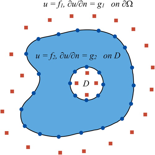
In an elastic domain Ω, sometimes it is intended to determine an unknown cavity $D\subset \Omega$ using boundary measurements taken on the border $\partial \Omega$ (Figure 1). This situation commonly arises, for instance, in fracture mechanics when some defects stem from the manufacturing processes, or when the elastic properties of the material deteriorate due to possible damages a product endures throughout the manufacturing processes. Another application of the MFS is shown in the current study to solve a problem of paramount importance for the geodesians.

Figure 1. A symbolic domain Ω, cavity D, boundary conditions and source (square) and boundary (circle) points.

Suppose partial differential equation (PDE) (1) $$\mathcal{L}\left(u\right)=0$$(1) subject to the boundary conditions (2) $$u=f_1\hspace{1em}\text{and}\hspace{1em}\partial \left(u\right)/\partial \left(\mathbf{n}\right)=g_1\hspace{1em}\text{on} \partial \Omega$$(2) and (3) $$u=f_2\hspace{1em}\text{and}\hspace{1em}\partial \left(u\right)/\partial \left(\mathbf{n}\right)=g_2\hspace{1em}\text{on} \partial D$$(3) where $\mathcal{L}$ is a linear differential operator with constant coefficients and u is an unknown parameter which should be estimated. $f_1,f_2,g_1,\text{\hspace{0.5em}and\hspace{0.5em}}{g}_2$ are boundary values. n is the outward unit normal vector on the boundary. An approximation which satisfies both the governing partial differential equation (PDE) and the boundary condition (at a finite number of points) is constructed in the MFS. The MFS of Equation (1)(1) $$\mathcal{L}\left(u\right)=0$$(1) satisfies Equation (4)(4) $$\mathcal{L}\left(G\right)=\delta (P-Q)$$(4) . (4) $$\mathcal{L}\left(G\right)=\delta (P-Q)$$(4) where δ is the Dirac delta function, Q is the source point and P is the boundary point. If the source point Q is placed outside the domain Ω, then the MFS G(P, Q) and any linear combination of MFS satisfies Equation (1)(1) $$\mathcal{L}\left(u\right)=0$$(1) without any singularity. Hence, an approximation to Equation (1)(1) $$\mathcal{L}\left(u\right)=0$$(1) is constructed in the form of Equation (5)(5) $$u\left(P\right)=\sum _{d=1}^2\sum _{n=1}^N\left(c_n^{d}G(P,Q_n^d)\right)$$(5) . (5) $$u\left(P\right)=\sum _{d=1}^2\sum _{n=1}^N\left(c_n^{d}G(P,Q_n^d)\right)$$(5) where ${(Q_n^d)}_{n=1,\dots ,N,d=1,2}$ represent source points placed outside the domain $\Omega (d=1)$ and inside $D(d=2),{(c_n^d)}_{n=1,\dots ,N,d=1,2}$ are constant coefficients and u is the boundary value at point P. Figure 1 is a schematic representation of the boundary and the source point distribution.

To determine constants coefficients and the cavity geometry in MFS, boundary points (circles in Figure 1) and boundary conditions for Equation (5)(5) $$u\left(P\right)=\sum _{d=1}^2\sum _{n=1}^N\left(c_n^{d}G(P,Q_n^d)\right)$$(5) are used in a system of nonlinear equations. Once the constants and cavity parameters are determined, the value of u at any point within the domain can be calculated using suitable MFS between that specific point and the source points.

2.1. Application of inverse MFS in determination of magma source

Considering a three-dimensional homogeneous isotropic domain Ω with a cavity D in as a volcanic field and magma source, respectively, the goal here is to determine the geometry of the magma source. In the absence of body forces, the governing equations of equilibrium for a homogeneous isotropic linear elastic solid are the Cauchy–Navier equations (Equation 6(6) $$(\lambda +\mu )u_{k,ki}+\mu u_{i,kk}=0$$(6) ). (6) $$(\lambda +\mu )u_{k,ki}+\mu u_{i,kk}=0$$(6) where λ and μ are the Lam elastic constants, summation over repeated subscripts is implied and partial derivatives are of displacement nature shown in Equation (7)(7) $$u_{i,j}=\partial \left(u_i\right)/\partial \left(x_j\right)$$(7) . (7) $$u_{i,j}=\partial \left(u_i\right)/\partial \left(x_j\right)$$(7) subject to the Cauchy boundary conditions on the outer boundary $\partial \Omega$ (8) $$\begin{array}{c}{u}_i=f_i,\hspace{1em}i=1,2,3\hfill \\ t_i=g_i,\hspace{1em}i=1,2,3\hfill \end{array}$$(8) where u_i, t_i are the displacements and tractions, respectively, and Neumann condition on the inner boundary $\partial D$ (9) $$t_i=0,\hspace{1em}i=1,2,3$$(9) where f_i and g_i are known displacements and tractions, respectively. According to Karageorghis et al. (2011a) Dirichlet boundary condition is used on the internal borders that are a rigid inclusion and Neumann boundary condition of Equation (9)(9) $$t_i=0,\hspace{1em}i=1,2,3$$(9) is used for cavity. Accordingly, in the problem subject of this study the Neumann boundary condition was used. In the linear theory, the strains ${\epsilon }_{ij},i,j=1,2,3$, are related to the displacement gradients as demonstrated by the following equation: (10) $${\epsilon }_{ij}=\frac{1}{2}\left(\frac{\partial u_i}{\partial x_j}+\frac{\partial u_j}{\partial x_i}\right)$$(10) and the stresses ${\sigma }_{ij},i,j=1,2,3$, are given in Equation (11)(11) $${\sigma }_{ij}=\lambda {\delta }_{ij}{u}_{k,k}+2{\epsilon }_{ij}\mu$$(11) (11) $${\sigma }_{ij}=\lambda {\delta }_{ij}{u}_{k,k}+2{\epsilon }_{ij}\mu$$(11) where δ_ij is the Kronecker delta. The tractions $t_j,j=1,2,3$ are defined in terms of the stresses as the following equation: (12) $$t_i={\sigma }_{ij}{n}_j$$(12) where $n_1,n_2,\text{\hspace{0.17em}and\hspace{0.17em}}{n}_3$ denote the coordinates of the outward normal to the boundary. Surface displacement in and around topographic configuration comes from the interaction of the ground surface and perturbed displacement field (Luzón et al. 1997). Hence, the total motion may be explained as the superposition of the free-field displacement $u_i^f$, which corresponds to the solution for volcanic loads (pressure changes) in the half space, and the field perturbed by the ground topography, $u_i^t$: (13) $$u_i=u_i^f+u_i^t$$(13)

So, in the MFS the deformation is calculated as Equation (14)(14) $$u\left(P\right)=\sum _{d=1}^2\sum _{n=1}^N\left(c_n^{d}G(P,Q_n^d)\right)+\sum _{n=1}^k\left(c_n^{*}{G}^{*}(P^{*},Q_n^{*})\right)$$(14) : (14) $$u\left(P\right)=\sum _{d=1}^2\sum _{n=1}^N\left(c_n^{d}G(P,Q_n^d)\right)+\sum _{n=1}^k\left(c_n^{*}{G}^{*}(P^{*},Q_n^{*})\right)$$(14) where the first term represents the free-field displacement and the second term accounts for the topography. $c_n^{*}$ is the constants coefficient, $G^{*}(P^{*},Q_n^{*})$ is the MFS, and $P^{*}$ and $Q^{*}$ are the boundary and source points related to the topography space.

MFS of displacement for Equation (6)(6) $$(\lambda +\mu )u_{k,ki}+\mu u_{i,kk}=0$$(6) in full space is calculated by the following equation (Poullikkas et al. 2002): (15) $$G_{ij}(P,Q)=\frac{1}{16\pi \mu (1-\nu )R}\left((3-4\nu ){\delta }_{ij}+R_{,i}{R}_{,j}\right)$$(15) where (16) $$R=\sqrt{{(q_1-p_1)}^2+{(q_2-p_2)}^2+{(q_3-p_3)}^2}$$(16)

where $R_{,i}$ is the partial derivative R with respect to boundary point p_i, ν is the Poisson ratio and $p_i,q_i,i=1,2,3$ are the coordinates of boundary and source points, respectively. MFS for the half space are obtained from Equation (17) (Mindlin, 1936). Because of the symmetry of the problem, the displacements caused by force acting along the second axis are calculated by replacing $q_1-p_1$ and $q_2-p_2$ components in $G_{i1}$. (17a) $$\begin{array}{c}{G}_{13}=\frac{p_1-q_1}{16\pi \mu (1-\nu )}[\frac{p_3-q_3}{R_1^3}+\frac{(3-4\nu )(p_3-q_3)}{R_2^3}+\frac{4(1-\nu )(1-2\nu )}{R_2(R_2-p_3-q_3)}+\\ \frac{6p_3{q}_3(p_3+q_3)}{R_2^5}]\end{array}$$(17a) (17b) $$\begin{array}{c}{G}_{23}=\frac{p_2-q_2}{16\pi \mu (1-\nu )}[\frac{p_3-q_3}{R_1^3}+\frac{(3-4\nu )(p_3-q_3)}{R_2^3}+\frac{4(1-\nu )(1-2\nu )}{R_2(R_2-p_3-q_3)}+\\ \frac{6p_3{q}_3(p_3+q_3)}{R_2^5}]\end{array}$$(17b) (17c) $$\begin{array}{c}{G}_{33}=\frac{1}{16\pi \mu (1-\nu )}[\frac{3-4\nu }{R_1}+\frac{(5-12\nu -8{\nu }^2)}{R_2}+\frac{{(p_3-q_3)}^2}{R_1^3}\\ +\frac{(3-4\nu ){(p_3+q_3)}^2-2p_3{q}_3}{R_2^3}+\frac{6p_3{q}_3{(p_3+q_3)}^2}{R_2^5}]\end{array}$$(17c) (17d) $$\begin{array}{l}{G}_{11}=\frac{1}{16\pi \mu (1-\nu )}[\frac{3-4\nu }{R_1}+\frac{1}{R_1}+\frac{{(p_1-q_1)}^2}{R_1^3}+\frac{(3-4\nu ){(p_1-q_1)}^2}{R_2^3}\\ +\frac{2(R_2^2-3{(p_1-q_1)}^2)p_3{q}_3}{R_2(R_2-p_3-q_3)}+\frac{4(1-\nu )(1-2\nu )[R_2^2-{(p_1-q_1)}^2-R_2(p_3-q_3\left)\right]}{R_2{(R_2-p_3-q_3)}^2}]\end{array}$$(17d) (17e) $$G_{21}=\frac{(p_1-q_1)(p_2-q_2)}{16\pi \mu (1-\nu )}\left[\frac{1}{R_1^3}+\frac{3-4\nu }{R_2^3}-\frac{6p_3{q}_3}{R_2^5}-\frac{4(1-\nu )(1-2\nu )}{R_2{(R_2-p_3-q_3)}^2}\right]$$(17e) (17f) $$\begin{array}{c}{G}_{31}=\frac{p_1-q_1}{16\pi \mu (1-\nu )}[\frac{p_3-q_3}{R_1^3}+\frac{(3-4\nu )(p_3-q_3)}{R_2^3}-\frac{6p_3(p_3+q_3)q_3}{R_2^5}-\\ \frac{4(1-\nu )(1-2\nu )}{R_2(R_2-p_3-q_3)}]\end{array}$$(17f) where (18a) $$R_1=\sqrt{{(p_1-q_1)}^2+{(p_2-q_2)}^2+{(p_3-q_3)}^2}$$(18a) (18b) $$R_2=\sqrt{{(p_1-q_1)}^2+{(p_2-q_2)}^2+{(p_3+q_3)}^2}$$(18b)

Mindlin (1936) and Poullikkas et al. (2002) elaborate on the details of the tractions MFS. To determine the coefficients of the MFS and the shape of the magma chamber, boundary conditions of Equations (8)(8) $$\begin{array}{c}{u}_i=f_i,\hspace{1em}i=1,2,3\hfill \\ t_i=g_i,\hspace{1em}i=1,2,3\hfill \end{array}$$(8) and (9)(9) $$t_i=0,\hspace{1em}i=1,2,3$$(9) , and the MFS of the displacement and traction are used. Then, the nonlinear system of Equation (14)(14) $$u\left(P\right)=\sum _{d=1}^2\sum _{n=1}^N\left(c_n^{d}G(P,Q_n^d)\right)+\sum _{n=1}^k\left(c_n^{*}{G}^{*}(P^{*},Q_n^{*})\right)$$(14) is solved. According to Karageorghis et al. (2011a), inverse cavity problem is ill-posed and unstable so small errors in inputting data may lead to significant errors in solving the problem. To diminish this problem, the Tikhonov regularization method has been used in this study.

Tikhonov regularization is one of the oldest and most popular regularization methods. This method replaces the system of equations (19) $$\mathbf{A}\mathbf{x}=\mathbf{b}$$(19) by a regularized one (20) $$({\mathbf{A}}^{\mathrm{T}}\mathbf{A}+\mu \mathbf{I})\mathbf{x}={\mathbf{A}}^{\mathrm{T}}\mathbf{b}$$(20) in which A is the design matrix, b and x are the observation and model parameters, μ is a regularization parameter that determines the amount of regularization and I is the identity matrix. For more information about the Tikhonov Regularization method, the reader is referred to Aster et al. (2011).

For the problem of interest, it can be seen that the dimensions of the system matrix in Equation (20)(20) $$({\mathbf{A}}^{\mathrm{T}}\mathbf{A}+\mu \mathbf{I})\mathbf{x}={\mathbf{A}}^{\mathrm{T}}\mathbf{b}$$(20) is $(3n_c+3n_p)\times (3n_c+3n_p)$ in which n_c and n_p represent the number of unknown coefficients and the coordinates of boundary points on magma chamber, respectively. Thus, computational complexity for solution of Equation (20)(20) $$({\mathbf{A}}^{\mathrm{T}}\mathbf{A}+\mu \mathbf{I})\mathbf{x}={\mathbf{A}}^{\mathrm{T}}\mathbf{b}$$(20) is, at most, ${(3n_c+3n_p)}^3$.

2.2. Regularization

In this case, the problem is ill-posed and the functional to be minimized is given by the sum of the residual and the regularization terms, namely (Karageorghis et al. 2011a) (21) $$\begin{array}{l}S(\mathbf{a},\mathbf{b},\mathbf{c},\mathbf{r})=Res(\mathbf{a},\mathbf{b},\mathbf{c},\mathbf{r})+Reg(\mathbf{a},\mathbf{b},\mathbf{c},\mathbf{r})=\sum _{i=1}^3\sum _{j=1}^M[u_i(p_j,\mathbf{Q};\mathbf{a},\mathbf{b},\mathbf{c})-f_i\left(p_j\right){]}^2\hfill \\ +\sum _{i=1}^3\sum _{j=1}^M[t_i(p_j,\mathbf{Q};\mathbf{a},\mathbf{b},\mathbf{c})-g_i\left(p_j\right){]}^2+{\mu }_1\left(|\mathbf{a}{|}^2+|\mathbf{b}{|}^2+|\mathbf{c}{|}^2\right)+{\mu }_2\sum _{l=2}^N{(r_l-r_{l-1})}^2\hfill \end{array}$$(21) where ${\mu }_1,{\mu }_2$ are regularization parameters $\mathbf{a},\mathbf{b},\text{and}\mathbf{c}$ are the MFS coefficients and r represent the radial distance between the boundary points on the magma chamber and the centre of magma source. M is the number of boundary points and N is the number of boundary points on the magma source surface. Measured tractions and displacements are usually associated with errors so f_i, g_i should be replaced with $f_i^p,g_i^p,i=1,2,3$ which are the measurements containing error.

Since this inverse problem is unstable (Karageorghis et al. 2011a), input with small errors can cause large error in output. Hence, are being used to deal with the ill-conditioning situation. If no regularization terms are included in the objective functional (21), i.e. ${\mu }_1={\mu }_2=0$ then, according to the discrepancy principle, it will stop the iterations involved in the process of minimization once the residual becomes less than the amount of noise. Furthermore, in order to add additional constraints to the stability of the numerical solution, positive factors ${\mu }_1,{\mu }_2$ are added into Equation (21)(21) $$\begin{array}{l}S(\mathbf{a},\mathbf{b},\mathbf{c},\mathbf{r})=Res(\mathbf{a},\mathbf{b},\mathbf{c},\mathbf{r})+Reg(\mathbf{a},\mathbf{b},\mathbf{c},\mathbf{r})=\sum _{i=1}^3\sum _{j=1}^M[u_i(p_j,\mathbf{Q};\mathbf{a},\mathbf{b},\mathbf{c})-f_i\left(p_j\right){]}^2\hfill \\ +\sum _{i=1}^3\sum _{j=1}^M[t_i(p_j,\mathbf{Q};\mathbf{a},\mathbf{b},\mathbf{c})-g_i\left(p_j\right){]}^2+{\mu }_1\left(|\mathbf{a}{|}^2+|\mathbf{b}{|}^2+|\mathbf{c}{|}^2\right)+{\mu }_2\sum _{l=2}^N{(r_l-r_{l-1})}^2\hfill \end{array}$$(21) . However, one still has to choose appropriately the regularization parameters and this may be done using L-curve.

The L-curve is a log–log plot of the norm of a regularized solution versus the norm of the corresponding residual norm. It is a convenient graphical tool for displaying the trade-off between the size of a regularized solution and its fit to the given data, as the regularization parameter varies. The L-curve thus gives insight into the regularizing properties of the underlying regularization method, and it is an aid in choosing an appropriate regularization parameter for the given data. For more information about the L-curve, the reader is referred to Hansen (1999).

To solve the regularized problem, the functional introduced in Equation (21)(21) $$\begin{array}{l}S(\mathbf{a},\mathbf{b},\mathbf{c},\mathbf{r})=Res(\mathbf{a},\mathbf{b},\mathbf{c},\mathbf{r})+Reg(\mathbf{a},\mathbf{b},\mathbf{c},\mathbf{r})=\sum _{i=1}^3\sum _{j=1}^M[u_i(p_j,\mathbf{Q};\mathbf{a},\mathbf{b},\mathbf{c})-f_i\left(p_j\right){]}^2\hfill \\ +\sum _{i=1}^3\sum _{j=1}^M[t_i(p_j,\mathbf{Q};\mathbf{a},\mathbf{b},\mathbf{c})-g_i\left(p_j\right){]}^2+{\mu }_1\left(|\mathbf{a}{|}^2+|\mathbf{b}{|}^2+|\mathbf{c}{|}^2\right)+{\mu }_2\sum _{l=2}^N{(r_l-r_{l-1})}^2\hfill \end{array}$$(21) should be minimized. So after selecting the regularization parameters and the initial values for MFS coefficients and the initial shape and the location of magma source, the functional will be minimized in an iterative process until a specified accuracy level is reached.

3. Geolocation information of study area and used data

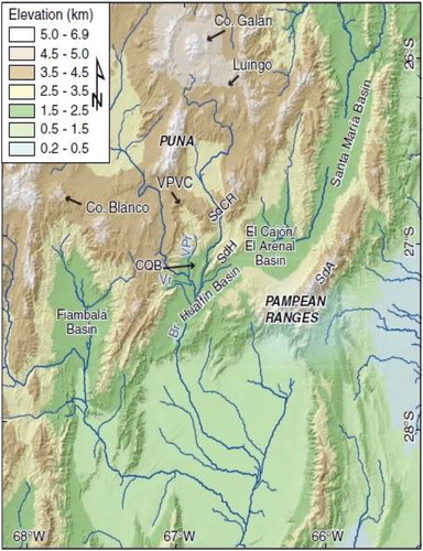
The study area is Cerro Blanco volcanic field between 26${}^{°}$′S to 26${}^{°}$54′S latitudes and 67${}^{°}$36′W to 67${}^{°}$54′W longitudes. Cerro Blanco is a caldera in the Catamarca Province in Argentina (Figure 2). Part of the Central Volcanic Zone of the Andes, it is a volcano collapse structure located at the altitude of 4400 m. The Central Volcanic Zone of the Andes is an area between 14${}^{°}$ and 28${}^{°}$ southern latitude. Cerro Blanco was the site of the largest-known Holocene eruption in the Central Andes about 5 ka (Fernandez-Turiel et al. 2013). The rhyolitic eruption produced plinian ash fall deposits of about 110 km³ and spread ignimbrite deposits across an extensive area. Its summit elevation is approximately 4400 m so it is a high volcano on which few studies have been completed thus far, for example, Brunori et al. (2013) and Báez et al. (2015). One of the principal characteristics of the Cerro Blanco which makes it unique among the actively deforming volcanoes is that it is subsiding (Pritchard and Simons, 2004) and (Henderson and Pritchard, 2013).

Figure 2. Regional morphology with superimposed river network derived from a 30-m resolution Shuttle Radar Topography Mission (SRTM) digital elevation model of Cerro Blanco in the North West of Argentina. Source: (Guzmán et al. 2017).

The data set used in this study includes multiple radar images acquired by the European Space Agency satellite ENVISAT. The data set contains 14 images in descending orbit (track 10) and spans the periods 2003–2007. Images are in VV polarization with an incidence angle of 23${}^{°}$ and azimuth of –168${}^{°}$. The processing chain in the StaMPS-MTI method (Hooper, 2008) was implemented. StaMPS-MTI allows exploiting two A-InSAR (Advanced InSAR) techniques; the permanent scatterers (PS) technique (Ferretti et al. 2001) and the small baseline subsets (SBAS) technique (Berardino et al. 2002).

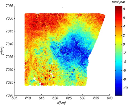
By combining these two approaches, a deformation signal for a greater number of points can be obtained. Besides, the deformation signal in the combined application of the two techniques has a higher overall signal-to-noise ratio than that of obtained via each single technique individually. When dealing with limited data set like the study here, combination of the two approaches leads to more reliable results. Mean velocity fields and the deformation history of the Cerro Blanco were calculated. The retrieved map shows a distribution of negative and quasi circular deformation pattern (movement away from the satellite in the line of sight (LOS)) as shown in Figure 3. The measured rate of subsidence has a maximum value of –12 mm/yr in the radar LOS (Brunori et al. 2013).

Figure 3. Surface velocity map, related to the time period April 2003 and January 2007 (ENVISAT data set), obtained by applying the A-InSAR method of StaMPS-MTI. Source: (Brunori et al. 2013). Coordinates are in UTM.

4. Simulated tests

Before the application of the inverse MFS on the Cerro Blanco volcano, the method is compared with the analytical spherical model in a test area in two separate cases for comparison. These two cases are with and without the topography effect, respectively. In the case, where the effect of topography is not considered, a 20 × 20 km area is considered as the external boundary $\partial \Omega$ (Figure 4). To obtain the amount of displacement on the outer boundary, the relationships presented in Mogi (1958) for a sphere magma source under the origin, at the depth of 5.5 km, the volume change of 0.01 km³, and the radius of 1 km in a homogeneous elastic half space was used. Equation (17) as the MFS of the half space was used. Poisson ratio for this problem is assumed 0.25 and a shear modulus of elasticity in accordance with geological studies in some volcanic areas was estimated at 7 GPa. The error added to the boundary values has normal distribution with variance of 0.5 cm². This variance is comparable to the real variance of InSAR data (Shirzaei and Walter, 2009). A total of 324 boundary points scattered uniformly on the outer border as well as 64 points on the unknown inner border were considered. The source points, parallel and outside the outer boundary and inside the inner boundary, are shown schematically in Figure 4. The inside points are located within a sphere under the origin with a radius of 0.3 km. The number of boundary and source points and the distance of the source points from the domain were selected such that increasing them will not cause a significant decrease in the RMSE value of the solution.

Figure 4. Coordinate system and the domain of the problem in the case of without topography effect which contains upper surface as the outer boundary $\partial \Omega$ and the unknown inner boundary D. The circles represent the boundary points and the squares represent the source points. They are distributed uniformly and the source points are parallel to the boundaries.

The initial value for the unknown coefficients equals zero (Karageorghis et al. 2011a) and for internal boundary a 3 D smooth star-shape with a maximum and minimum radius of 1.2 and 0.7 km (Beauducel et al. 2004) were assumed, respectively. The position of the magma source centre (C) as the unknown parameters was added to the problem. However, the regularization term ${\mu }_3\left|\mathbf{C}\right|$ is not included. In Karageorghis et al. (2016), there were only a small number of components and numerical solutions with no implications for the instability of C. Initial coordinates of the magma source centre were set as $X=$0.1, $Y=$0.1, and the depth as $Z=-$5.4 km. First, the problem was solved without considering the regularization parameters as shown in Figure 5(a). Consequently, the results of the model do not conform to a sphere shape as expected from a magma source. In the second stage, ${\mu }_1>0,{\mu }_2=0$ as suggested in Karageorghis et al. (2016) were considered. Using the L-curve method, the regularization parameter was selected. As shown in Figure 6(a), the optimal amount of μ₁ equals 10 ^{– 3}. The results are illustrated in Figure 5(b) and Table 1. The RMSE between the deformation fields of the modelled magma source and those of the analytical sphere is 0.5 cm. Table 1 shows the calculated position of magma source centre which shows a satisfactory agreement with the centre position of the Mogi model. In comparison with Figure 5(a) where no regularization was employed, it can be seen that the modelled magma source is closer to a sphere shape. Third, the problem was solved using ${\mu }_1=0,{\mu }_2>0$, again as suggested in Karageorghis et al. (2016).

Figure 5. Graphical representation of the results of modelling volcanic magma reservoir without considering topography effect (a) regardless regularization terms, (b) considering regularization term μ₁ and (c) considering regularization term μ₂. The sphere represents the analytical boundary and the dots represent the modelled boundary. All axes are in km.

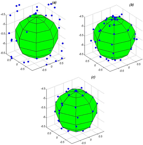
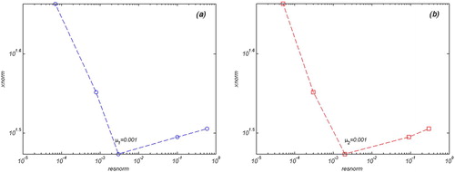
Figure 6. The L-Curves in the case of without topography affect (a) the L-Curve of the parameter μ₁, (b) the L-Curve of the parameter μ₂. In both figures, the horizontal axes show that the logarithmic scale of the residual norm and vertical axes is logarithmic scale of the solution norm.

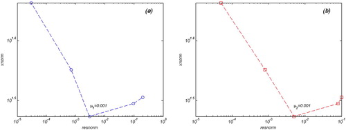
Table 1. Position of the centre of magma source.

Condition	X (km)	Y (km)	Depth (km)
Neglecting topography effect, considering ${\mu }_1>0,{\mu }_2=0$	$-0.002\pm 5\times {10}^{-6}$	$0.005\pm 3\times {10}^{-6}$	$-5.5\pm 2\times {10}^{-6}$
Neglecting topography effect, considering ${\mu }_1=0,{\mu }_2>0$	$0.001\pm 1\times {10}^{-6}$	$0.001\pm 2\times {10}^{-6}$	$-5.5\pm 1\times {10}^{-6}$
Considering topography effect, considering ${\mu }_1>0,{\mu }_2=0$	$-0.003\pm 4\times {10}^{-6}$	$0.004\pm 3\times {10}^{-6}$	$-8.3\pm 2\times {10}^{-6}$ (bs)
Considering topography effect, considering ${\mu }_1=0,{\mu }_2>0$	$0.001\pm 1\times {10}^{-6}$	$0.001\pm 1\times {10}^{-6}$	$-8.3\pm 1\times {10}^{-6}$ (bs)

Note: X, Y horizontal coordinates (in defined coordinate system), Depth = depth to source centre. bs is stand for below the summit.

The corresponding the L-curve with a corner value of ${\mu }_2={10}^{-3}$ is illustrated in Figure 6(b). The results of the third scenario are shown in Figure 5(c) and Table 1. The RMSE is 415$\times {10}^{-3}$ cm. Again in comparison with Figure 5(a,b) and Table 1, the shape of the magma source and its centre position is a more satisfactory fit to that of the analytical model. This shows further improvement. Considering the RMSE values, Figure 5(b,c), it is demonstrated herein that both these cases of the magma source modelling were completed with a satisfactory accuracy (i.e. the sphere shape of the magma source and its centre point coordinates). Evidently, in the model with the regularization state and ${\mu }_1=0,{\mu }_2={10}^{-3}$, the most accurate results have been achieved with a satisfactory conformation to the analytical magma source model.

To elaborate on the modelling in this study, the effect of topography is considered. The volcano edifice is a cone with the radius of 5 km, the average slope of the flank is $\alpha ={30}^{°}$ and the altitude of H = 2886 m. The cone data are added to the previous boundary as the topography (Figure 7). To calculate the displacements caused by a centre of dilatation as the outer boundary data set, the method of Williams and Wadge (1998) was used. The effect of topography is considered in this method. Various depths of magma source are also assumed at each point. Similar to the models where the effect of topography was not considered, the error added to the boundary values has normal distribution with a variance of 0.5 cm². Poisson ratio, shear modulus of elasticity and initial shape of magma source are similar to the previous models. 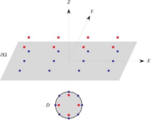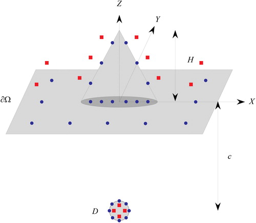Equations (15)(15) $$G_{ij}(P,Q)=\frac{1}{16\pi \mu (1-\nu )R}\left((3-4\nu ){\delta }_{ij}+R_{,i}{R}_{,j}\right)$$(15) and (17) were used as the MFS of topography and half space, respectively. On the topography surface, the boundary points were selected to form a uniform network. These points also map on the half space to form the boundary points of the medium. 64 points were distributed uniformly on the inner boundary. They totally constituted 440 points. The source points, outside the outer boundary and inside the inner boundary are located on a sphere under the origin with the radius of 0.3 km, as shown in Figure 7 schematically. According to Cayol and Cornet (1998), the depth of magma reservoir should be considered from the summit. Accordingly, the initial values for the position of the magma source centre are $X=$0.1, $Y=$0.1 and $Z=$−8.1 km. Other parameters are similar to those of the previous models. First, the problem was solved without considering the regularization parameters.

Figure 7. Schematic view of boundary and source points distribution. The circles represent boundary and the squares represent source points, respectively. The cone as a schematic topography has been shown. H is the height of summit and c is the magma source depth.

In Figure 8(a), the results of the solution regardless of the regularization term are given. The results do not conform to a sphere. In the second stage considering ${\mu }_1>0,{\mu }_2=0$, the problem was solved. Selecting the regularization parameter was done using the L-curve method and as shown in Figure 9(a), the optimal amount of equals 10^{– 3}.The results are illustrated in Figure 8(b) and Table 1. RMSE is 0.36 cm. In comparison with Figure 8(a) where no regularization was employed, the modelled magma source is closer match to a sphere. According to Table 1, the position of the magma source centre including its depth estimated herein is in a satisfactory agreement with that of the analytical model. Then, the problem was solved using ${\mu }_1=0,{\mu }_2>0$. Figure 9(b) represents the L-curve of this case which ${\mu }_2={10}^{-3}$ is the corner of the curve. The results are shown in Figure 8(c) and Table 1. RMSE is 227$\times {10}^{-3}$cm. Again in comparison with Figure 8(a,b) and Table 1, the form of the magma source and its centre position conform to the estimation of the analytical model.

Figure 8. Graphical representation of the results of modelling volcanic magma reservoir considering topography effect (a) regardless regularization terms, (b) considering regularization term μ₁ and (c) considering regularization term μ₂. The sphere represents the analytical boundary and the dots represent the modelled boundary. All axes are in km.

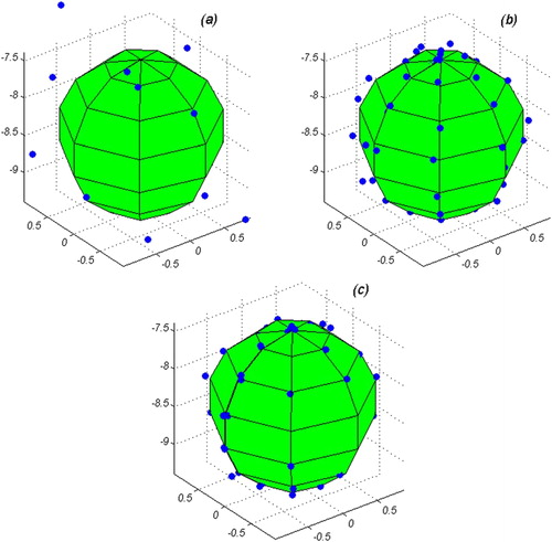
Figure 9. The L-Curves in the case of considering topography affect (a) the L-Curve of the parameter μ₁, (b) the L-Curve of the parameter μ₂. In both figures, the horizontal axes show that the logarithmic scale of the residual norm and vertical axes is logarithmic scale of the solution norm.

The results show further improvement. Considering the RMSE values, Figure 8(b,c) and Table 1, in both cases (i.e. second and third scenario), the geometry of the magma sources was simulated in a satisfactory agreement with those estimated via the analytical models. Nevertheless, at the regularization state where ${\mu }_1=0,{\mu }_2={10}^{-3}$, the most satisfactory agreement has been achieved. The modelling shows that in both cases irrespective of considering the effect of topography, the MFS is a robust method for modelling the magma source geometry.

5. Application of the inverse MFS on Cerro Blanco volcano

Cerro Blanco volcano is considered in this study as a case to perform the inverse MFS on. Similar to the simulated tests, the inverse MFS is executed in both cases of considering the effect of topography and otherwise. A system of Cartesian coordinates with the origin located at the mean sea level, just below Cerro Blanco summit, is assumed. In this case, x and y axes are orientated along WE and SN directions, respectively, while the z-axis points up out of the medium. The outer boundary has been defined to coincide with the data coverage used in this study. The initial value for the unknown coefficients was assumed zero similar to the previous simulations. The effect of topography is not considered at this stage. To determine the initial coordinates of the magma source centre, GA on the InSAR data for a spherical magma source was performed in a homogeneous elastic half space. X = 0.9, Y= −1.2 and $Z=-$9.5 km below mean sea level (bmsl) were selected. Initial magma source as a 3 D smooth star shape located at the selected position with maximum and minimum radius similar to the aforementioned simulations were considered. Poisson ratio like other volcanoes was assumed as 0.25 and shear modulus, similar to Ruch et al. (2009) study, was inputted at 20 GPa. For the boundary values of the outer boundary, InSAR measurements were used. Equation (17) as the MFS of the half space was applied. A total of 432 boundary points distributed uniformly on the outer boundary as well as 200 points on the unknown inner boundary was considered. The source points were distributed parallel and outside the outer boundary and inside the inner boundary on a sphere located under the origin with the radius of 0.3 km. On this basis, the problem was solved considering ${\mu }_1>0,{\mu }_2=0$ and ${\mu }_1=0,{\mu }_2>0$, respectively. Selection of the regularization parameter was done using the L-curve method. As shown in Figure 10(a,b) the optimal values of ${\mu }_1,{\mu }_2$ equal 10^{– 3}. The results are illustrated in Figure 11(a)–(d). The positions of the centre of magma source in both cases are illustrated in Table 2. RMSE between the deformation fields of the modelled magma source and InSAR observations for both cases are 0.62 and 0.5 cm, respectively. In order to investigate the effect of topography on modelling, a digital elevation model (DEM) provided by the shuttle radar topography mission (SRTM) was considered (Figure 12). An initial magma source as a 3 D smooth star shape located at the depth of 9.9 km from the summit was considered. The planar coordinates are $X=$0.9 and $Y=-$1.1, again at the range suggested in Henderson and Pritchard (2013). Equations (15)(15) $$G_{ij}(P,Q)=\frac{1}{16\pi \mu (1-\nu )R}\left((3-4\nu ){\delta }_{ij}+R_{,i}{R}_{,j}\right)$$(15) and (17) were used as the MFS of the topography and the half space, respectively. Other parameters are similar to the case where the effect of topography was not considered. On the topography surface, the boundary points were selected to form a uniform network. These topographical boundary points when projected on the half space form the boundary points of the latter medium. 200 points also uniformly were distributed on the inner boundary. They totally constituted 1064 points. MFS was implemented in the first case with the assumption of ${\mu }_1>0,{\mu }_2=0$ and at the second case for ${\mu }_1=0,{\mu }_2>0$. To determine, the L-curve method was used as shown in Figure 13. The values of these parameters were selected at the 10^{– 3}. These are the optimum values for regularization in both cases. The magma source was modelled and the results are presented in Figure 14 and Table 2. The RMSE is approximately 4 mm for the first case and circa 3 mm for the second case. According to Figure 14 and Table 2, the results of the MFS are in a satisfactory agreement to the analytical model in Henderson and Pritchard (2013) where a spherical source with a radius of 1 km with the centre of $X=$1 and $Y=-$1, and the depth of 10 km for the Cerro Blanco volcano was calculated. They used inversion of the InSAR data to model the magma source. From review of both scenarios where the effect of topography was and was not considered, the following conclusion can be drawn. If an inversion is performed on the observed surface displacements, the shape and the horizontal position of the magma chamber centre is almost similar in both scenarios. However, neglecting topography could cause the depth of the chamber to be overestimated. In the case of neglecting topography, the depth is calculated at 9.82 km below mean sea level whereas in the case of considering the effect of topography the depth was calculated at 9.999 km below the summit or 5.6 km below the mean sea level, confirming the findings of Williams and Wadge (1998).

Figure 10. The L-Curves in the case of without topography effect of Cerro Blanco (a) the L-Curve of the parameter μ₁, (b) the L-Curve of the parameter μ₂. In both figures, the horizontal axes show that the logarithmic scale of the residual norm and vertical axes is logarithmic scale of the solution norm.

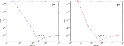
Figure 11. Results of modelling Cerro Blanco magma reservoir using inverse MFS without the effect of topography (a) side view considering μ₁, (b) top view considering μ₁, (c) side view considering μ₂ and (d) top view considering μ₂. Axes are in km.

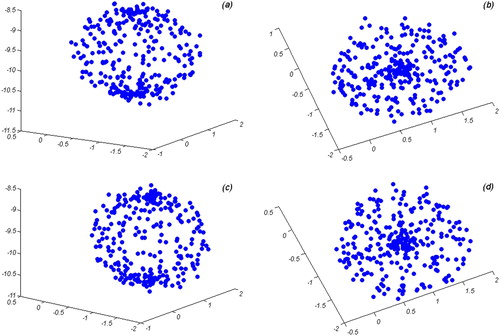
Figure 12. DEM of Cerro Blanco area that is completely covers Cerro Blanco volcano. Black star shows Cerro Blanco summit. Coordinates are in UTM.

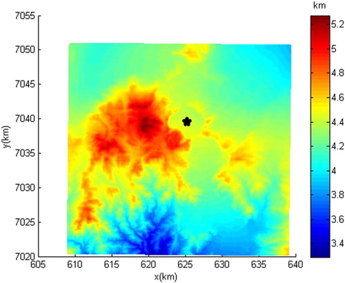
Figure 13. (a) The L-Curve of the parameter μ₁, (b) the L-Curve of the parameter μ₂. Axes are similar to simulated test.

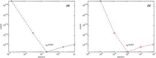
Figure 14. Results of modelling Cerro Blanco magma reservoir using MFS and considering the topography effect (a) side view considering μ₁, (b) top view considering μ₁, (c) side view considering μ₂ and (d) top view considering μ₂. In all figures, the sphere shows the suggested magma source model in previous study and the blue dots are the MFS results. Axes are in km.

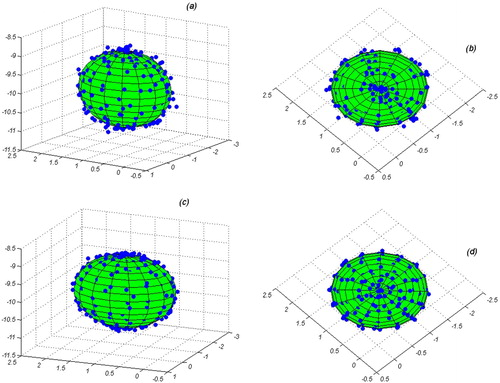
Table 2. Position of the centre of magma source in Cerro Blanco.

Condition	X (km)	Y (km)	Depth (km)
Neglecting topography effect, considering ${\mu }_1>0,{\mu }_2=0$	$0.9\pm 5\times {10}^{-6}$	$-0.7\pm 3\times {10}^{-6}$	$-9.8\pm 2\times {10}^{-6}$(bmsl)
Neglecting topography effect, considering ${\mu }_1=0,{\mu }_2>0$	$0.95\pm 3\times {10}^{-6}$	$-0.9\pm 2\times {10}^{-6}$	$-9.82\pm 1\times {10}^{-6}$(bmsl)
Considering topography effect, considering ${\mu }_1>0,{\mu }_2=0$	$1.002\pm 5\times {10}^{-6}$	$-1.002\pm 3\times {10}^{-6}$	$-9.98\pm 2\times {10}^{-6}$(bs)
Considering topography effect, considering ${\mu }_1=0,{\mu }_2>0$	$1.001\pm 4\times {10}^{-6}$	$-1.001\pm 1\times {10}^{-6}$	$-9.999\pm 1\times {10}^{-6}$(bs)
Henderson and Pritchard (2013)	1	–1	–10 (bs)

Note: X, Y = horizontal coordinates (in defined coordinate system), Depth = depth to source centre. bmsl and bs are stand for below mean sea level and below the summit, respectively.

6. Conclusions

In this study inverse 3 D MFS was used to determine the geometry of a volcanic magma source. It is a geometric inverse problem with linear elasticity characteristics. The study shows that the MFS is relatively easy to implement, does not require a lot of data preparation and unlike the BEM in which the singularities or source points are outside the domain, it does not face with the troublesome integrations. In the first instance, the method was conducted on the simulated area with and without considering the effect of topography. The numerical results show that when the input data has small error, the output is calculated with a large error and the problem is unstable. Regularization can be achieved either by appropriately limiting the number of functional evaluations or by introducing regularization in terms of the objective cost function which is to be minimized. In the current study, the second method using the Thikhonovs method and an L-curve regularization was employed. For both conditions of considering the effect of topography and otherwise, the three cases before regularization, ${\mu }_1>0,{\mu }_2=0$ and ${\mu }_1=0,{\mu }_2>0$ were investigated. The results show that in both conditions at the regularization state and considering ${\mu }_1=0,{\mu }_2>0$, the magma source geometry is in its best conformity to the analytical model. Then, the inverse MFS was performed on the Cerro Blanco volcano. The volcano is a high-altitude one barely investigated previously. To show the effect of topography on the results both cases of with and without the effect of topography were surveyed. For this purpose, the real topography was used. In the case of neglecting the topography, RMSE was estimated at 6 and 5 mm in two separate cases of regularizations. A sphere at the depth of 9.82 km below the mean sea level was modelled as the magma chamber in this case. In the second case where the effect of the topography was considered, the RMSE was calculated at approximately 4 and 3 mm, again in two respective cases of regularizations. A sphere at the depth of 5.6 km below the mean sea level or 9.999 km below the summit was modelled as the magma chamber in this latter case. This is consistent to the previous investigation on the volcano. The investigation herein shows that if an inversion was performed on the observed surface displacements, the shape and the horizontal position of the magma chamber centre is almost similar in both cases of considering and neglecting the effect of topography. Nevertheless, neglecting topography could cause the depth of the chamber to be overestimated. Due to the inverse MFS being a meshless method, the simplicity of using the method and its accuracy, it is concluded that the inverse MSF investigated and applied in this study proves a robust methods in modelling the magma cavity. The method has also been shown to have the capability to determine the volcanic deformation field, particularly in cases of dealing with a large data set.

Acknowledgements

Sar data have been provided by the European Space Agency. We would also like to thank Professor Carlo Alberto Brunori for providing the InSAR displacement data of the study area.

Disclosure statement

No potential conflict of interest was reported by the authors.

References

- Alves CJ, Martins NF. 2009. The direct method of fundamental solutions and the inverse kirsch-kress method for the reconstruction of elastic inclusions or cavities. J Integral Equ. Appl. 21(2):153–178.
- Aster RC, Borchers B, Thurber CH. 2011. Parameter estimation and inverse problems. Vol.90. Academic Press.
- Báez W, Arnosio M, Chiodi A, Ortiz-Yañes A, Viramonte JG, Bustos E, Giordano G, López JF. 2015. Estratigrafía y evolución del complejo volcánico cerro blanco, puna austral, argentina. Revista mexicana de ciencias geológicas. 32(1):29–49.
- Beauducel F, Natale G, Obrizzo F, Pingue F. 2004. 3-d modelling of campi flegrei ground deformations: role of caldera boundary discontinuities. Geodetic Geophysl Effects Associated Seismic Volcanic Hazards.1329–1344.
- Berardino P, Fornaro G, Lanari R, Sansosti E. 2002. A new algorithm for surface deformation monitoring based on small baseline differential SAR interferograms. IEEE Trans Geosci Remote Sens. 40(11):2375–2383.
- Bin-Mohsin B, Lesnic D. 2017. Reconstruction of a source domain from boundary measurements. Appl Math Model. 45925–939.
- Borman D, Ingham D, Johansson B, Lesnic D. 2009. The method of fundamental solutions for detection of cavities in eit. J Integral Equ. Appl. 21(3):381–404.
- Brunori CA, Bignami C, Stramondo S, Bustos E. 2013. 20 years of active deformation on volcano caldera: Joint analysis of InSAR and AInSAR techniques. Int J Appl Earth Observ Geoinformation. 23279–287.
- Camiz S, Poscolieri M, Roverato M. 2017. Geomorphometric comparative analysis of Latin-American volcanoes. J South Amer Earth Sci. 7647–62.
- Carbone D, Currenti G, Del Negro C. 2007. Elastic model for the gravity and elevation changes before the 2001 eruption of etna volcano. Bull Volcanol. 69(5):553–562.
- Carbone D, Currenti G, Del Negro C. 2008. Multiobjective genetic algorithm inversion of ground deformation and gravity changes spanning the 1981 eruption of Etna volcano. J Geophys Res: Solid Earth. 113(B7):
- Cayol V, Cornet FH. 1998. Effects of topography on the interpretation of the deformation field of prominent volcanoesapplication to Etna. Geophys Res Lett. 25(11):1979–1982.
- Delgado F, Pritchard M, Lohman R, Naranjo JA. 2014. The 2011 Hudson volcano eruption (southern Andes, Chile): Pre-eruptive inflation and hotspots observed with InSAR and thermal imagery. Bull Volcanol. 76(5):815.
- Fairweather G, Karageorghis A. 1998. The method of fundamental solutions for elliptic boundary value problems. Adv Comput Math. 9(1/2):69.
- Fernandez-Turiel J, Rodriguez-Gonzalez A, Saavedra J, Perez-Torrado F, Carracedo J, Osterrieth M, Carrizo J, Esteban G. 2013. The largest holocene eruption of the Central Andes found. In: AGU Fall Meeting Abstracts.
- Ferretti A, Prati C, Rocca F. 2001. Permanent scatterers in SAR interferometry. IEEE Trans Geosci Remote Sens. 39(1):8–20.
- Field L, Blundy J, Brooker R, Wright T, Yirgu G. 2012. Magma storage conditions beneath dabbahu volcano (Ethiopia) constrained by petrology, seismicity and satellite geodesy. Bull Volcanol. 74(5):981–1004.
- Golberg MA. 1995. The method of fundamental solutions for Poisson’s equation. Eng Anal Boundary Elem. 16(3):205–213.
- Guzmán S, Strecker MR, Martí J, Petrinovic IA, Schildgen TF, Grosse P, Montero-López C, Neri M, Carniel R, Hongn FD, et al. 2017. Construction and degradation of a broad volcanic massif: The vicuña pampa volcanic complex, southern Central Andes, NW Argentina. Bulletin. 129(5–6):750–766.
- Hansen PC. 1999. The l-curve and its use in the numerical treatment of inverse problems.
- Henderson S, Pritchard M. 2013. Decadal volcanic deformation in the Central Andes volcanic zone revealed by InSAR time series. Geochem Geophys Geosyst. 14(5):1358–1374.
- Hooper A. 2008. A multi-temporal InSAR method incorporating both persistent scatterer and small baseline approaches. Geophys Res Lett. 35(16):1-5.
- Karageorghis A, Lesnic D. 2009. Detection of cavities using the method of fundamental solutions. Inverse Probl Sci Eng. 17(6):803–820.
- Karageorghis A, Lesnic D, Marin L. 2011a. The MFS for the detection of inner boundaries in linear elasticity. Boundary Elem Other Mesh Reduct Methods. 33229–239.
- Karageorghis A, Lesnic D, Marin L. 2011. A survey of applications of the mfs to inverse problems. Inverse Problems in Science and Engineering. 19(3):309–336.
- Karageorghis A, Lesnic D, Marin L. 2013. A moving pseudo-boundary method of fundamental solutions for void detection. Numer Methods Partial Differential Eq. 29(3):935–960.
- Karageorghis A, Lesnic D, Marin L. 2016. The method of fundamental solutions for three-dimensional inverse geometric elasticity problems. Comput Struct. 16651–59.
- Latimer C, Samsonov S, Tiampo K, Manville V. 2010. Inverting for source parameters using a genetic algorithm applied to deformation signals observed at the Auckland volcanic field. Canad J Remote Sens. 36(sup2):S266–S273.
- Luzón F, Sánchez-Sesma FJ, Rodríguez-Zúñiga JL, Posadas AM, García JM, Martin J, Romacho MD, Navarro M. 1997. Diffraction of p, s and Rayleigh waves by three-dimensional topographies. Geophys J Int. 129(3):571–578.
- Marin L, Cipu C. 2017. Non-iterative regularized MFS solution of inverse boundary value problems in linear elasticity: A numerical study. Appl Math Comput. 293, 265–286.
- Mindlin RD. 1936. Force at a point in the interior of a semi-infinite solid. Physics. 7(5):195–202.
- Mogi K. 1958. Relations between the eruptions of various volcanoes and the deformations of the ground surfaces around them. Bull Earthquake Res Instit. 36:99–134.
- Mossaiby F, Ghaderian M, Rossi R. 2016. Implementation of a generalized exponential basis functions method for linear and non-linear problems. Int J Numer Methods Eng. 105(3):221–240.
- Nakao S, Morita Y, Yakiwara H, Oikawa J, Ueda H, Takahashi H, Ohta Y, Matsushima T, Iguchi M. 2013. Volume change of the magma reservoir relating to the 2011 Kirishima Shinmoe-dake eruptioncharging, discharging and recharging process inferred from GPS measurements. Earth. Planets Space. 65(6):3.
- Poullikkas A, Karageorghis A, Georgiou G. 2002. The method of fundamental solutions for three-dimensional elastostatics problems. Comput Struct. 80(3):365–370.
- Prezzi C, Risso C, Orgeira MJ, Nullo F, Sigismondi ME, Margonari L. 2017. Subsurface architecture of las bombas volcano circular structure (southern Mendoza, Argentina) from geophysical studies. J South Amer Earth Sci. 77:247–260.
- Pritchard M, Simons M. 2004. An INSAR-based survey of volcanic deformation in the Central Andes. Geochemistry, geophysics. Geosystems. 5(2):1–42.
- Riguzzi F, Atzori S, Obrizzo F, Pietrantonio G, Pingue F. 2012. Recent terrestrial and satellite observations to model deformations at Colli Albani volcano (central Italy). Int J Earth Sci (Geol Rundsch). 101(6):1661–1671.
- Rodríguez I, Roche O, Moune S, Aguilera F, Campos E, Pizarro M. 2015. Evolution of Irruputuncu volcano, Central Andes, northern Chile. J South Amer Earth Sci. 63385–399.
- Ruch J, Manconi A, Zeni G, Solaro G, Pepe A, Shirzaei M, Walter T, Lanari R. 2009. Stress transfer in the lazufre volcanic area, Central Andes. Geophys Res Lett.36(22):1–6.
- Saltogianni V, Stiros SC. 2013. A new algorithm for modelling simple and double Mogi magma sources in active volcanoes: Accuracy, sensitivity, limitations and implications. Bull Volcanol. 75(10):1–14.
- Shirzaei M, Walter T. 2009. Randomly iterated search and statistical competency as powerful inversion tools for deformation source modeling: Application to volcano interferometric synthetic aperture radar data. J Geophys Res: Solid Earth. 114(B10):1–16.
- Ulloa H, Iroumé A, Picco L, Mohr C, Mazzorana B, Lenzi M, Mao L. 2016. Spatial analysis of the impacts of the chaitén volcano eruption (Chile) in three fluvial systems. J South Amer Earth Sci. 69, 213–225.
- Williams CA, Wadge G. 1998. The effects of topography on magma chamber deformation models: Application to mt. Etna and radar interferometry. Geophys Res Lett. 25(10):1549–1552.