Estimation of flood land use/land cover mapping by regional modelling of flood hazard at sub-basin level case study: Marand basin

Abstract

Flood is one of the most dangerous environmental hazards that threaten the human lives and properties on a large scale. Identification of flood risk areas with the aim of optimal management of this area is very necessary. In this research, the estimation of Land use/Land cover (LULC) in the Marand basin was modelled on the Sub-basin level using remote sensing and geographic information systems (GIS). The runoff coefficient was determined using the LULC extracted from satellite images, slope map and soil hydrologic groups, and rainfall intensity. Then, peak runoff for each sub-basin was calculated. In the following, by using linear membership function in the fuzzy logic model, the integration of two layers of peak runoffs and the elevation line layers between 0 and 1 were transformed into fuzzy values. Afterward, by applying multiple overlaps of weights to each of these two layers and their results, classes of flood hazard distribution map were produced. By comparing the hazard map with the results of participatory geographic information system (PGIS) and entering this information into the confusing matrix, the collision accuracy of the map was 87.83%. Finally, by comparing this map with the land cover/use map, their flood extent was determined separately.

Keywords:

• Flood
• hazards
• fuzzy logic
• participatory geographic information system
• confusing matrix

Introduction

Flood is one of the main global hazards causing massive damages to industries such as agriculture, fisheries, housing, and infrastructures that heavily affects social and economic activities (Chang et al. 2008). It occurs after heavy rainfall due to rapid accumulation and the runoff from upstream to downstream. In studies of global hazards, flood is one of the main hazards that has affected the lives of people around the globe with many deaths (Borga et al. 2011). Flood accounts for about 40% of the deaths from natural hazards and only in the last decade, it has killed about 100,000 people and affected life of 1.4 billion people (Ezemonye and Emeribe 2011). Managing and reducing the flood hazard, play an essential role in maintaining the physical and social environment of different societies and their economic development (Huang et al. 2008). Also, managing this risk is crucial for reducing damage and adapting the effects of climate change to land use change. The purpose of risk here is the same probability of causing harm or expected damage resulting from interactions that occur in human or natural hazards and vulnerable situations (ISDR 2004). Therefore, the assessment and reduction of flood risks should not be ignored. The prediction of sudden flooding is complex and difficult and this risk is often associated with secondary incidents such as mass movements and soil erosion (Grimaldi et al. 2013). The Marand basin is in the East Azarbayjan province, which has been the source of many floods since the last years and has caused a lot of damages to different parts of the plantation, gardens, livestock, residential areas, and infrastructures including roads, bridges, and so on. According to a survey carried out at the Office of Protected and Engineering of Rivers and Beaches in the Regional Water Organization of East Azarbayjan Province (RWOEA), it has been determined that 51 flood events occurred in different areas of the Marand basin from 2003 to 2016. The recorded figures and results from the recent floods revealed that most of the flood-affected areas are mountainous and lacking hydrological statistics which explains an assessment of this area that is vulnerable to flood risk should be made in terms of flood hazard and Land use/Land cover (LULC).

From the past, remote sensing technology and geographic information systems (GIS) have been applied to assess and model flood risk at a widespread level globally (Van Westen et al. 2003; Althuwaynee et al. 2014). In this study, in order to determine the flood regions in Marand basin in the sub-basin scale, modelling was carried out in GIS environment. To have an accurate and up-to-date land use map, satellite images with 10 m spatial resolution were used and classified. By this map, along with the slope layer and the map of the hydrological group of the soil, the runoff coefficient of the basin was calculated. Also, using the rational model, the peak runoff in each sub-basin was calculated. After fuzzing the DEM layers and peak runoff, flood hazard index (FHI) was calculated by the overlapping factor. Finally, the area of the flood LULC was determined.

To get acquainted with the latest flood modelling and evaluation methods, many studies have been made on library and internet resources. Since, the Marand is one of the basins lacking hydrologic statistics. For this purpose, we should seek methods that use empirical methods to obtain citation estimates for flood hazard modelling. A sample of the worldwide studies has been presented as follows: (Asumadu-Sarkodie et al. 2015), in a research aimed at managing flood risk in Ghana using a modified rational model and rainfall data, it was finally determined that with increasing land, runoff coefficient, and peak runoff rates would increase. Franci et al. (2016) conducted a study in the Nicosia basin of Cyprus aimed at providing a flood risk map using simultaneously high-resolution spatial resolution and also using multivariate analysis on the five flood factors, and after calculation, the FHI of the study area was classified into seven classes. Vojtek and Vojteková (2016) published their study on flood hazard and flood risk assessment at the local spatial scale. In another research, Armenakis et al. (2017) investigated flood risk assessment in urban areas based on spatial analytics and social factors.

Study area and data

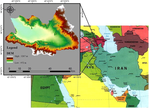
The Marand basin in the northwest of Iran with a geographical location 10˚45 to 10˚46˚ east and 15˚38 to 45˚38˚ north is located in the East Azarbayjan province. The area of this basin is about 2030 square kilometres. According to Iran’s Meteorological Organization, the average long-term rainfall in the region is about 395 mm and the average annual temperature in this region is 12.1° C. Its climate is Mediterranean with climatic features of semi-cold mountainous regions. The maximum and minimum altitudes of the area are 3267 and 972 metres respectively, and the average elevation is 1561 metres above free water level (Feizizadeh and Ghorbanzadeh 2017). The Marand Basin has four metropolitan areas and 183 villages with 245,000 inhabitants. The main economy of this region is based on agriculture and animal husbandry (East Azarbaijan Governorate, EAG 2017). Figure 1 shows the location of this area.

Figure 1 Case study area. Source: Author

LULC map

Since, the use of accurate LULC maps can improve the results of flood risk management (Bhatt et al. 2014). In this study, satellite images of Sentinel 2 A with a spatial resolution of 10, 20, and 60 m for different bands were used to generate the LULC map. Considering the frequency of flooding is in the months of August and May. The image posted on https://scihub.copernicus.eu in August. The classification of satellite images based on spectral information has some limitations, therefore, other information resources should be used to increase the accuracy of classification (Chen et al. 2009). In this research, the object-oriented classification method was used. Before performing its various stages, the image was visualized using the semi-automatic classification plugin (SCP) of the QGIS-corrected atmospheric image to eliminate the negative atmospheric effects in the image.

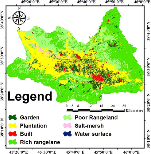
In addition to spectral information, texture and shape information is also used to enhance the classification accuracy in object-oriented image processing (OBIA) (Blaschke 2014). Because in this image processing method, based on the spectral, physical and geometric parameters of ground-based phenomena recorded on the image, segmented and image processing units from pixels to image phenomena or segments are changed, and as a result, by comprehensive processing of this information, objects and phenomena of the real world can be extracted more accurately. The process and the result of this type of image processing can be divided into three sections: segmentation, fuzzy classification, and validation (Aksoy and Ercanoglu 2012). For the segmentation in the eCognition software for the parameters of Scale Parameter, Shape, and Compactness, values of 50, 0.1, and 0.5 were considered respectively and AND and OR functions were used for fuzzy classification. The study area was divided into seven general classes in terms of LULC including garden, plantation, built, rich rangeland, poor rangeland, salt- marsh, and water surface. The Kappa coefficient and the overall accuracy of the map in the classification were 0.91 and 93.5, respectively, which is an acceptable accuracy. Figure 2 shows the map of the LULC classification of the study area.

Figure 2 Map of the LULC classification of the studied area. Source: Author

Soil texture map

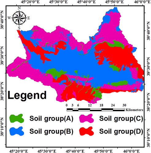
Soil properties affect the evolution of runoff and should be considered in its calculations. Soil properties can be expressed in terms of a hydrologic factor, which is the minimum permeability velocity in the long-term wet state of the crude. All soil textures are divided into four groups based on the Natural Resources Conservation Service (NRCS) indicators, each group can be divided into subgroups, if necessary, more accurately. The penetration intensity in soil hydrological groups and other characteristics of each group are presented (Council 1999). Thus in this study, the soil map was prepared using aggregation and analysis of soil texture reports and maps from RWOEA, natural resources organization (NRO), and agriculture research centre of East Azarbayjan (ARCEA), which is shown in Figure 3.

Figure 3 Map of soil hydrological groups of the studied area. Source: Author

Digital elevation model

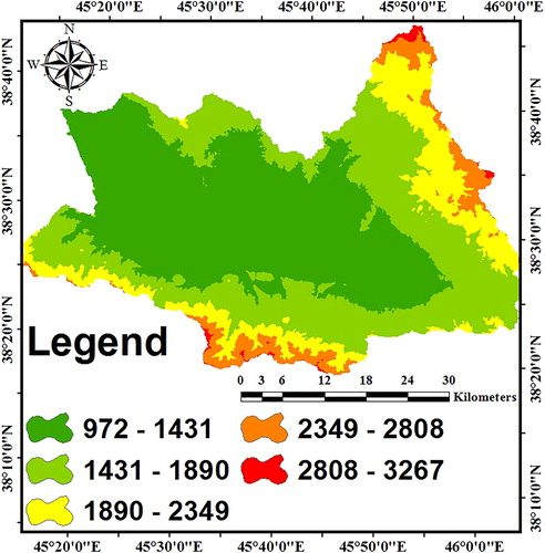
In flood risk assessment studies, using a digital elevation model of that area is very important in demonstrating the floodgates’ zones (Asare-Kyei et al. 2015). In this study, the digital elevation model (DEM) of the Aster TERRA satellite with a spatial resolution of 30 metres was used. According to Figure 4, the maps of the elevation classes in the study area are presented in five classes.

Figure 4 Map of the DEM classes. Source: Author

Slope map

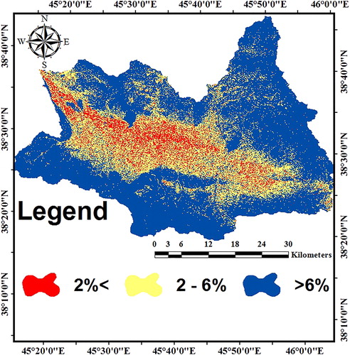
To provide a slope map in this research, the 30-metre digital elevation model Aster was used. Totally, the area is divided into low slopes in plain areas and harsh areas in mountainous areas. According to Figure 5, the map of the area is classified in three classes and is represented by percentage.

Figure 5 Slope. Source: Author

Rainfall intensity

In the northwest region of the country, up to 2400 metres high rainfall increases while after this height, the severity of these rainfall decreases, so that rainfall of more than 12 mm is rarely seen at those heights. (Motaleb Faed 2007). In the northwest region of Iran, there is a high correlation between the values ​of DEM and ground stations, and the physiographic factors of Sahand, Sabalan, and Misho heights affect the extreme rainfall (Valizadeh Kamran and Nasiri Qalehini 2013). In this research, in order to determine the intensity of rainfall for each sub-basin, the time of concentration of each sub-basin was determined based on kirpich method according to the Equation (1)(1) $$tc=0.0195{\mathrm{L}}^{077}{\mathrm{S}}^{-0.385}$$(1) . (1) $$tc=0.0195{\mathrm{L}}^{077}{\mathrm{S}}^{-0.385}$$(1)

In this equation;

tc = Concentration time of the basin in terms of hours

L = Length of the main waterway in km

H = Difference in height between the highest and lowest points of the basin (Wijesinghe and Wijesekera 2011). The length of the main waterway is also determined by the Equation (2)(2) $$L=1.312\mathrm{*}{A}^{0.568}$$(2) . (2) $$L=1.312\mathrm{*}{A}^{0.568}$$(2)

In this equation;

L = Length of the main waterway in km

A = Area in km² (Tribhuvan and Sonar 2016).

Based on the calculated values, it was found that the time for concentrating sub-basins was about 1 hour. In the following, the data of recorded logistic data with a period of 11 years including 2004 to 2015 at regional stations including the cities of Jolfa, Marand, Varzaghan, and Shabestar the same period rainfall events extraction were recorded from the intensity curves of the recorded rainfall.

Due to the inappropriate geographic distribution of precipitation stations, especially in mountainous regions, algebraic interpolation method was used based on DEM values according to the results of researches on northwest rangelands in Iran. According to Table 1, the maximum rainfall intensity of 1 hour, along with the geographic location and elevation of stations were prepared for conducting algebraic interpolation operations.

Table 1. Maximum rainfall intensity of 1 hour.

Longitude	Latitude	Elevation(m)	Max rainfall intensity(mm)	Station name
45.61	38.93	712	13.24	Jolfa
45.76	38.41	1375	12.54	Marand
46.63	38.5	1675	19.45	Varzaghan
45.7	38.16	1440	12.44	Shabestar

To determine the relationship between rainfall and DEM, linear regression was used in Excel software and the relationship (Garcia 2016) was determined according to Equation (3)(3) $$\mathrm{P}=0.004*\mathrm{m}+9.997$$(3) . (3) $$\mathrm{P}=0.004*\mathrm{m}+9.997$$(3)

The result of this equation shows that in this area, with an increase in height, also rainfall increases.

Methods

The studies have shown that there are a total of four main techniques for producing a flood hazard map. These techniques include hydrological frequency analysis, hydraulic modelling, hydrological models, and a statistical method (El morjani 2011). In this research, the combination of hydrological model and statistical method using the remote sensing and GIS, was used to generate a flood hazard map at the study area.

Integration of the hydrological and statistical model in GIS

To prepare the mapping of flood hazard areas with high spatial resolution in the sub-basin, it is necessary to combine the results of the two methods. Firstly, using the modified version of the hydrological model (Viessman and Lewis 1996), the amount of runoff is determined based on the intensity of rainfall, land use, and runoff coefficient of the basin. Then, the statistical method in the GIS environment is combined with the output of the hydrologic model, which is integrated with topography factors (DEM) to determine the severity of flood hazard in the study area. Finally, by defining the class for classification on the map of the risk of flood intensity, the FHI for flood risk areas is determined (Asare-Kyei et al. 2015).

Determination the peak runoff using rational model

This method is usually used in small basins and it is assumed that the rain is constant at all levels of the basin. The simple application of this method has led to widespread use in related studies, especially for urban hydrology and basin management. In this study, this model was used to calculate maximum runoff discharge, which is presented in accordance with the Equation (4)(4) $$\text{Qp}=0.28*\mathrm{C}*\mathrm{I}*\mathrm{A}$$(4) . (4) $$\text{Qp}=0.28*\mathrm{C}*\mathrm{I}*\mathrm{A}$$(4)

In this equation, Qp is the rate of peak runoff according to cubic meter per second, C, is the runoff coefficient derived from an empirically pre-designed table and each of them are prepared based on the slope of the area, the type of land use, as well as the hydrological group Soil of the region, I, is the rain intensity in millimetres per hour, and A, is the area of drainage area in square kilometres (Needhidasan and Nallanathel 2013).

Determination of surface runoff coefficient

Surface runoff coefficient is the ratio of rainfall height that flows on the ground surface and depends on factors such as intensity of soil permeability, the density of LULC, rainfall intensity, and slope. According to Table 2, the runoff coefficient of different regions determined by overlapping each of these factors (County 2008).

Table 2. Runoff coefficients determination.

	Soil Group A			Soil Group B			Soil Group C			Soil Group D
LULC	Slope (percent)			Slope (percent)			Slope (percent)			Slope (percent)
	<2%	%6-2	%6<	<2%<	%6-2	%6<	<2%	%6-2	%6<	<2%	%6-2	%6<
Built surface	0.65	0.67	0.69	0.66	0.68	0.70	0.68	0.70	0.72	0.69	0.72	0.75
Plantation	0.14	0.18	0.22	0.16	0.21	0.28	0.2	0.25	0.34	0.24	0.29	0.41
Garden	0.08	0.11	0.14	0.1	0.14	0.18	0.12	0.16	0.2	0.15	0.2	0.25
Poor Rangeland & Salt-mersh	0.15	0.25	0.37	0.23	0.34	0.45	0.30	0.42	0.52	0.37	0.50	0.62
Rich Rangeland	0.14	0.22	0.30	0.2	0.28	0.37	0.26	0.35	0.44	0.30	0.40	0.50

Flood statistical modelling

A peak runoff map is combined with the DEM layer to prepare a flood hazard plan. However, it is necessary to be standardized before combining two informative layers of peak and height runoff into their units such as cubic metres per kilometre for peak runoff and metres for elevation. Using the theory of fuzzy theories, before the combination of layers, standardization is performed on comparable scales (Malczewski 1999). The standardization of these layers was done using the fuzzy membership function in Arc/GIS software. Regarding the direct and linear relationship between peak runoff and flood probability, using linear membership function, the peak runoff layer was re-classified between upper and lower thresholds. This means that the lowest amount of runoff is the zero-value peak, meaning no membership or low-flood probability, while the highest amount of peak runoff is the one-value meaning full membership or the highest probability of flood is given. Other peak runoff values are between zero and one degree. This is a reversal to the DEM layer because low-altitude areas are likely to be higher, but high altitude areas are less likely to occur in flood events. Therefore, low and high altitude areas determined with one and zero degrees of membership, respectively (Asare-Kyei et al. 2015).

Distribution mapping of flood hazard preparation

To map flood hazard severity at different heights, standardized layers of height and peak runoff are combined with linear weight composition method (Malczewski 2000). This was done using the FHI equation in the Arc/GIS and by specifying the weight of each layer. The total weight of all layers should be equal to 1. In this study, each layer of DEM and runoff peaks rated 0.5. Equation 5(5) $$FHI={\sum }_{i=1}^{n}0.5\left(\text{DEM}\right)+0.5\left(\text{PEAK RUNOFF}\right)\mathrm{}\mathrm{O}\mathrm{R}\mathrm{}FHI=\mathrm{}{\sum }_{i=1}^n\mathit{\text{WiXi}}$$(5) is the flood risk index equation: (5) $$FHI={\sum }_{i=1}^{n}0.5\left(\text{DEM}\right)+0.5\left(\text{PEAK RUNOFF}\right)\mathrm{}\mathrm{O}\mathrm{R}\mathrm{}FHI=\mathrm{}{\sum }_{i=1}^n\mathit{\text{WiXi}}$$(5)

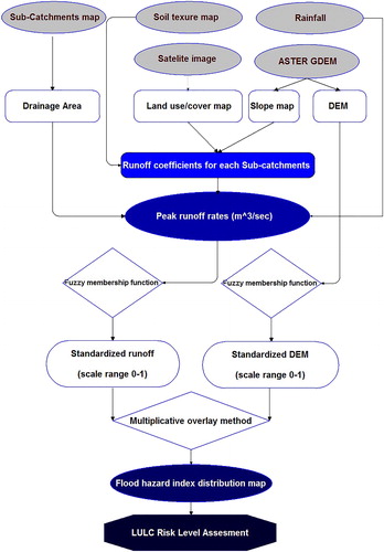
In the above equation, each parameter redescribed as follow: FHI, Xi, i-th standardized layer, Wi, the weight of each i-th layer and n is the number of combined standard layers. Since the weight of the standard layers is between zero and one, the value of the output pixels of the flood risk map is also within this range. Then, to identify areas with high and low risk of flooding, classification occurs in Arc/GIS environment. In this study, statistical methods were used in two stages. In the first step, standard statistical methods were used to obtain an FHI. In the second stage, statistical methods were combined using the principles of PGIS to assess the outcome of flood maps (Asare-Kyei et al. 2015). In the first step, using the rational model, the value of each of the factors affecting the peak flood flow was calculated. These effective factors include LULC, soil texture, slope map, DEM, and drainage area (El morjani 2011). Then, using statistical methods, runoff rates at different DEMs were determined before using standard methods for determining the flood hazard areas (Asare-Kyei et al. 2015). Figure 6 shows the flowchart of the research.

Figure 6 LULC risk level assessment flowchart.

Results and discussion

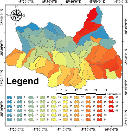
To determine the sub-basins, the Aster DEM and the Arc Hyrdo tools were used in 58 sub-basins. Figure 7 shows the distribution map of sub-basins.

Figure 7 Map of the case study sub-basins. Source: Author

Runoff coefficient calculation

Calculation of the runoff coefficient was done in two main stages, including the preparation of layers and then applying the multiplication overlap of these layers using GIS modelling. In order to accurately overlap the layers, data layer of LULC and soil texture map became rasterized, and then, along with a slope map, the pixel size of all of them adjusted at 10 × 10. In the following, using the Boolean logic (0 and 1), each of the classes in this map is also separated from each other. Using this logic, the class is worth one and the remaining unclassified classes are marked with zero value. This means that in this research, seven Boolean maps for LULC map, four Boolean maps for soil texture map and three Bolin maps were also provided for the slope map.

To overlap the different layers to calculate the runoff coefficient of the basin, all produced maps derived from the application of Boolean logic entered the GIS. Considering that according to Table 2 it is determined that each pixel with three characteristics of the slope, the type of application and the specified hydrological group, what is the runoff coefficient, and also many states are defined for determining these coefficients, the GIS modelling was used to perform this calculation. After multiplying the defined states in their specified coefficient, for all states in the table, at each pixel, the runoff coefficient was calculated and the output was taken. Finally, by applying the aggregation of all produced outputs, the runoff coefficient of the whole basin was prepared as shown in Figure 8.

Figure 8 The area runoff coefficient map. Source: Author

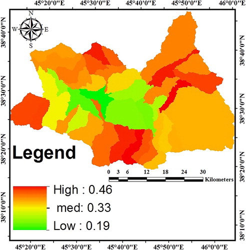
To determine the runoff coefficient of sub-basins separately and in terms of average in GIS, the average runoff coefficient for each sub-basin was calculated and the values of each sub-basin are shown in Figure 9.

Figure 9 Runoff coefficient of each sub-basin. Source: Author

To determine the peak runoff from rainfall intensity of 1 hour on each sub-basin, using the rational model, runoff coefficient layers, rainfall intensity, and area of each sub-basin were multiplied. The runoff rate for each sub-basin is given in Table 3.

Table 3. The peak runoff.

Sub-basin	Runoff (m^3/s)	Sub-basin	Runoff (m^3/s)	Sub-basin	Runoff (m^3/s)
1	67.01	21	55.55	41	76.26
2	89.1	22	58.82	42	35.61
3	53.61	23	49.59	43	37.48
4	91.1	24	23.95	44	27.82
5	68.95	25	35.18	45	71.19
6	41.21	26	53.30	46	85.12
7	56.64	27	47.60	47	68.3
8	47.96	28	12.45	48	98.36
9	51.35	29	101.15	49	18.43
10	100.03	30	62.16	50	26.38
11	89.36	31	42.71	51	62.97
12	21.77	32	82.89	52	31.93
13	56.18	33	42.27	53	69.18
14	68.78	34	53.49	54	27.89
15	43.39	35	42.93	55	43.78
16	80.20	36	121.07	56	66.6
17	36.97	37	56.86	57	69.92
18	76.31	38	45.23	58	71.47
19	18.86	39	102.44
20	42.17	40	101.52

Considering the correlation between runoff and DEM, the integration has been done using linear membership function of fuzzy logic model and peak runoff values as well as DEM distributed with phasing out between zero and one.

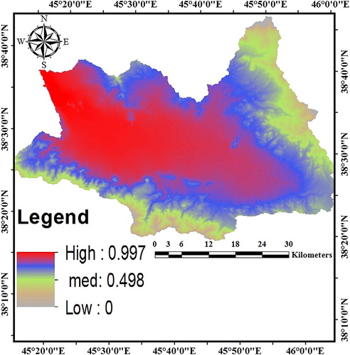
In the case of DEM layer, the lower the height, the more flooding occurs and the high DEMs are not flooded; therefore, in the fuzzy membership function, the low and high DEM regions are set to 1 and zero, respectively. Figure 10 shows the fuzzy map of the DEM layer between zero and 1.

Figure 10 The fuzzy map of DEM. Source: Author

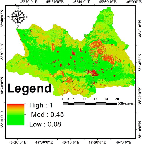
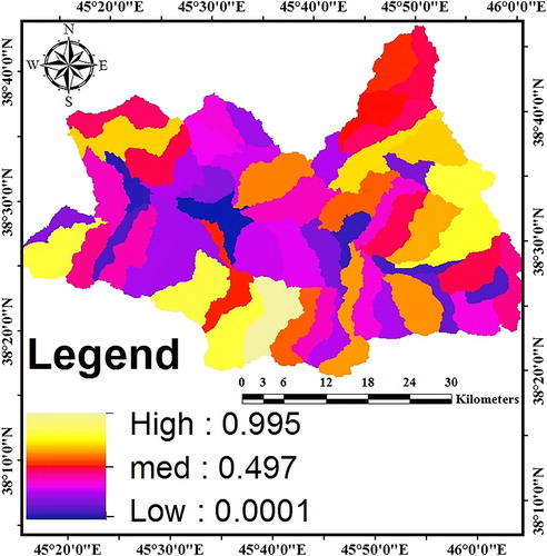
In the case of peak runoff, this is upside down, the higher peak runoff, the greater the flooding, and vice versa, the lower the peak runoff, the lower this rate, therefore, in the fusion membership function, the higher peak runoff, tends to number 1 and the less runoff tends to zero. Figure 11 shows the fuzzy map of peak runoff from 1 hour rainfall intensity between zero and 1.

Figure 11 The fuzzy map of peak runoff. Source: Author

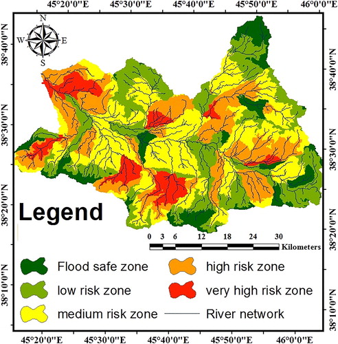
To generate a flood hazard intensity map at different DEMs, height standardized and peak runoff layers were combined using linear weight composition method. This procedure was completed using the FHI equation in the GIS with specification the weight of each layer. Since, the total weight of all layers should be equal to one and there is a direct relationship between runoff and DEM, in this study, the weight of 0.5 was given to each one of DEM and peak runoff layers in the maximum rainfall intensity of 1 hour. Finally, the runoff layers and the fuzzy DEM of the area were multiplied by the coefficient and gathered together. After classifying the prepared map in five categories, the area with sub-basin levels divided into very high-risk, high-risk, moderate, low-risk, and very low-risk classes. Figure 12 shows a flood risk map with 1 hour rainfall intensity.

Figure 12 Flood hazard map. Source: Author

Verification of produced map

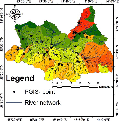
In this study, the PGIS was used to validate the final maps of Marand’s flood risk to determine the accuracy of the modelling performed. In this type of verification, local experts and authorities, using the science, experience, and historical memory of the floods occurred in different regions, as well as the natural characteristics of each sub-basin, determine the risk class of each region (Craig et al. 2002). In the present study, with the cooperation of experts with a high level of work in Marand County and native area water administrations who have proper knowledge of the area, flood, and hazardous levels in the area, a field survey was conducted to determine the accuracy of the produced maps. In the field survey, the risk class was marked with a GPS device according to Figure 13.

Figure 13 Map of the marked points with GPS devise. Source: Author

Comparison of the recorded points using PGIS and the risk maps obtained using the confusion matrix is presented, and this matrix is illustrated in Table 4.

Table 4. Confusion matrix estimating the accuracy of hazard maps.

Risk classes	Very high	High	Medium	Low	Safe	Total	Accuracy (%)
Very high	10	0	0	0	0	10	100
High	0	19	5	0	0	24	79.16
Medium	0	0	12	3	0	15	80
Low	0	0	0	4	1	5	80
Safe	0	0	0	0	5	5	100
total	10	19	17	5	5	59	87.83

According to the validation results of each classifications and the average of each five classes, it was found that the accuracy of the maps was 87.83%.

The purpose of this study was to assess the regional risk of flooding in the Marand basin in the Sub-basin level. In this study, using Sentinel 2A satellite imagery with a spatial resolution of 10 metres, the LULC types of the study area were carefully prepared. Since it is obvious that in order to obtain the higher accuracy of basin runoff factor, the higher precision of the image, as well as the prepared map of the soil hydrologic groups and the map of the used slope, the closer results are to the reality. By isolating each of the abovementioned classified maps using Boolean logic, all layers entered GIS modelling and using the runoff coefficient given in the table, the runoff coefficient of each sub-basin was determined and finally, peak runoff for each sub-basin was calculated with 1 hour rainfall intensity at sub-basin level. Then, using the linear membership function in the fuzzy logic model, the DEM and peak runoff amounts were fuzzy. Also, by applying the multiplication of assigned weights for each of these layers according to the FHI, the final flood risk map of the study area was determined in five risk classes including very low-risk, low-risk, moderate, high-risk, and very high-risk. By comparing the results of the designated classes and the values recorded in field observations using the GPS device, the provided confusion matrix showed the accuracy of produced maps as 87.83%. In order to determine the flooding of each LULC, the flood hazard map was compared with the LULC map and according to Table 5, the risk level of each cover/use class was separately determined.

Table 5. Area of each LULC in flood risk classes.

LULC	Very high	High	Medium	Low	Safe
Garden	10.85	38.65	55.5	45.16	13.02
Plantetion	58.92	153.8	200.63	104.36	23.51
Built surface	2.92	14.32	20.58	11.41	2.03
Water surface	0.06	0.25	0.39	0.078	0
Rich rangeland	49.55	136.46	239.11	289.52	142.44
Poor rangeland	53.55	127.89	123.33	84.51	11.4
Salt-mersh	1.32	4.44	6.12	3.9	0.02
Total	177.17	475.81	645.66	538.94	192.42

In the investigation and comparison of risk categories in the occurrence of Marand basin flood, with considering the high-risk and very high-risk classes, which subsequently cause the most damages to different types of LULC, it was found that the class of rich rangeland with consisting of 186.01 km², it is exposed to the most vulnerable conditions. The area of LULC categories affected by flood risk is presented in Table 6.

Table 6. Area of high and very high risk categories of LULC.

LULC	Garden	Plantation	Built	Rich Rangeland	Poor Rangeland	Salt -mersh
Area(km^2)	49.5	74.3	17.3	186.01	181.44	5.76

The area of all classified materials is significant in flood hazard, so that totally 25.3% of the entire LULC area is in high and very high risk categories. Constructed lands including urban, rural, industrial, and industrial-productive centres, with a significant area of about 17.3 square kilometres, is at risk of flooding and vulnerability. Garden and plantation with a surface area of 123.8 square kilometres are at the risk of flooding as one of the most important sources of indigenous income. Every year they are heavily affected by the flood damages, especially their local economy. Also, poor and rich rangeland, which on the one hand, play an important role in terms of penetration of atmospheric depression and soil erosion control in the region, and on the other hand, it is a suitable rangeland for the livestock of the region native people, are at the risk of flooding and vulnerability. The salt-mersh areas are subject to flooding and leaching. In addition to the salinization of runoff and soil, gradual entry into underground water prevents their proper use. The results obtained in this research can be used to prioritize sub-basins with the aim of proper management of flood hazard underwater basins. Recognizing the high risk areas will increase the productivity of the costs and reduce the mortal and financial losses.

Conclusions

In this study, using the modelling of empirical estimation of peak runoff, the regional flood risk of each LULC in Marand basin has been evaluated. The study area was divided into five risk classes. By comparing maps of the flood hazard areas and LULC and their adaptation to the results of PGIS, high and high risk areas were identified. The use of empirical modelling and provision of its precise required data can greatly increase the accuracy of the region flooding. Utilization of native and regional managers’ views can be highly effective to confirm the results of such research. It also seems that the efficiency of the current model and other models in this field, in areas without hydrologic statistics and with different climates, can correctly aim to determine the flood zones.

Disclosure statement

No potential conflict of interest was reported by the authors.

References

- Aksoy B, Ercanoglu M. 2012. Landslide identification and classification by object-based image analysis and fuzzy logic: an example from the Azdavay region (Kastamonu, Turkey). Comput Geosci. 38(1):87–98.
- Althuwaynee OF, Pradhan B, Park HJ, Lee JH. 2014. A novel ensemble bivariate statistical evidential belief function with knowledge-based analytical hierarchy process and multivariate statistical logistic regression for landslide susceptibility mapping. Catena. 114:21–36.
- Armenakis C, Du EX, Natesan S, Persad RA, Zhang Y. 2017. Flood risk assessment in urban areas based on spatial analytics and social factors. Geosciences. 7(4):123.
- Asare-Kyei D, Forkuor G, Venus V. 2015. Modeling flood hazard zones at the sub-district level with the rational model integrated with GIS and remote sensing approaches. Water. 7:3531–3564.
- Asumadu-Sarkodie S, Owusu PA, Jayaweera MPC. 2015. Flood risk management in Ghana: A case study in Accra. Adv Appl Sci Res. 6(4):196–201.
- Bhatt GD, Sinha K, Deka PK, Kumar A. 2014. Flood hazard and risk assessment in Chamoli District, Uttarakhand using satellite remote sensing and GIS techniques. Int J Innovat Res Sci Eng Tech. 3(8):15348–15356.
- Blaschke T, Hay GJ, Kelly M, Lang S, Hofmann P, Addink E, Queiroz Feitosa R, van der Meer F, van der Werff H, van Coillie F, et al. 2014. Geographic object-based image analysis–towards a new paradigm. ISPRS J Photogramm Remote Sens. 87:180–191.
- Borga M, Anagnostou EN, Blöschl G, Creutin JD. 2011. Flash flood forecasting, warning and risk management: the HYDRATE project. Environ Sci Pol. 14(7):834–844.
- Chang LF, Lin CH, Su MD. 2008. Application of geographic weighted regression to establish flood-damage functions reflecting spatial variation. Water SA. 34(2):209–216.
- Chen M, Su W, Li L, Zhang C, Yue A, Li H. 2009. Comparison of pixel-based and object-oriented knowledge-based classification methods using SPOT5 imagery. WSEAS Trans Inf Sci Appl. 3(6):477–489.
- Council AR. 1999. Guidelines for stormwater runoff modelling in the Auckland Region. Auckland Regional Council Technical Publication No, 108. http://www.aucklandcity.govt.nz/council/documents/technicalpublications/TP108%20Part%20A.pdf.
- County K. 2008. Knox County Tennessee stormwater management manual. Knoxville (TN): Knox County.
- Craig WJ, Harris TM, Weiner D, editors. 2002. Community participation and geographical information systems. In Community participation and geographical information systems. Boca Raton, Florida: CRC Press; p. 29–42.
- East Azarbaijan Governorate (EAG). 2017. East Azarbayjan Governorate. [accessed 2017 Oct]. http://ostanas.gov.ir/Page/83/%D8%B4%D9%87%D8%B1%D8%B3%D8%AA%D8%A7%D9%86-%D9%85%D8%B1%D9%86%D8%AF.html/.
- El Morjani ZEA. 2011. Methodology document for the WHO e-atlas of disaster risk. Exposure to Natural Hazards Version, 2.
- Ezemonye MN, Emeribe CN. 2011. Flood characteristics and management adaptations in parts of the Imo river system. Ethiop J Environ Studies Manage. 4(3):56–64.
- Feizizadeh B, Ghorbanzadeh O. 2017. GIS-based interval pairwise comparison matrices as a novel approach for optimizing an analytical hierarchy process and multiple criteria weighting. GI_Forum. 1:27–35.
- Franci F, Bitelli G, Mandanici E, Hadjimitsis D, Agapiou A. 2016. Satellite remote sensing and GIS-based multi-criteria analysis for flood hazard mapping. Nat Hazards. 83(S1):31–51.
- Garcia IM. 2016. Interpolation functions. [accessed 2016 Apr 6]. personales.gestion.unican.es/martinji/Interpolation.htm/.
- Grimaldi S, Petroselli A, Arcangeletti E, Nardi F. 2013. Flood mapping in ungauged basins using fully continuous hydrologic–hydraulic modeling. J Hydrol. 487:39–47.
- Huang X, Tan H, Zhou J, Yang T, Benjamin A, Wen SW, Li S, Liu A, Li X, Fen S, et al. 2008. Flood hazard in Hunan province of China: an economic loss analysis. Nat Hazards. 47(1):65–73.
- International Strategy for Disaster Reduction (ISDR) 2004. Living with risk: a global review of disaster reduction initiatives. New York (NY); Geneva (Switzerland): United Nations.
- Malczewski J. 1999. GIS and multicriteria decision analysis. New York: John Wiley & Sons.
- Malczewski J. 2000. On the use of weighted linear combination method in GIS: common and best practice approaches. Trans GIS. 4(1):5–22.
- Motaleb Faed R. 2007. Modeling the spatial distribution of lightning and thunder storms using satellite images in the northwest of the country [Master thesis]. Tabriz (Iran): Department of Natural Geography, Tabriz University.
- Needhidasan S, Nallanathel M. 2013. Design of storm water drains by rational method–an approach to storm water management for environmental protection. Int J Eng Technol. 5(4):3203–3214.
- Tribhuvan PR, Sonar MA. 2016. Morphometric analysis of a Phulambri river drainage basin (Gp8 Watershed), Aurangabad district (Maharashtra) using geographical information system. Int J Adv Remote Sens GIS. 5(1):1813.
- Valizadeh Kamran K, Nasiri Qalehini S. 2013. Investigation of Thunderstorm Rainfall in the Highlands of the Northwest of Iran, Report for the First National Conference on Geography, Urban Development and Sustainable Development, Tehran, Iran.
- Van Westen CJ, Rengers N, Soeters R. 2003. Use of geomorphological information in indirect landslide susceptibility assessment. Nat Hazards. 30(3):399–419.
- Viessman WJ, Lewis GL. 1996. Introduction to hydrology. New York (NY): Harper Collins College Publishers.
- Vojtek M, Vojteková J. 2016. Flood hazard and flood risk assessment at the local spatial scale: a case study. Geomat Nat Hazards Risk. 7(6):1973–1992.
- Wijesinghe WMD, Wijesekera NTS. 2011. Comparison of rational formula alternatives for streamflow generation for small ungauged catchments. Eng J Inst Eng Sri Lanka. 44(4):29.