Application of unmanned aircraft system (UAS) for monitoring bank erosion along river corridors

Abstract

Excessive streambank erosion is a significant source of fine sediments and associated nutrients in many river systems as well as poses risk to infrastructure. Geomorphic change detection using high-resolution topographic data is a useful method for monitoring the extent of bank erosion along river corridors. Recent advances in an unmanned aircraft system (UAS) and structure from motion (SfM) photogrammetry techniques allow acquisition of high-resolution topographic data, which are the methods used in this study. To evaluate the effectiveness of UAS-based photogrammetry for monitoring bank erosion, a fixed-wing UAS was deployed to survey 20 km of river corridors in central Vermont, in the northeastern United States multiple times over a two-year period. Digital elevation models (DEMs) and DEMs of difference allowed quantification of volumetric changes along selected portions of the survey area where notable erosion occurred. Results showed that UAS was capable of collecting high-quality topographic data at fine resolutions even along vegetated river corridors provided that the surveys were conducted in early spring, after snowmelt but prior to summer vegetation growth. Longer term estimates of streambank movements using the UAS showed good comparison to previously collected airborne lidar surveys and allowed reliable quantification of significant geomorphic changes along rivers.

Keywords:

• Unmanned aircraft system (UAS)
• photogrammetry
• streambank erosion
• rivers

1. Introduction

Estimates of geomorphic change along river corridors guide watershed and surface water management strategies. Streambank erosion can represent a large portion of overall sediment and nutrient (e.g. phosphorus) loading to river systems (Bauer et al. 2002; Walling et al. 2008; Langendoen et al. 2012; Foucher et al. 2017) and is therefore important to quantify as part of comprehensive catchment water quality studies. Measurement of bank erosion and channel change is also critical in understanding the geomorphic condition of river systems (Piégay et al. 2005; Kline and Cahoon 2010). Additionally, bank erosion monitoring informs assessment of risk to infrastructure and stream habitat posed by fluvial erosion (Kline and Dolan 2008; Thakur et al. 2012).

Several methods are available for measuring and monitoring streambank erosion and retreat. Traditional methods for direct measurement include cross-sectional surveys and bank pins (Lawler 1993; Lawler et al. 1999). Lidar (laser scanning) from both airborne and terrestrial platforms has resulted in more comprehensive and detailed measurement of bank movement (Thoma et al. 2005; Resop and Hession 2010; O’Neal and Pizzuto 2011; Grove et al. 2013) and hillslope and gully erosion (Perroy et al. 2010; Tseng et al. 2013; Pirasteh and Li 2017; Cavalli et al. 2017). Longer term (multiple years or decades) estimates of streambank erosion rates have been successfully made using combined airborne lidar and historical aerial photos (Rhoades et al. 2009; De Rose and Basher 2011; Garvey 2012) and by applying digital photogrammetry to historical imagery (Bakker and Lane 2017).

A common approach for quantifying geomorphological change involves the creation of digital elevation models (DEMs) from sequential surveys and then subtracting the later DEM from the earlier DEM; the resulting difference represents land elevation change between the two survey dates. The dataset derived from the differencing of sequential DEMs is often referred to as a DEM of Difference (DoD). This approach has been employed with survey data collected using photogrammetry, airborne lidar, and terrestrial laser scanning (Milan et al. 2007; Perroy et al. 2010; O’Neal and Pizzuto 2011; Bremer and Sass 2012; Tseng et al. 2013; Grove et al. 2013; Cavalli et al. 2017). Recent advances in the development of digital photogrammetry methods and unmanned aircraft system (UAS) platforms have resulted in a resurgence of photogrammetry being used to generate topographic data and DEMs to detect geomorphic change (Westoby et al. 2012; Miřijovský and Langhammer 2015; Eltner et al. 2017; James et al. 2017; Cook 2017).

Advancements in UAS technology, also known as unmanned aerial vehicles (UAVs) or drones, have given rise to a flexible and affordable system for collecting topographic data. UAS-based surveying can overcome some of the existing data collection shortcomings of ground surveys and manned aircraft systems, such as being limited to specific sites, high costs or the requirement of longer data collection lead-times. While DEMs and contours from aerial photography using photogrammetric methods have been available for decades, recent advances in image processing software, driven in part by innovations in computer vision and structure from motion (SfM) and multi-view stereo photogrammetric algorithms, have rapidly advanced the resolution of UAS topographic data. In contrast to historical photogrammetry surveying, UAV SfM photogrammetry typically uses only basic camera technology and an automated processing workflow resulting in far lower costs (Westoby et al. 2012; Carbonneau and Dietrich 2017). SfM is ideally suited for processing photos with a high degree of overlap taken from a wide variety of positions (i.e. a moving sensor) (Westoby et al. 2012). Originally developed by the computer vision field during the 1990s, SfM and variations have become widely available in desktop software packages such as Agisoft PhotoScan, Pix4D, and Microsoft Photosynth. Digital photogrammetric methods such as SfM are applicable to imagery collected using any platform, including handheld smartphone cameras (Micheletti et al. 2015), but have been more widely adopted to process imagery collected using UAS (Hugenholtz et al. 2013).

UAS-based photogrammetric surveying has seen many applications in recent years; reviews by Colomina and Molina (2014), Watts et al. (2012), and Whitehead et al. (2014) highlight UAS characteristics and applications in photogrammetry and remote sensing. Fluvial study applications include mapping bathymetry (Lejot et al. 2007), channel topography (Woodget et al. 2015; Tamminga, Hugenholtz, et al. 2015; Miřijovský et al. 2015) and production of very high resolution DEMs (Whitehead and Hugenholtz 2014; Micheletti et al. 2015; Neugirg et al. 2016). In addition, UAS-derived data have shown potential in quantifying bank erosion and monitoring volumetric change in fluvial settings due to flooding (Miřijovský et al. 2015; Miřijovský and Langhammer 2015; Tamminga, Eaton, et al. 2015; Cook 2017; Hamshaw et al. 2017). However, to date, UAS investigations of river channels have utilized surveys over a single river reach (i.e. short sections less than a kilometre in length) typically with multi-copter UAS. In addition, applications of UAS for geomorphic change detection along rivers have been limited to areas largely clear of obstructing vegetation. There remains need for evaluation of UAS-based photogrammetry applied over longer sections of river corridor encompassing more varied areas, particularly those with dense vegetation.

In this study, we apply UAS-based photogrammetry to monitor long (∼20 km) lengths of river corridors and quantify streambank erosion rates along multiple rivers in the northeastern United States. Bank erosion is calculated for select sites to illustrate the system performance. In addition, we discuss some limitations of UAS and recommendations for its application in a watershed management setting.

2. Methods

2.1. Study area

Data were collected along four rivers (Shepard Brook, Mad River, Winooski River, and New Haven River) located in central Vermont (Figure 1). This area of Vermont drains the western portion of the Green Mountain Range and is part of the Lake Champlain basin. The study area features a humid continental climate with mean annual precipitation of 40–60 mm (PRISM Climate Group 2015). Soils range from fine sandy loams derived from glacial till deposits in the uplands to silty loams derived from glacial lacustrine deposits in the lowlands (Underwood 2004; Fitzgerald and Godfrey 2008). Streambanks in the study area on average are approximately 2 m high, ranging from 1.3 to 3.8 m high (Hamshaw et al. 2017). Vegetation is highly varied and ranges from bare soils to tall grass/brush and tree cover (Hamshaw et al. 2017).

Figure 1. Map of study area and portions of river corridor surveyed with UAS. Source: Author

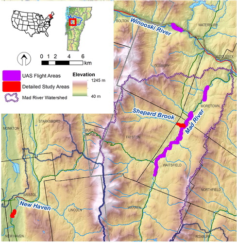
All four rivers have a significant history of flooding and resulting channel erosion that dates back to early settlements along the river corridor when historical deforestation of the watershed resulted in river channel destabilization (Underwood 2004; Fitzgerald and Godfrey 2008). During the last two decades, multiple flood events in each of the catchments have resulted in significant river channel erosion causing damage to infrastructure and impacts to water quality. The northeastern United States is experiencing increase in magnitude and frequency of rainfall events, a trend expected to continue (Betts 2012) making the study regionally relevant. Similar changes in weather are predicted elsewhere in the world. As rivers in such regions continue to adjust to a changing hydrological regime, data collected using UAS methods to monitor the current state of the river and its geomorphology are useful for broader watershed studies. Affordable methods such as UAS could prove very useful in tracking streambank erosion when UAS surveys can be collected every few years.

2.2. Data collection

UAS surveys took place during a two-year period between spring 2015 and spring 2017. The greatest number of flights were performed in spring months (April–May) when vegetation growth is at a minimum in Vermont and snow has melted. Additional survey campaigns were conducted along portions of the study rivers during summer (August) and late autumn (November–December). Topographic data obtained from airborne laser scanning (ALS) surveys were also used to calculate longer term amounts of erosion along portions of the New Haven River and Shepard Brook. ALS surveys were collected in May 2014 along the Mad River and Shepard Brook and in November 2012 for the New Haven River. The 2014 ALS survey was collected at an average point spacing of 0.7 m and the 2012 ALS survey at 1.6 m spacing.

During the study period, a few large storm events resulted in high river flows and caused channel erosion. These include an early spring rainfall event on 26 February 2015, which caused significant bank erosion along the New Haven River; and a mid-summer flash flood event on 17 August 2016 caused moderate bank erosion along Shepard Brook. Additionally, a number of large river flows occurred in the New Haven River in between the 2012 ALS survey and the 2015 UAS survey, which resulted in assumed periodic bank erosion. However, between the 2014 ALS survey and 2015 UAS surveys performed along the Mad River and Shepard Brook, no major storm events occurred; and therefore, streambank erosion was assumed to be minor.

UAS surveys were performed using a senseFly eBee fixed-wing UAS equipped with an RGB true-colour camera (Figure 2(a)). Three models of eBee were used over the study time period; the spring 2015 flights used the original eBee model, while subsequent campaigns utilized the eBee RTK or eBee Plus model (Table 1). The RTK and Plus models distinguish themselves from the standard model by incorporating a survey-grade, real-time kinematic (RTK) GPS receiver to directly georeference the data with sub-metre accuracy as well as the higher resolution RGB cameras. For UAS data collected with the standard eBee model, ground control points (GCPs) were used to georeference the data. All UAS flights were collected with a target ground sample distance (GSD) of 3.6 cm with a resulting typical altitude above ground level of approximately 100 m. Lateral and longitudinal image overlap were both set to 70%. During the spring and late autumn survey campaigns, UAS flights occurred during ‘leaf-off’ conditions to help minimize the effects of vegetation.

Figure 2. (a) senseFly eBee UAS; (b) section of streambank along Shepard Brook in November 2015; (c) example of eroding streambank along Mad River in July 2015 with presence of summer vegetation growth; and (d) section of streambank along New Haven River that experienced significant erosion in April 2016. Source: Author

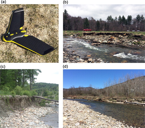
Table 1. UAS and their specifications used in survey campaigns.

UAS Model	Survey campaigns	Camera model	Weight	Wingspan
eBee	Spring 2015	Canon S110 (12 MP)	0.69 kg	96 cm
eBee RTK	Summer/Fall 2015, Spring/Summer 2016	Sony WX (18.2 MP)	0.7 kg	96 cm
eBee Plus	Spring 2017	senseFly S.O.D.A. (20 MP)	1.1 kg	110 cm

2.3. DEM analysis

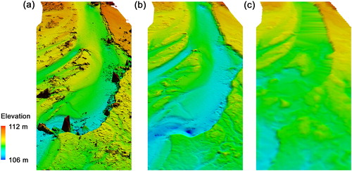
The UAS imagery were first post-processed using senseFly’s eMotion Version 3.3.4 software and then passed through the Pix4D Version 4.0.21 (Pix4D, Inc.) software package for photogrammetric processing. Like other digital photogrammetric UAS solutions, the Pix4D processing has a seamless workflow that ingests UAS imagery, generates a three-dimensional point cloud from the overlapping images, and uses the point cloud to produce an orthorectified image mosaic and raster digital surface model. Pix4D also has the capability to automatically generate a DEM (Figure 3(b)), also referred to as a digital terrain model (DTM), from the DSM (Figure 3(a)) and point cloud using a proprietary, machine learning-based algorithm. The UAS-based DEMs had a cell size of 0.15 m compared to 1.0 m and 0.7 cm for the 2012 ALS and 2014 ALS surveys, respectively. We note that various methods and software packages are available that enable generation of DSMs and DEMs from point cloud data. We used the automated DEM generation provided by the senseFly and Pix4D system, as it is representative of an automated and efficient workflow for generating topographic data over large areas and multiple survey campaigns.

Figure 3. Three-dimensional perspective view of a portion of the New Haven River as seen in (a) DSM from April 27, 2016 UAS Survey, (b) DEM generated from April 27, 2016 UAS survey, and (c) DEM from 2012 ALS survey. Source: Author

The DEM accuracies were evaluated using GCPs collected along selected river reaches. The GCPs were surveyed using a TopCon HiperLite + differential GNSS (Global Navigation Satellite System) receiver. The GCP positions were collected with the GNSS rover in a semi-kinematic (‘stop‐and‐go’) mode; and the GNSS base station positions were corrected using the Online Position User Service (OPUS) provided by the National Geodetic Survey of the National Oceanic and Atmospheric Administration. DEMs from the airborne lidar surveys (Figure 3(c)) utilized in this study were publicly available from the State of Vermont and are considered a hydro-flattened DEM.

To compare DEMs generated from multiple survey dates, DEMs of difference (DoDs) were generated in Quick Terrain Modeler Version 8.0.4 (Applied Imagery). The DoDs were calculated between successive UAS surveys as well as between UAS DEMs and the ALS DEM. DoDs were consistently calculated by subtracting the later date survey from the earlier date; thus, resulting negative values indicate erosion.

2.4. Streambank erosion calculation

During the study period, one particular portion of the New Haven River experienced significant channel movement and bank erosion (horizontal bank movement >10 m). This river reach is at high risk for channel erosion and has been subjected to previous river channel stabilization efforts (Underwood 2004; Underwood et al. 2014). Other portions of the Shepard Brook, Mad River, and Winooski River study areas had localized areas of minor to moderate erosion (horizontal bank retreats ∼ 1 m). In this paper, we highlight analysis of channel change and measurement of streambank erosion along two river reaches: a 1.2 km section of the New Haven River site with significant channel movement and a 1.5 km section of Shepard Brook with minor bank erosion (Figure 1).

The volumetric change of streambank erosion along the river corridor was calculated from the DoD models within a pre-defined river corridor area. The river corridor area was delineated to approximate areas subjected to river flows during a high water level or where potential bank erosion might occur. Both a total negative (erosion) and positive (aggradation) elevation change along the river corridor can be determined as well as a net change.

3. Results and discussion

3.1. Data acquisition and accuracy

Over the course of a two-year monitoring period, we conducted UAS surveys that covered nearly 50 km of river length. An overview of survey coverage and fieldwork effort is shown in Table 2. The greatest number of flights (55) were completed in 2015 where surveys were performed in early spring, mid-summer, and late autumn in contrast to 2016 and 2017 where surveys occurred primarily only in early spring. The average river length surveyed in a single flight was 553 m, although longer distances were achieved in the 2016 and 2017 surveys where average length of river per flight averaged 760 and 843 m, respectively. The greater efficiency during the later flights was likely due to a few factors including better optimization of flight lines, fewer equipment issues, and for the 2017 surveys, the greater battery capacity of the eBee Plus UAS.

Table 2. Summary of 2015–2017 UAS flights and survey coverage.

Year	Number of flights	Total length of river surveyed (km)	Mean length of river per flight (m)	Total days^a in field for surveying	Number of days impacted^b by weather
2015	55	21.7	395	12	3
2016	18	13.7	760	5	5
2017	17	14.3	843	4	1

^aA field day was considered 8 hours in the field, with approximately 6 hours available for survey efforts given 2 hours for travel accommodation.

^bImpacted survey days refer to those that were either cancelled and rescheduled due to rain or wind or those days cut short due to wind or rain.

The river corridor surveys required a total of 21 full-days in the field to collect. With a total of 49.7 km of river corridor surveyed, the average length per day was 2.37 km collected in approximately four flights (average of 4.3/field day). Rainy and excessively windy weather conditions resulted in rescheduling some field days or cutting them short. Out of 21 survey days, 9 (43%) required rescheduling or shortening. Difficulties with weather conditions varied from year-to-year. However, spring 2016 was especially challenging. All five survey days were in Spring (April and May) when rainfall is more frequent in the northeastern United States than other months, had to be rescheduled.

Comparison of the resulting DEM values to a set of GPS-surveyed GCPs at the two areas (Table 3) shows the mean errors were lowest for the ALS survey with −0.02 m for the New Haven River survey and 0.04 m for the Shepard Brook. UAS survey performance was highest with the April 2017 surveys. Errors for both ALS and UAS surveys were higher at the Shepard Brook site compared to the New Haven River area. Across all UAS surveys, we found an average median error of 0.09 m. This compares well to a previous study that found median vertical errors of 0.11 m in UAS-derived topographic data (Hamshaw et al. 2017).

Table 3. Assessment of accuracy of DEMs based on comparison to GCPs.

	2012 ALS	2015 UAS	2016 UAS	2017 UAS
New Haven River Site (n = 16)
Mean error (m)	0.02	0.25	0.12	0.04
Median error (m)	0.02	0.23	0.08	0.02
Standard deviation error (m)	0.09	0.09	0.15	0.12
RMSE (m)	0.09	0.26	0.19	0.12
Shepard Brook Site (n = 10)	2014 ALS	2017 UAS
Mean error (m)	0.04	−0.09
Median error (m)	0.00	0.03
Standard deviation error (m)	0.20	0.36
RMSE (m)	0.19	0.35

We found that using a sparse network of GCPs (i.e. 3-4 GCPs per survey area) was helpful to adjust for any overall bias/datum shift and as error check. The use of direct georeferenced topographic data in combination with a small number of GCPs has been found effective also by Carbonneau and Dietrich (2017).

3.2. Calculation of streambank erosion

3.2.1. Application to New Haven River

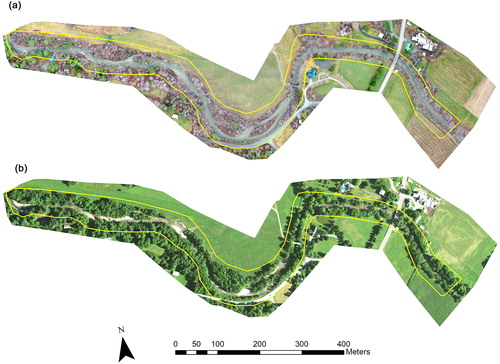
We surveyed a 1.2 km section of the New Haven River that experienced significant bank erosion and river channel movement during the study period. Between the November 2012 ALS survey and the December 2015 UAS survey, extensive channel movement was evident (Figure 4) as the result of a number of storm events. Continued erosion along portions of the streambank was apparent from subsequent UAS surveys in April 2016 and April 2017. A large amount of erosion was attributed to a February 2016 rain event that caused high river flows. All UAS surveys were completed during what would be considered ‘leaf-off’ conditions when vegetation growth was minimal and deciduous trees had dropped their leaves. During summer, the vegetation and tree cover along this section of the New Haven were fairly extensive (Figure 4(d)). The December 2015 UAS survey covered a smaller area than the 2016 and 2017 surveys due to flights being shortened by rainfall.

Figure 4. Section of the New Haven River as seen in (a) aerial imagery from April 2012, (b) UAS orthomosaic imagery from December 2015, (c) UAS orthomosaic imagery form April 2017, and (d) aerial imagery from July 2016. Area indicated by yellow boundary represents area of river corridor used in the analysis of DEMs. Source: Author

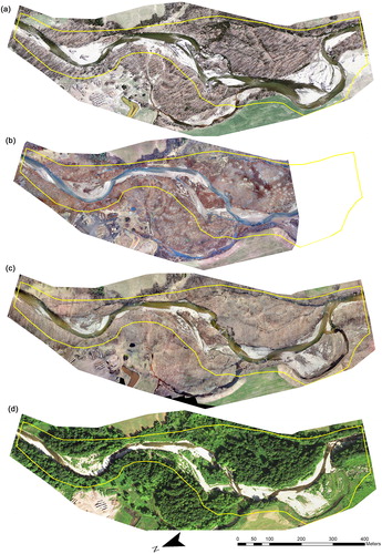
Automated DEM generation of the 2016 and 2017 UAS surveys produced high-quality topographic data with few obvious vegetation errors and little missing data (Figure 5). At the time of the spring UAS surveys, vegetation was noticeably less dense than during the December 2015 UAS survey. The presence of denser vegetation along areas of the river (dark brown areas of Figure 4(b)) during fall can be seen in the December 2015 UAS orthomosaic imagery. We observed, in spring, vegetation was matted down form snowpack resulting in greater visibility of the ground surface.

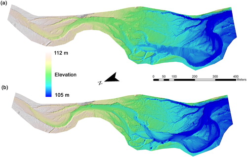
Figure 5. DEM of the New Haven River produced from (a) 2012 ALS survey and (b) 2017 UAS survey. Source: Author

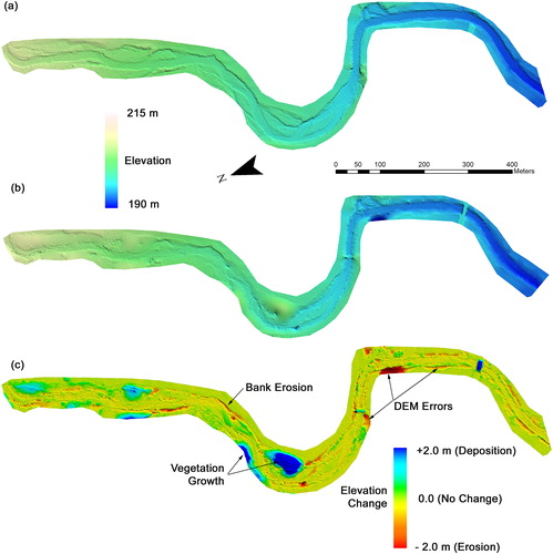
DoDs generated from multiple date DEMs allowed for spatio-temporal analysis of topographic change within the river corridor area. Between the April 2017 UAS and November ALS 2012 surveys, a net volumetric change of −19,920 m³ occurred over the 15.2 ha area. The changes included isolated areas of both deposition and erosion (Figure 6). In all, an estimated 31,509 m³ of erosion occurred and 11,589 m³ of deposition or aggradation was evident over the nearly five-year period. We also evaluated the geomorphic change at the intermediate survey date of April 2016, which confirmed the majority of erosion occurred between 2012 and 2016, compared to 2016 and 2017 (Table 4). Of note, the net change calculated between 2012 and 2016 was −14,056 m³ and −5,866 m³ from 2016 to 2017, giving a total net change of −19,922 m³, which is consistent with the net change calculated by differencing 2017 − 2012. The average annual rate of volumetric erosion was ∼6,300 m³/year. If an average bank height of 1.9 m (based on field measurements) is assumed over the entire 1,200 m long river reach, the average annual rate of bank retreat is estimated at 1.4 m/yr/m across each bank which equates to an average annual lateral migration of the river channel of 2.8 m/yr.

Figure 6. Elevation change between surveys along a section of the New Haven River as visualized by DEMs of difference (DoDs) between (a) 2012 ALS survey and 2016 UAS survey, (b) 2016 UAS survey and 2017 UAS survey, and (c) 2012 ALS survey and 2017 UAS survey. Source: Author

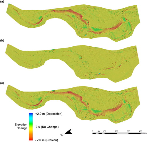
Table 4. Summary of volumetric change of surface within river corridor area for the New Haven River.

DoD model	Positive Change (Deposition) m^3	Negative Change (Erosion) m^3	Net Change m^3
2017 UAS – 2012 ALS	11,589	31,509	−19,920
2017 UAS – 2016 UAS	5503	11,369	−5866
2016 UAS – 2012 ALS	13,848	27,904	−14,056

We utilized the automated DTM (DEM) generation capability of Pix4D Mapper Version 4.0.5, which was released during the study period; the frequency of software releases highlights the rapid evolution of the UAS imagery processing and SfM photogrammetric techniques. With a number of proprietary algorithms packaged in various softwares, it is not unexpected that different software produces slightly different DEMs. While we did not study the impact of different software packages, Ouédraogo et al. (2014) found that DEM generation from two different software packages, Agisoft PhotoScan and MicMac, resulted in root-mean-square error (RMSE) difference of 4.9 cm. Vallet et al. (2012) found a similar scale difference (6.3 cm) in mean error between DTMs generated by Pix4D and the photogrammetric processing of SocetSet NGATE. These scale differences were minor relative to the scale of geomorphic change quantified in our study; and therefore, we do not believe the differences will impact our conclusions. Cook (2017) compared topography and volumetric changes derived using photogrammetric point clouds instead of DEMs with promising results. However, we elected a more conventional DEM analysis because of the readily compatible raster datasets and variety of analysis tools offered in common spatial analysis software packages such as ESRI ArcGIS.

Differences in water surface and vegetation growth were potential sources of additional error that we identified in the DEMs. Errors due to vegetation in the 2016 and 2017 UAS DEMs were not significant as evidenced by the small change in elevation observed in areas where significant vegetation growth can be observed during the summer. When comparing water surface elevations across a relatively stable portion of the river, we found differences of ∼0.2 m in the DEMs derived from the UAS and the ALS surveys. Negligible differences were observed between the 2016 and 2017 UAS surveys. While it is possible that river bed lowering occurred during the study period, we did not simultaneously measure bathymetry in the field; and given the reliability of SfM techniques for measuring bathymetry (Cook 2017), our analysis did not provide conclusive evidence of bathymetric changes. Studies have shown that bathymetric UAS measurements can be improved through refraction correction (Lejot et al. 2007; Dietrich 2017) to reduce errors.

The DEM quality from the December 2015 UAS survey was somewhat inferior in contrast to the April 2016 and 2017 surveys. Observation of the DoDs (Figure 7) revealed significant areas of measured deposition in places where no observed deposition occurred. In referring to the aerial imagery (Figure 4), these areas correspond to denser vegetation areas and show significant interpolation and smoothing in the DEMs. Errors in the 2015 DEM due to vegetation are also evident in the volumetric change between the 2017 and 2015 DoD (Figure 7(b)), which showed a net change of 1,401 m³ in areas where erosion was known to occur, and a negative net change was expected. The December 2015 UAS flight was also conducted in light rain conditions, which resulted in poorer image contrast compared to the spring 2016 and 2017 imagery. The greater density of vegetation in late autumn and possibly other factors made DoD calculations using the 2015 UAS survey less reliable. However, areas of significant erosion can be clearly identified in the dataset; and therefore, measuring erosion at specific individual areas would be required, compared to measurement over the entire river corridor area.

Figure 7. DoD for the New Haven River as calculated from (a) 2012 ALS survey and 2015 UAS survey and (b) 2015 UAS survey and 2017 UAS survey. Source: Author

3.2.2. Application to Shepard Brook

In contrast to the New Haven River area, Shepard Brook has different characteristics (i.e., denser vegetation and greater tree cover in the river corridor); it also is a smaller river with shorter streambanks (∼1.2 m high) and is less susceptible to channel movement and bank erosion. Between the May 2014 ALS survey and April 2017 UAS survey, several medium size storm events caused minor observable erosion in isolated locations. A short duration flash flood event in summer 2016 caused the greatest amount of bank erosion, but still only along short sections (e.g. site shown in Figure 8) and with less than 1 m of retreat over 3 years. Intermediate UAS surveys were completed in April 2015, August 2015, November 2015, May 2016, and August 2016. In analysing geomorphic change, we only compared in detail the April 2017 UAS survey to the 2015 ALS survey in order to compute the greatest amount of change when generating the DoD.

Figure 8. Section of the Shepard Brook as seen in (a) UAS orthomosaic imagery from April 2017 and (b) aerial imagery from July 2016. Area indicated by yellow boundary represents area of river corridor used in the analysis of DEMs. Source: Author

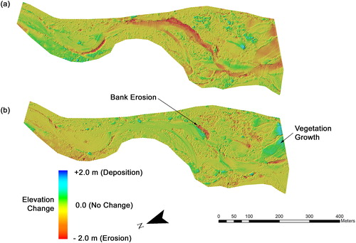
Errors in the UAS DEMs were more prevalent at the Shepard Brook site than the New Haven River site. Large areas of smoothed/interpolated data occurred in locations with thick tree cover where the UAS imagery could not reliably capture the ground surface (Figure 9). Similarly, missing data resulting from smoothing can be observed along much of the streambank. Shepard Brook has greater tree cover along the streambanks compared to the New Haven River, which may explain the poorer performance. This can be observed in the DoD generated between 2017 UAS and 2014 ALS survey (Figure 9(c)). The large areas of vegetation along the banks resulted in an over-estimation of erosion values along many portions of the river channel. This is also evident in the estimate of volumetric change over the river corridor, which showed a likely inaccurate net change of 13,372 m³, with respective estimates of total positive change (deposition) of 21,766 m³ and total negative change of 8,034 m³. However, some areas with active erosion (such as shown in Figure 9(b)) along portions of the river corridor reasonably clear of significant vegetation and tree cover were captured in the DoD (Figure 9(c)). In these individual areas, estimates of volumetric change were calculated more reliably due to the lack of noise caused by vegetation. For example, an ∼100 m length of eroding bank (identified in Figure 9(c)) had a net change −855 m³ between the 2017 UAS and 2014 ALS surveys when calculations were isolated to only that specific section of river. Based on visual field observations, this was the only area of active bank erosion along the stream reach during the study period, and therefore, the average annual bank erosion for the reach was 0.2 m/yr if an average bank height of 1.2 m was assumed over the entire 1.5 km reach.

Figure 9. DEMs of the Shepard Brook produced from (a) 2014 ALS survey and (b) 2017 UAS survey, and (c) DoD calculated from 2017 UAS survey – 2014 ALS survey. Source: Author

The results of DEM generation from Shepard Brook indicates that in densely vegetated river corridors, including those with a number of evergreen trees, a greater erosion threshold is necessary for UAS surveys to be reliable. Additionally, erosion estimates may be most successful when performed over specific smaller areas where DEMs are known to be more representative of the actual ground surface.

3.3. Comparison to existing studies of rates of bank erosion in the Lake Champlain Basin

The rates of channel movement and bank erosion from our study area were compared to previous studies of channel migration in the Lake Champlain basin. Jordan (2013) measured areas of channel migration along 13 main stem reaches of the Mad River between 1995 and 2011 using aerial imagery and found mean rates of lateral channel movement to range between 0.6 and 2.1 m/yr with an overall mean of 1.0 m/yr across all reaches. Another study estimated mean lateral channel migration along 10 Vermont rivers between 2004 and 2007 using a slightly different method by making use of aerial imagery and single airborne lidar survey and found mean lateral migrations between 0.2 and 0.5 m/yr with individual stream reaches as high as 0.8 m/yr (Garvey 2012; Ishee et al. 2015).

The 2.8 m/yr of channel migration we observed along the 1.2 km section of the New Haven River was greater than all the estimates found in previous bank erosion studies in the Lake Champlain basin. However, this result is certainly reasonable and likely represents the upper end of rates of expected channel movement in the region given the reach’s susceptibility to bank erosion due to its geologic setting and past upstream channel alterations (Underwood 2004) and that a large avulsion occurred during our study period. In contrast, the Shepard Brook reach, which had less extensive bank erosion (estimated lateral channel migration of 0.2 m/yr), is similar to the low-end of rates of channel movement observed in the other studies.

3.4. Characteristics of river corridors and relation to bank erosion estimates

The ability to detect geomorphic change in the river corridor using topographic data is a function of the magnitude of change, resolution of the topographic data, and the amount of error and noise in the data. We observed that the primary source of noise in the topographic data was due to the presence of heavy vegetation. Given that photogrammetric methods such as UAS-based SfM are line-of-sight survey methods that are dependent on being able to observe the surface of interest, the presence of noise in the data due to vegetation that obscures or partially obscures the data are expected. This is consistent with previous findings that dense vegetation can cause relatively large errors (Cook 2017; Hamshaw et al. 2017). As previously noted by Cook (2017), SfM techniques are capable of filtering out sparse vegetation effectively. We observed similar results at the New Haven River site, where spring UAS DEMs reliably captured the ground surface, filtering out the presence of sparse ground vegetation and trees. Therefore, we found that the usefulness of UAS-based photogrammetry for capturing streambank topography is informed more by the effective density of vegetation than the absolute presence.

The automated generation of DEMs in our study is surprisingly robust in filtering out the noise associated with sparse vegetation and trees. In climates similar to the northeastern United States, the timing of an UAS survey is critical as river corridors with deciduous tree cover and grass/brush are best surveyed in early spring after snowmelt but prior to summer vegetation growth. This is consistent with previous findings (Hamshaw et al. 2017) that assessed the capture of streambank topography using UAS and found early spring conditions had much lower errors than summer and autumn conditions. River corridors that feature year-round vegetation (i.e. tropical and subtropical climates) or the dominance of evergreen vegetation will offer limited opportunity for photogrammetric methods such as SfM.

3.5. Challenges and recommendations for UAS river corridor monitoring

This study utilizes the rapidly advancing technology of UAS and digital photogrammetry in surveying river corridors for the monitoring of streambank erosion. Many previous studies focused on acquisition and assessment of UAS-based topographic data along a single, relatively short river reach. In contrast, we collected survey data over ∼20 km of a varied set of river reaches. Studies seeking to evaluate geomorphic change are necessarily dependent on the timing of surveys to capture the land surface pre- and post-significant storm events. While our study areas were selected in part because of known occurrences of bank erosion and susceptibility to continued erosion, only very limited areas of significant bank erosion occurred as no large flood events occurred between survey dates. Therefore, while we have highlighted the application of UAS-based photogrammetry along two river sections, the quantification of UAS-based bank erosion along many river reaches needs further evaluation.

We also note differences in topography and land cover between our study area and many demonstrated applications of UAS for geomorphic change detection. In the northeastern United States, many river corridors are purposefully protected to preserve riparian vegetation and tree cover, which presents a challenge to remote sensing-based survey methods such as photogrammetry. However, given the flexibility in survey timing offered by UAS, we were able to wait for optimal survey conditions in order to acquire high quality topographic data along many river sections. In the process, we encountered several challenges in completing and processing data due in part to the use of an emerging technology, which in certain aspects is still in infancy, but at the same time rapidly advancing in some respects. We make the following recommendations as lessons learned for future UAS applications for surveying along river corridors including the application to geomorphic change detection and streambank erosion measurement.

1. For applications in continental and temperate climates, we recommend surveys be performed in spring conditions after snowmelt when vegetation is matted down and prior to ‘leaf-out’ to minimize errors caused by vegetation. Late-autumn conditions may also be appropriate provided there is not significant dead standing vegetation/brush still present.

2. The ability of the UAS-based photogrammetric method to capture the ground surface is dependent on the density of vegetation, not just the presence of vegetation. We recommend confirming, through site visits or from historical imagery, whether the area of interest, at any time of the year, is relatively free of dense, obscuring vegetation rather than relying on basic presence/absence of trees or vegetation noted in planning surveys.

3. For climates similar to the northeastern United States, we recommend anticipating the need to reschedule one-third of the planned survey days due to weather conditions. In our study, we found 43% of survey days were impacted by excessive wind or rain.

4. We found that an UAS with accurate, direct georeferencing capabilities, such as the eBee RTK and RTK-enabled eBee Plus, greatly simplified field data collection because they eliminated the need for GCPs. However, to achieve maximal accuracy or to accommodate a workflow utilizing lower cost UAVs, we recommend the collection of at least a sparse network of GCPs encompassing the entire survey area.

4. Conclusions and future work

The UAS application to monitor river corridors for streambank erosion presented here provides a cost-effective and efficient way to obtain high-resolution topography data on river corridors. While accuracy depended on the density of vegetation, we captured high-quality DEMs along river corridors with significant tree canopy and vegetation, provided surveys were conducted in early spring when optimal ground conditions occur. We utilized an automated workflow for georeferencing UAS-derived topography and generating DEMs that then allowed the direct comparison of multiple survey dates to airborne lidar surveys using a differencing of DEMs approach. The ability to calculate the volume of erosion and deposition along the entire river corridor provides a better understanding of the rate and pattern of bank erosion.

Given sufficient planning and selection of survey dates to achieve optimal vegetation and weather conditions, UAS-based photogrammetry provides topographic data that improve upon the resolution of currently available airborne lidar survey data. Given the ease of deploying UAS, surveying following large storm events to capture the topography of recently eroded areas offers a valuable tool for quantifying bank erosion. UAS technology is rapidly growing and new camera sensor technology, improvements in photogrammetric software and processing algorithms, and the direct georeferencing capability of GPS equipped UAVs should both improve the utility and performance of future systems.

Acknowledgements

The views, opinions, findings, and conclusions reflected in this paper are solely those of the authors and do not represent the official policy or position of any funding sources or endorse any third‐party products or services that may be included in this presentation or associated materials. The authors acknowledge the additional contributions of the University of Vermont (UVM) Spatial Analysis Lab UAS team and Kristen Underwood.

Disclosure statement

No potential conflict of interest was reported by the authors.

Additional information

Funding

This research was supported by the Vermont Water Resources and Lakes Studies Center. Additional support provided by Vermont EPSCoR with funds from the National Science Foundation (NSF) Grant EPS‐1101317 and OIA‐1556770, NSF Grant CMMI‐1229045, NSF Graduate Research Fellowship under Grant DGE‐0925179NSF, the Robert & Patricia Switzer Foundation, the Gund Institute for Environment, and Grant OASRTRS‐14‐H‐ UVM from the US Department of Transportation are also gratefully acknowledged.

References

- Bakker M, Lane SN. 2017. Archival photogrammetric analysis of river–floodplain systems using Structure from Motion (SfM) methods. Earth Surf Process Landforms. 42(8):1274–1286.
- Bauer DW, Mulla DJ, Sekely AC. 2002. Streambank slumping and its contribution to the phosphorus and suspended sediment loads of the Blue Earth River, Minnesota. J Soil Water Conserv. 57(5): 243–250.
- Betts AK. 2012. Historic trends and future climatic projections for Vermont. Presentation to the Vulnerability Assessment Workshop. Montpelier, Vermont.
- Bremer M, Sass O. 2012. Combining airborne and terrestrial laser scanning for quantifying erosion and deposition by a debris flow event. Geomorphology. 138(1):49–60.
- Carbonneau PE, Dietrich JT. 2017. Cost-effective non-metric photogrammetry from consumer-grade sUAS: implications for direct georeferencing of structure from motion photogrammetry. Earth Surf Process Landforms. 42(3):473–486.
- Cavalli M, Goldin B, Comiti F, Brardinoni F, Marchi L. 2017. Assessment of erosion and deposition in steep mountain basins by differencing sequential digital terrain models. Geomorphology. 291:4–16.
- Colomina I, Molina P. 2014. Unmanned aerial systems for photogrammetry and remote sensing: A review. ISPRS J Photogramm Remote Sens. 92:79–97.
- Cook KL. 2017. An evaluation of the effectiveness of low-cost UAVs and structure from motion for geomorphic change detection. Geomorphology. 278:195–208.
- De Rose RC, Basher LR. 2011. Measurement of river bank and cliff erosion from sequential LIDAR and historical aerial photography. Geomorphology. 126(1/2):132–147.
- Dietrich JT. 2017. Bathymetric Structure-from-Motion: extracting shallow stream bathymetry from multi-view stereo photogrammetry. Earth Surf Process Landforms. 42(2):355–364.
- Eltner A, Kaiser A, Abellan A, Schindewolf M. 2017. Time lapse structure from motion photogrammetry for continuous geomorphic monitoring. Earth Surf Process Landf 42(14):2240–2253.
- Fitzgerald EP, Godfrey LC. 2008. Upper mad river corridor plan. Waitsfield, VT: Friends of the Mad River.
- Foucher A, Salvador-Blanes S, Vandromme R, Cerdan O, Desmet M. 2017. Quantification of bank erosion in a drained agricultural lowland catchment. Hydrol Process. 31(6):1424–1437.
- Garvey KM. 2012. Quantifying erosion and deposition due to stream planform change using high spatial resolution digital orthophotography and Lidar data [M.S. Thesis]. Burlington, VT: University of Vermont.
- Grove JR, Croke J, Thompson C. 2013. Quantifying different riverbank erosion processes during an extreme flood event. Earth Surf Process Landf. 38:1393–1406.
- Hamshaw SD, Bryce T, Rizzo DM, O'Neil-Dunne J, Frolik J, Dewoolkar MM. 2017. Quantifying streambank movement and topography using unmanned aircraft system photogrammetry with comparison to terrestrial laser scanning. River Res Appl. 33(8):1354–1367.
- Hugenholtz CH, Whitehead K, Brown OW, Barchyn TE, Moorman BJ, LeClair A, Riddell K, Hamilton T. 2013. Geomorphological mapping with a small unmanned aircraft system (sUAS): Feature detection and accuracy assessment of a photogrammetrically-derived digital terrain model. Geomorphology. 194:16–24.
- Ishee ER, Ross DS, Garvey KM, Bourgault RR, Ford CR. 2015. Phosphorus characterization and contribution from eroding streambank Soils of Vermont’s Lake Champlain Basin. J Environ Qual. 44(6):1745–1753.
- James MR, Robson S, Smith MW. 2017. 3-D uncertainty-based topographic change detection with structure-from-motion photogrammetry: precision maps for ground control and directly georeferenced surveys. Earth Surf Process Landf42(12):1769–1788.
- Jordan L. 2013. Stream Channel Migration of the Mad River between 1995 and 2011 [Honors Thesis]. Burlington, VT: University of Vermont.
- Kline M, Cahoon B. 2010. Protecting River Corridors in Vermont1. JAWRA J Am Water Resour Assoc. 46(2):227–236.
- Kline M, Dolan K. 2008. River corridor protection guide: Fluvial geomorphic-based methodology to reduce flood hazards and protect water quality. Vermont Agency of Natural Resources, Montpelier, Vermont
- Langendoen EJ, Simon A, Klimetz L, Natasha B, Ursic ME. 2012. Quantifying Sediment Loadings from Streambank Erosion in Selected Agricultural Watersheds Draining to Lake Champlain. Grand Isle, VT: Lake Champlain Basin Program.
- Lawler DM. 1993. The measurement of river bank erosion and lateral channel change: A review. Earth Surf Process Landforms. 18(9):777–821.
- Lawler DM, Grove JR, Couperthwaite JS, Leeks GJL. 1999. Downstream change in river bank erosion rates in the Swale-Ouse system, northern England. Hydrol Process. 13(7):977–992.
- Lejot J, Delacourt C, Piégay H, Fournier T, Trémélo M-L, Allemand P. 2007. Very high spatial resolution imagery for channel bathymetry and topography from an unmanned mapping controlled platform. Earth Surf Process Landforms. 32(11):1705–1725.
- Micheletti N, Chandler JH, Lane SN. 2015. Investigating the geomorphological potential of freely available and accessible structure-from-motion photogrammetry using a smartphone. Earth Surf Process Landforms. 40(4):473–486.
- Milan DJ, Heritage GL, Hetherington D. 2007. Application of a 3D laser scanner in the assessment of erosion and deposition volumes and channel change in a proglacial river. Earth Surf Process Landforms. 32(11):1657–1674.
- Miřijovský J, Langhammer J. 2015. Multitemporal monitoring of the morphodynamics of a mid-mountain stream using UAS photogrammetry. Remote Sens. 7(7):8586–8609.
- Miřijovský J, Michalková MŠ, Petyniak O, Máčka Z, Trizna M. 2015. Spatiotemporal evolution of a unique preserved meandering system in Central Europe — The Morava River near Litovel. CATENA. 127:300–311.
- Neugirg F, Stark M, Kaiser A, Vlacilova M, Della Seta M, Vergari F, Schmidt J, Becht M, Haas F. 2016. Erosion processes in Calanchi in the Upper Orcia Valley, Southern Tuscany, Italy based on multitemporal high-resolution terrestrial LiDAR and UAV surveys. Geomorphology. 269:8–22.
- O’Neal MA, Pizzuto JE. 2011. The rates and spatial patterns of annual riverbank erosion revealed through terrestrial laser-scanner surveys of the South River, Virginia. Earth Surf Process Landforms. 36(5):695–701.
- Ouédraogo MM, Degré A, Debouche C, Lisein J. 2014. The evaluation of unmanned aerial system-based photogrammetry and terrestrial laser scanning to generate DEMs of agricultural watersheds. Geomorphology. 214:339–355.
- Perroy RL, Bookhagen B, Asner GP, Chadwick OA. 2010. Comparison of gully erosion estimates using airborne and ground-based LiDAR on Santa Cruz Island, California. Geomorphology. 118(3/4):288–300.
- Piégay H, Darby SE, Mosselman E, Surian N. 2005. A review of techniques available for delimiting the erodible river corridor: a sustainable approach to managing bank erosion. River Res Applic. 21(7):773–789.
- Pirasteh S, Li J. 2017. Landslides investigations from geoinformatics perspective: quality, challenges, and recommendations. Geomat Nat Hazards Risk. 8(2): 448–465.
- PRISM Climate Group. 2015. 30-yr Normal Precipitation: Annual, Period: 1981–2010 [Internet]. [cited 2017 Aug 10]. Available from: http://prism.oregonstate.edu
- Resop JP, Hession WC. 2010. Terrestrial laser scanning for monitoring streambank retreat: comparison with traditional surveying techniques. J Hydraul Eng. 136(10):794–798.
- Rhoades EL, O'Neal MA, Pizzuto JE. 2009. Quantifying bank erosion on the South River from 1937 to 2005, and its importance in assessing Hg contamination. Appl Geogr. 29(1):125–134.
- Tamminga AD, Eaton BC, Hugenholtz CH. 2015. UAS-based remote sensing of fluvial change following an extreme flood event. Earth Surf Process Landforms. 40(11):1464–1476.
- Tamminga AD, Hugenholtz C, Eaton B, Lapointe M. 2015. Hyperspatial remote sensing of channel reach morphology and hydraulic fish habitat using an unmanned aerial vehicle (UAV). River Res Applic. 31(3):379–391.
- Thakur PK, Laha C, Aggarwal SP. 2012. River bank erosion hazard study of river Ganga, upstream of Farakka barrage using remote sensing and GIS. Nat Hazards. 61(3):967–987.
- Thoma DP, Gupta SC, Bauer ME, Kirchoff CE. 2005. Airborne laser scanning for riverbank erosion assessment. Remote Sens Environ. 95(4):493–501.
- Tseng C-M, Lin C-W, Stark CP, Liu J-K, Fei L-Y, Hsieh Y-C. 2013. Application of a multi-temporal, LiDAR-derived, digital terrain model in a landslide-volume estimation: multi-temporal LiDAR DTM in landslide volume estimation. Earth Surf Process Landf. 38(13):1587–1601.
- Underwood KL. 2004. Phase 2 stream geomorphic assessment New Haven River watershed Addison County, Vermont. Middlebury, Vermont: Addison County Regional Planning Commission.
- Underwood KL, Libby S, Pytlik S, Jaquith S, Smith C, McKinley D. 2014. A conservation partnership to restore ecosystem services along the New Haven River. Burlington, VT: 38th Annual New England Association of Environmental Biologists Meeting.
- Vallet J, Panissod F, Strecha C, Tracol M. 2012. Photogrammetric performance of an ultra light weight swinglet UAV. Int Arch Photogramm Remote Sens Spatial Inf Sci. XXXVIII-1/C22:253–258.
- Walling DE, Collins AL, Stroud RW. 2008. Tracing suspended sediment and particulate phosphorus sources in catchments. J Hydrol. 350(3/4):274–289.
- Watts AC, Ambrosia VG, Hinkley EA. 2012. Unmanned aircraft systems in remote sensing and scientific research: classification and considerations of use. Remote Sens. 4(6):1671–1692.
- Westoby MJ, Brasington J, Glasser NF, Hambrey MJ, Reynolds JM. 2012. Structure-from-Motion’ photogrammetry: A low-cost, effective tool for geoscience applications. Geomorphology. 179:300–314.
- Whitehead K, Hugenholtz CH. 2014. Remote sensing of the environment with small unmanned aircraft systems (UASs), part 1: a review of progress and challenges. J Unmanned Veh Sys. 2(3):69–85.
- Whitehead K, Hugenholtz CH, Myshak S, Brown O, LeClair A, Tamminga AD, Barchyn TE, Moorman B, Eaton B. 2014. Remote sensing of the environment with small unmanned aircraft systems (UASs), part 2: scientific and commercial applications. J Unmanned Veh Sys. 2(3):86–102.
- Woodget AS, Carbonneau PE, Visser F, Maddock IP. 2015. Quantifying submerged fluvial topography using hyperspatial resolution UAS imagery and structure from motion photogrammetry. Earth Surf Process Landforms. 40(1):47–64.