Mapping debris flow susceptibility based on watershed unit and grid cell unit: a comparison study

Abstract

Debris flow susceptibility analysis is a prerequisite of risk assessment. The main objective of this study was to explore the accuracy and practicability of mapping units for evaluation of debris flow susceptibility. These units include grid cell units (GCUs), and watershed units (WUs) with the flow thresholds 10 000 (WU 10 000) and 5000 (WU 5000). The frequency ratio (FR) model was selected as the statistical method. Yongji County (YJC) of Jilin Province, China was selected as the research site, and a total of 123 debris flow disasters were surveyed. Eight influencing factors were considered and a total of three models were constructed. The predictive capabilities of the models were verified using an ROC curve and AUC. The results showed the three models to be accurate and the evaluation results of the GCU were found to be more accurate than others. However, when considering the effects of geology and geomorphology on the occurrence of debris flows, the WU was more feasible than the GCU. Therefore, the results indicate that the evaluation of debris flow susceptibility should be carried out based on the WU of the appropriate flow threshold in combination with the actual prevention and control of debris flow disasters.

Keywords:

• Grid cell units
• watershed units
• flow threshold
• frequency ratio
• debris flow susceptibility mapping

1. Introduction

Debris flows occur in mountainous areas and they can be significantly disastrous. They have the potential to destroy infrastructure, buildings, and human life (Faria Lima Lopes et al. 2016). In recent years, debris flows have become one of the most recognized natural disasters in the world (Giannecchini et al. 2007).

Evaluation of debris flow susceptibility and determination of the high susceptibility zones play an important role in managing and reducing debris flow risks (Shi et al. 2016; Jiang et al. 2017; Pastorello et al. 2017). Recently, remote sensing and geographic information system (GIS) technologies have been applied to the risk assessment of debris flows (Elkadiri et al. 2014; Bregoli et al. 2015), which has made debris flow susceptibility mapping (DFSM) more convenient (Chevalier et al. 2013; Xu et al. 2013; Kritikos and Davies 2015). Various models including probabilistic approach (Chang et al. 2014), rock engineering system and fuzzy C-means algorithm (Li et al. 2017), empirical models (Kappes et al. 2011; Horton et al. 2013), artificial neural network (Chang and Chao 2006), logistic regression (LR) (Ayalew and Yamagishi 2005; Greco et al. 2007), analytic hierarchy process (Yalcin 2008), clast distribution patterns (Faria Lima Lopes et al. 2016), qualitative heuristic method, Flow-R (Blais-Stevens and Behnia 2016), and advanced Bayesian spatial models (Lombardo et al. 2018) have been used for DFSM. Furthermore, the frequency ratio (FR) method has been proven to be effective, and it has been successfully applied to flash flood hazard susceptibility mapping and landslide susceptibility mapping (Cao et al. 2016; Wang et al. 2016; Zhang et al. 2016). In view of the effectiveness of FR method, in the present study, this method was selected as the statistical method to better explore the effect of different mapping units on the susceptibility mapping of debris flow.

Selection of the appropriate mapping units is crucial to the accuracy and practicality of disaster susceptibility mapping (Cama et al. 2016; Zezere et al. 2017). The mapping units include grid cell units (GCUs), slope units, geohydrological units, topographic units, administrative units, and unique condition units (Van Den Eeckhaut et al. 2009; Erener and Düzgün 2012; Rotigliano et al. 2012; Zezere et al. 2017). Grid cells are totally automatic, simple, and have been widely used recently. However, noteworthy, grid cells are a regular representation of space, whereas landslides are complex and non-regular phenomena (Alvioli et al. 2016).

Many scholars have studied the effect of grid cell size on landslide and DFSM. Palamakumbure et al. (2015) investigated the effect of the grid cell size (2, 5, 10, 15, 20, 25, 30, and 40 m) on the accuracy of landslide susceptibility mapping by utilizing induced decision trees. Cama et al. (2016) explored the relationships between grid cell size (2, 4, 16, and 32 m) and accuracy for debris flow susceptibility models by using forward stepwise binary LR. Moreover, some studies also focused on the relationship among various mapping units and disaster susceptibility assessments. Erener and Düzgün (2012) investigated the effect of mapping unit (slope unit and grid cell) on a landslide susceptibility assessment by using LR and spatial regression. Van Den Eeckhaut et al. (2009) established and analysed two landslide susceptibility maps, namely, a grid cell based map and a topographic unit based map. Zezere et al. (2017) compared landslide susceptibility maps obtained by utilizing LR using slope terrain units, geohydrological terrain units, census terrain units, and grid cell (5 m) terrain units. The watershed unit (WU), as the basic unit for the development and activity of debris flows, has been used as an effective mapping unit to evaluate the susceptibility of debris flows and has proven to have strong applicability (Bregoli et al. 2015; Shi et al. 2016; Li et al. 2017). However, research on the comparative analysis of WU and other mapping units has rarely been reported.

The effects of different mapping units on disaster susceptibility mapping have been proven to be greater than other statistical methods (Zezere et al. 2017). The objective of this study was to explore the effect of GCUs and WUs on the susceptibility mapping of debris flow. Yongji County (YJC), which covers an area of 2620 km² in Jilin Province of northeast China, was selected as the study area. Eight influencing factors including elevation, slope, precipitation, landforms, lithology, land use, distance to fault, and population density were selected to conduct an evaluation of debris flow susceptibility. Three DFSMs are discussed and an area under the curve (AUC) analysis was used to evaluate the accuracy of the DFSM methods. The DFSM based on GCU was compared with the DFSM based on WUs. Differences in the DFSM generated by WUs with different flow thresholds were observed, and these differences were also analysed in this study.

2. Study area

2.1. General settings

YJC lies in the Middle Eastern area of Jilin Province, China (Figure 1). The county encompasses the area from 125°48′9″E to 126°40′1″E longitude and 43°18′7″N to 43°35′00″N latitude.

Figure 1. Geographic location of the study area.

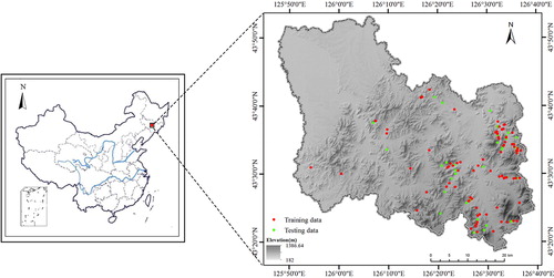
YJC lies in the transition zone between Changbai Mountain and Songnen Plain, and the terrain gradually decreases from south to north. There are seven peaks that are higher than 1000 m above sea level, and most of the peaks from 500 to 1000 m are in the southern and middle areas. There are four landforms in the entire area: the middle mountains, low mountains, platform, and river valley.

According to genetic age, material composition, structure, and physical and mechanical properties, the lithology is divided into the following five categories: relatively hard clastic rock (conglomerate, sandstone, and siltstone), soft clastic rock (shale and tuffaceous shale sandstone), hard bedded rock (limestone), hard massive rock (granite), and soil mass (clay, sub clay, fine sand, coarse sand, and gravel soil). The study area lies in the Tianshan–Xingan geosyncline fold area, Jilin and Heilongjiang fold system. Faults dominantly trending approximately NE–SW and NW–SE are present in this region.

The study area has a continental, dry, and cold monsoon climate in the North Temperate Zone with four distinctive seasons, and the temperature changes significantly. The annual average temperature is 5.3 °C with an annual average precipitation of 722.75 mm. The maximum annual rainfall is 1150 mm (2010), minimum annual rainfall is 457 mm (1982), and rainfall is concentrated between June to August.

2.2. Inventory map

Based on a field survey of the study area, a total of 123 debris flow hazards were identified and are shown in the inventory map (Figure 1). The debris flow disaster that occurred in YJC is mainly distributed across the southeast mountain area, and to a lesser extent in the northwest plain area.

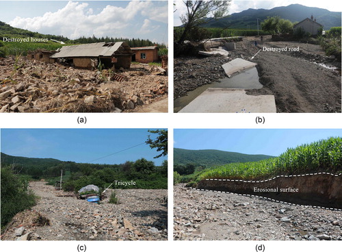
Before July 13, 2017, based on a survey and zoning of 1:50000 geological disasters in the Jilin Province, a total of 91 debris flow disasters were investigated. The debris flow damaged 247 houses and 430 acres of farmland, with a direct loss of 15 million yuan. On July 13 and 19, 2017, two heavy rainstorms occurred in YJC with an average rainfall of 175.4 mm, and the maximum reached 309 mm. The field survey statistics indicated that the rainstorm caused 32 debris flows. The debris flows destroyed roads and houses and caused traffic paralysis and homelessness (Figure 2).

Figure 2. Debris flow disasters identified in the field: (a) destroyed houses; (b) destroyed road; (c) buried vehicle; and (d) destroyed farmland.

In this study, 70% (n = 86) of the debris flows were selected randomly for training data, which were used to create the DFSM models. The remaining 30% (n =37) were used as testing data, which were used to validate the DFSM model (Figure 1).

3. Influencing factors

Occurrence of debris flow is related to a variety of factors. For example, geological, topographical, morphological, and vegetation and human engineering activities can influence debris flows (Chang et al. 2014; Shi et al. 2016; Li et al. 2017). Debris flow factors considered in this study include elevation, slope, precipitation, landforms, lithology, land use, distance to fault, and population density. These factors were used to create the DFSM model, which provided good results (Xu et al. 2013; Elkadiri et al. 2014; Kritikos and Davies 2015; Camilo et al. 2017). The 8 × 8 m digital elevation model (DEM) of study area was collected using the Google Earth. By using this DEM, topographic-related thematic data layers such as elevation and slope were prepared. Precipitation data were collected from weather stations in YJC. The geology parameters were obtained using a geological map of Jilin Province, with a scale of 1:200,000. Other parameters were mainly collected from available resources.

The elevation ranges between 182 and 1386.64 m in the study area (Figure 3a). The elevation reflects the relative height difference, which aids in determining the gravity potential energy of the debris flow. The larger the height difference, the greater the gravitational potential energy. This provides a dynamic condition for the occurrence of a debris flow. For the WU, the difference between the highest and the lowest points in each watershed was calculated and used as influencing factor.

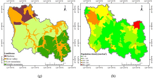
Figure 3. Maps of influencing factors based on GCUs: (a) Elevation; (b) Slope; (c) Precipitation; (d) Distance to fault; (e) Lithology; (f) Land use; (g) Landforms; and (h) Population density.

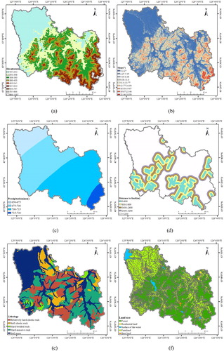
Based on the DEM, the slope was obtained using ArcGIS. Stability of the slope decreases with an increase in slope angle, and a steep slope helps to provide loose materials. The slope also influences the initiation and movement of debris flows (Lin et al. 2002; Chang and Chao 2006) (Figure 3b). For the WU, the average slope in each watershed was calculated.

The precipitation, which is one of the most important factors for triggering the initiation of debris flow, was selected as an influencing factor. Debris flow often occurs during the rainy season (Oh and Pradhan 2011). Clearly, in the study area, heavy rainfall easily induces debris flow. The precipitation in the study area varies between 650 and 730 mm (Figure 3c). For the WU, the rainfall level for each watershed was determined based on the principle of majority, and this principle was also applied to factors of distance to fault, lithology, land use, and landforms.

Earthquakes often occur around the fault, which leads to breakage and weathering of the rocks and formation of a significant weathering zone, thereby providing more materials to the debris flow (Hong et al. 2015). An interval of 800 m is used to generate multiple buffer zones between faults, and these are divided into five classes based on the natural breaks method (Figure 3d).

Strong connection exists between the lithology and formation of debris flows. Lithology controls the stability of slopes and determines the quantity of materials available to a debris flow. The lithology is divided into the following five categories: relatively hard clastic rock, soft clastic rock, hard bedded rock, hard massive rock, and soil mass (Figure 3e).

The type of land use reflects the changes and effects of human activities on nature. In general, agricultural production and residential use destroy the original vegetation, reduce the capacity of soil and water conservation, and provide good conditions for the occurrence of debris flows, and these are integrated into five categories according to the type of land use (Figure 3f).

The debris flow occurs mostly in the mountainous areas, and the conditions of the landform type affect the initiation, movement, and scale of debris flows. There are four major landforms in the study area: platform, river valley, low mountains, and middle mountains (Figure 3g).

The influence of social and economic factors on vulnerability of debris flow should not be ignored. Human activity factors are important triggers for debris flow. In this study, population density was selected as an influencing factor to represent the intensity of human activities (Figure 3h). For the WU, the average population density in each watershed was calculated.

4. Methodology

4.1. Watershed unit extraction based on ArcGIS

The WU division in this study was completed by using Model Builder in ArcGIS. The construction algorithm of the WU is illustrated in Figure 4. The first step involves the depression filling of the original DEM (30 m × 30 m), which is followed by the extraction of the direction of water flow. Further, through the slope runoff simulation method, which is based on the flow direction to calculate the flow accumulation, the threshold is set to connect the cells with a flow accumulation larger than the threshold to form a river grid network, and then, the river network is classified and turned into a vector. Finally, through stream link and watershed range extraction, the WU is divided. In this study, two thresholds, i.e., 10 000 and 5000, were selected. The river nets based on these thresholds are similar to those of the real river. The number of the WUs units is 202 and 394, respectively (Figure 5). The general characteristics of the considered mapping units are listed in Table 1.

Figure 4. Construction process of the WUs: (a) processing flow and (b) interface of WU model builder.

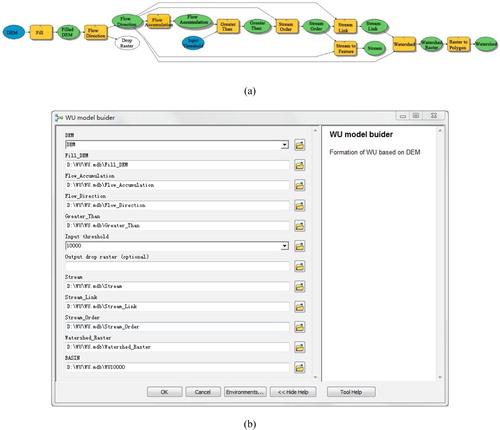
Figure 5. The study area based on GCU (size is 8 m × 8 m) and WUs: (a)–(c) correspond to the GCU flow thresholds of 10 000 and 5000, respectively.

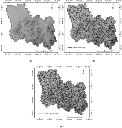
Table 1. General characteristics of considered mapping units.

Mapping units	Number	Average area (m^2)	Minimum area (m^2)	Maximum area (m^2)
GCU	40944392	64	64	64
WU10 000	202	12972480	81000	65372400
WU5000	394	6650865	50400	41517900

4.2. The frequency ratio

The FR method is an accurate and effective method, which is based on the observed relationships between the distribution of debris flows and related factors. In this study, the FR method was used to complete the DFSM (Lee et al. 2007; Park et al. 2013; Rozos et al. 2013). The FR is defined as the ratio of the probability of occurrence of a debris flow to the probability of a nonoccurrence for the given attributes (GF 1994; Regmi et al. 2014). The larger the FR, the stronger the effect of the given factor on the debris flow (Lee and Talib 2005). First, the FR for each factor type or range was calculated, and the corresponding equation is represented as follows: (1) $$\mathit{FR}=\frac{A_1/A_2}{B_1/B_2}$$(1) where $A_1$ is the number of cells with a debris flow disaster for each factor class; $A_2$ denotes the total number of cells with a debris flow disaster occurrence in study area; $B_1$ represents the number of cells for each factor class; and $B_2$ denotes total number of cells in the study area.

Then, the debris flow susceptibility index (DFSI) was calculated by using the following equation: (2) $$\mathit{DFSI}=\sum \mathit{FR}$$(2) where DFSI is debris flow susceptibility index and FR is the frequency ratio of a factor or range. Clearly, the greater the DFSI, the higher the risk of occurrence of debris flow (Lee and Pradhan 2007). Finally, the DFSM is generated based on the DFSI (Jadda et al. 2011). The spatial relationship between debris flow disasters and influencing factors derived from the FR is listed in Tables 2 and 3.

Table 2. Distribution of the training pixels based on GCU.

Factors	Class	No. of Pixels in domain	Percentage of domain	No. of debris flow disasters	Percentage of debris flow disasters	FR
Elevation (m)	181–243	10884765	0.27	1	0.01	0.04
	243–309	8835593	0.22	20	0.23	1.08
	309–380	9211974	0.22	36	0.42	1.86
	380–455	5659620	0.14	22	0.26	1.85
	455–541	3200545	0.08	5	0.06	0.74
	541–644	1778083	0.04	2	0.02	0.54
	644–781	814507	0.02	0	0.00	0.00
	781–966	417544	0.01	0	0.00	0.00
	966–1387	141414	0.00	0	0.00	0.00
Precipitation (mm)	650–675	5418466	0.13	0	0.00	0.00
	675–700	15461202	0.38	8	0.09	0.25
	700–715	17990759	0.44	70	0.81	1.86
	715–730	2153977	0.05	8	0.09	1.77
Slope (°)	0–2.27	14244259	0.35	15	0.17	0.50
	2.27–5.15	7153306	0.17	39	0.45	2.60
	5.15–8.17	5100228	0.12	22	0.26	2.05
	8.17–11.0	4238301	0.10	8	0.09	0.90
	11.0–13.77	3529085	0.09	0	0.00	0.00
	13.77–16.50	2848945	0.07	1	0.01	0.17
	16.50–19.67	2116503	0.05	0	0.00	0.00
	19.67–23.46	1194428	0.03	1	0.01	0.40
	23.46–38.59	518988	0.01	0	0.00	0.00
The distance to Fault (m)	0–800	5970186	0.15	24	0.28	1.92
	800–1600	5491587	0.13	17	0.20	1.48
	1600–2400	4483419	0.11	15	0.17	1.60
	2400–3200	3487681	0.09	9	0.10	1.23
	>3200	21591514	0.53	21	0.24	0.46
Landforms	Platform	3426508	0.08	0	0.00	0.00
	River valley	11189486	0.27	43	0.50	1.83
	Low mountains	16944765	0.41	10	0.12	0.28
	Middle mountains	9383185	0.23	33	0.38	1.67
Lithology	Relatively hard clastic rock	8694653	0.21	6	0.07	0.33
	Soft clastic rock	4537226	0.11	4	0.05	0.42
	Hard bedded rock	826255	0.02	0	0.00	0.00
	Hard massive rock	11691074	0.29	34	0.40	1.38
	Soil mass	15194734	0.37	42	0.49	1.32
Land use	Forest	19307711	0.47	14	0.16	0.35
	Residential land	2100802	0.05	14	0.16	3.17
	Surface of the water	1492035	0.04	0	0.00	0.00
	Farmland	17512158	0.43	57	0.66	1.55
	Bare land	531372	0.01	1	0.01	0.90
Population density (man/km^2)	0–80	19820032	0.48	63	0.73	1.52
	80–140	9846890	0.24	22	0.26	1.07
	140–269	7929089	0.19	1	0.01	0.06
	269–461	2535071	0.06	0	0.00	0.00
	461–2897	895559	0.02	0	0.00	0.00

Table 3. Distribution of the training pixels based on WU 10 000.

Factors	Class	No. of pixels in domain	Percentage of domain	No. of debris flow disasters	Percentage of debris flow disasters	FR
Elevation (m)	0–116	494780	0.17	0	0.00	0.00
	116–223	318359	0.11	2	0.02	0.21
	223–339	463576	0.16	5	0.06	0.37
	339–534	1173216	0.40	34	0.40	0.98
	534–936	461701	0.16	45	0.52	3.30
Slope (°)	0–2.13	483166	0.17	0	0.00	0.00
	2.13–5.20	459622	0.16	3	0.03	0.22
	5.20–8.00	885654	0.30	5	0.06	0.19
	8.00–11.95	896326	0.31	50	0.58	1.89
	11.95–22.30	186864	0.06	28	0.33	5.07
Precipitation (mm)	650–675	388651	0.13	0	0.00	0.00
	675–700	1150591	0.40	8	0.09	0.24
	700–715	1217361	0.42	70	0.81	1.95
	715–730	155034	0.05	8	0.09	1.75
The distance to Fault (m)	0–800	567409	0.19	21	0.24	1.26
	800–1600	231123	0.08	22	0.26	3.23
	1600–2400	169636	0.06	12	0.14	2.40
	2400–3200	110577	0.04	1	0.01	0.31
	>3200	1838527	0.63	30	0.35	0.55
Landforms	Platform	259405	0.09	0	0.00	0.00
	River valley	506673	0.17	3	0.03	0.20
	Low mountains	1374135	0.47	13	0.15	0.32
	Middle mountains	771423	0.26	70	0.81	3.07
Lithology	Relatively hard clastic rock	686647	0.24	20	0.23	0.99
	Soft clastic rock	353252	0.12	8	0.09	0.77
	Hard bedded rock	23795	0.01	0	0.00	0.00
	Hard massive rock	865185	0.30	51	0.59	2.00
	Soil mass	982757	0.34	7	0.08	0.24
Land use	Forest	1642952	0.56	77	0.90	1.59
	Residential land	159	0.00	0	0.00	0.00
	Surface of the water	44787	0.02	0	0.00	0.00
	Farmland	1223734	0.42	9	0.10	0.25
Population density (man/km^2)	0–88	1282857	0.44	62	0.72	1.64
	88–152	930535	0.32	19	0.22	0.69
	152–249	496076	0.17	5	0.06	0.34
	249–439	155783	0.05	0	0.00	0.00
	439–681	52018	0.02	0	0.00	0.00

5. Results

5.1. Evaluation results based on grid cell units

Evaluation results based on GCUs indicate that most debris flow disasters occurred at the elevation of 243–455 m. The FR of elevation classes higher than 644 m is 0. For the slope, debris flow disasters are mainly concentrated at 0°–11°, and a low gradient contributes to the accumulation of a debris flow. In the case of precipitation, the FR values for the classes of 650–675, 675–700, 700–715, and 715–730 are, respectively, 0.00, 0.25, 1.86, and 1.77. Clearly, debris flow mainly occurs in areas where precipitation is more than 700 mm. For the distance to fault criteria, class 0–800 m exhibits the highest FR value of 1. 92, followed by class 1600–2400 m with 1.6, and finally, class 800–1600 m with 1.48. The number of debris flows in the 0–3200 m range accounts for 75.58% of the total flows. In case of landforms, the river valley proved to be the most prone to debris flow disasters with the highest FR value being 1.83, followed by the middle mountains with an FR value of 1.67. Low mountains and platforms exhibited the lowest FR values of 0.28 and 0, respectively. The results of debris flow assessment based on lithology indicated that most debris flows appeared in hard massive rock and soil mass. The FR values of hard massive rock and soil mass are 1.38 and 1.32, respectively. Hard bedded rock is unlikely to form debris flow disasters. Evaluation results of land use based on GCUs reveal that class of residential land has the highest FR value of 3.17, followed by farmland with 1.55. When the vegetation is destroyed in a farmland, a bare surface is created, and soil is scoured by rainwater, which is easily lost; thus resulting in a debris flow. The FR value of forest is 0.35, and forests can reduce soil erosion; thus, the policy of returning farmland to forest should further be improved. For population density, debris flow disasters are mainly concentrated at 0–140 man/km².

According to Formula (2), the DFSM based on GCU is shown in Figure 6a. Based on the natural breaks method (Feizizadeh and Blaschke 2013; Cao et al. 2016), the DFSM was divided into five classes, namely, very low, low, moderate, high, and very high, which is summarized in Table 4.

Figure 6. Debris flow susceptibility mapping based on (a) GCU, (b) WU 10 000, and (c) WU 5000.

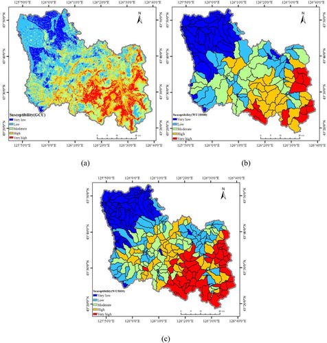
Table 4. The classification of DFSM.

Mapping units	Area (km^2) and ratio (%)	Susceptibility
		Very low	Low	Moderate	High	Very high
GCU	Area	258.40	708.64	767.21	604.42	281.93
	Ratio	9.86	27.04	29.28	23.06	10.76
WU 10 000	Area	689.33	528.31	611.59	543.34	248.02
	Ratio	26.30	20.16	23.34	20.73	9.46
WU 5000	Area	556.08	529.11	469.58	472.47	593.36
	Ratio	21.22	20.19	17.92	18.03	22.64

The above mentioned discussion indicates that the very high and high susceptibility areas for DFSM were found to be located at a high altitude, steep slope, and close to the fault. The lithology in this area was mainly composed of hard massive rock and soil mass. The tectonic movement provided a large amount of loose materials as a source for the debris flows (Wang et al. 2017). The low and very low susceptibility areas accounted for 36.9% of the study area. These regions are lower in altitude and belong to river valley landforms; the terrain is flat, land is mainly farmland, lithology is mainly soil mass, these regions are far from the fault, and there are no debris flows.

5.2. Evaluation results based on the watershed units

In calculating the FR values, two types of WUs present the same trend. There are five classes of elevation, the highest FR value is obtained for the fifth class, and both values are greater than 3.00. With the decrease in the elevation, the FR value is also reduced, and the lowest FR value corresponds to the first class, which is 0.00. The FR results for the slope are similar to those for the elevation, i.e., the higher the slope, the larger the FR value. The two FR values for the fifth class are 5.07 and 3.37 for WU 10 000 and WU 5000, respectively. The FR value for the first class is 0, which is in accordance with the fact that a debris flow does not likely occur on a gentle slope. Regarding the precipitation, the WUs and the GCUs show the same trend, i.e., debris flows occur mainly in class 700–730 mm. Evaluation results for distance to fault reveal that the FR values of the WUs are different from those of GCUs, attributed to larger size of WUs. With respect to land use, the forest has the largest FR value, followed by the farmland. The results of landforms indicate that two types of WUs are consistent and include middle mountains with the highest values of FR. Then, there are low mountains and river valley. The class platform has the lowest FR value of 0. For lithology, two types of WUs are the same, and the highest FR value is for the hard massive rock class with an average value of 2.04. This is followed by relatively hard clastic rock and soft clastic rock. The lowest FR value is obtained for the hard bedded rock class, which is 0. For population density, two types of WUs show the same trend, debris flows are mainly concentrated in sparsely populated areas.

According to Formula (2), the DFSM based on WUs is shown in Figures 7b and 7c. Based on the natural breaks method, the DFSMs based on two types of WUs were divided into five classes: very low, low, moderate, high, and very high. The area of each class is listed in Table 4.

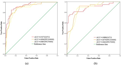
Figure 7. Success and prediction rate curves based on GCUs and WUs for flow thresholds of 10 000 (WU 10 000) and 5000 (WU 5000): (a) success rate curve and (b) prediction rate curve.

For the DFSM, the zone of very high susceptibility has an area of 248.02 and 593.36 km² for WU 10 000 and WU 5000, accounting for 9.46% and 22.64% of the total study area, respectively. Furthermore, the zone of high susceptibility has an area of 543.34 and 472.47 km² for WU 10 000 and WU 5000, accounting for 20.73% and 18.03% of the total study area, respectively. Clearly, the very high and high susceptibility zones are distributed in the southeast part of the study area and the landform in this part is dominated by middle mountains. The elevation, slope, and precipitation values of the very high and high susceptibility zones are large. This region lies close to the faults and it mainly consists of forest and farmland. The lithology of the very high and high susceptibility zones is mainly composed of hard massive rock and relatively hard clastic rock. Moreover, the tectonic movement leads to the weathering of rocks followed by accumulation of as formed loose materials, which turn into debris flow disaster in rainstorm weather. Moderately susceptibility zone is distributed in the middle of the study area and the landform in this part is dominated by low mountains. The area of the moderately susceptibility zone accounts for 23.34% and 17.92% of the research area for the flow thresholds of 10 000 and 5000, respectively. This area mainly consists of forest and the lithology is mostly composed of relatively hard clastic rock. The very low and low susceptibility zones are in the northwest of YJC, and the values of elevation, slope, and precipitation are small. The landforms of this area mainly include river valley and platform. This area is far from the faults and the lithology is mainly composed of soil mass, thus no conditions for forming loose deposits prevail in this region (Guo-liang et al. 2017).

5.3. Validation of the DFSM results

Validation of the DFSM results is one of the most important tasks (Dieu et al. 2011). In this study, the results of DFSMs were validated by the receiver operating characteristic (ROC) technique. In the ROC curve, the vertical axis represents a true positive rate and the horizontal axis represents a false positive rate. The area under the ROC curve (AUC) was used to evaluate the validity of four models. Based on the training and testing data, the success and prediction rates of six models were calculated by using AUC. The value of AUC varied from 0.5 to 1, and the accuracy of the model was high if the value of AUC was close to 1.

Figure 7a displays the accuracy rates for the classification methods of 0.927 for the GCUs and 0.896 and 0.885 for the WU 10 000 and WU 5000, respectively. The associated predicted accuracy rates are 0.888, 0.879, and 0.862, respectively (Figure 7b). This result shows that the three models have high and equal abilities to predict the occurrence of debris flows.

6. Discussion

6.1. Application of frequency ratio

FR is a simple, understandable, and effective probabilistic method, which is widely used in the susceptibility evaluation of geological hazards (Regmi et al. 2014; Cao et al. 2016). In this research, the FR method was adopted to better reflect the characteristics of DFSM based on WUs. By using the ROC curve analysis and AUC, the validation results attested to both the GCU-based susceptibility model and WU-based susceptibility model exhibiting high suitability in the DFSM. The DFSM models used in this research also prove that the FR method has high applicability to evaluating the susceptibility of occurrence of a debris flow. Figures 6a–c indicate that very high and high-risk regions are mainly located in the southeast area of YJC. The disasters caused in the region by debris flows are impossible to estimate, and the local residents should be vigilant during the rainy season.

6.2. Comparative analysis of watershed units and grid cell units

The GCU is the most commonly used disaster susceptibility mapping unit. Compared to the WU, the GCU has larger AUC for both validation procedures (success rate and prediction rate), which shows that the GCU is more accurate and this has been proven in many studies (Wang et al. 2017; Zezere et al. 2017). However, the GCU destroys the integrity of the debris flow; although each GCU has a corresponding geological factor, almost any terrain information space is completely independent (Jia et al. 2012). In contrast, the WU, which is the basic unit of development and activity of a debris flow, can protect the integrity of debris flows and easily reveal the spatial information and geological background of a debris flow. When a single point is used to represent a debris flow, only the geological and geomorphic information at the location of the debris flow disaster is considered based on the GCU. However, the debris flow is composed of a forming area, a circulation area, and an accumulation area, and thus, it is better to consider the effects of geological and geomorphic factors on the formation of debris flows in the entire watershed based on the WU. For example, the weathered granite, which increases the density and destruction force of debris flows, is the main component of debris flows (Figure 2). Debris flows pile up over the soil mass, which results in high value of FR of soil mass based on GCU; however, the FR value of hard massive rock is high based on WUs.

In summary, the rapidity, simplification, and accuracy are the advantages of GCU; however, it is nearly independent of the geologic, geomorphic, or other spatial terrain information. The WU, which is much larger than the GCU, completely considers the geological and geomorphic information of a debris flow and helps to reduce the consequences of existing position errors in a debris flow inventory (Zezere et al. 2017). Furthermore, the watershed is the object of exploration, research, and prevention of debris flows. From the DFSM (Figures 7b and c), it is easy to determine which basin has a relatively large probability to form debris flows and which is relatively safe to put forward targeted defensive measures. However, the WU leads to overestimation of debris flow susceptibility and equilibrium phenomenon exists during the extraction of the influencing factors (Guzzetti et al. 2006).

6.3. Watershed units of different flow threshold

In this study, two types of WUs were selected to map debris flow susceptibility. The extent of very high susceptibility zones derived using WU 10 000 are smaller than that using the WU 5000, while the high, moderate, and very low susceptibility zones determined using WU 10 000 are larger than those by using the WU 5000. The WU 10 000 generates a high AUC for the training group (0.896) in contrast with the equivalent AUC obtained for the WU 5000 (0.885). The AUC decreases when the debris flow test group is considered (Figure 7). However, the WU 10 000 still generates a high AUC for the testing group (0.879) against the WU 5000 (0.862). The model based on WU 10 000 generates higher AUC for the success and prediction rates, but the unit size is very large, and debris flows mostly occur only in very large watersheds (Table 1), which is explained as an overestimation of debris flow susceptibility (Zezere et al. 2017). When the WU is used as the mapping unit of DFSM, a WU that is too large covers most part of an area, which overestimates the debris flow susceptibility and is not significant for the practical prevention and control of debris flows. Thus, a suitable WU should be selected according to the actual situation.

7. Conclusion

DFSM is helpful for disaster management and lays the foundation for the formulation of disaster reduction measures. Based on this idea, in this study we provided the results of DFSM based on three types of mapping units: GCU, and watershed units (WU 10 000 and WU 5000) in YJC, Jilin Province, China. The FR method was used as the statistical method. Elevation, slope, precipitation, landforms, lithology, land use, distance to fault, and population density were selected as the main influencing factors. After many field investigations, a total of 123 debris flow disasters were investigated in the study area, where 70% (86 debris flows) were selected randomly for training and creating the DFSM models. The remaining 30% (37 debris flows) were used for testing and validating the DFSM model. By using the ROC curve and AUC, the effectiveness of the results was verified. In the following study, we will constantly update the debris flow database to increase the data quality.

By using the Model Builder in ArcGIS, a tool for generating WUs was developed, which significantly improves the work efficiency. The WUs of flow thresholds 10 000 and 5000 were selected to map debris flow susceptibility. The results show that the very high and high susceptibility zones are mainly located in the southeast area of YJC.

The model based on GCU, which involves a simple calculation process and shows a stable modelling performance, lacks in physical meaning. In contrast, the WU can reflect the geological and geomorphic environmental conditions of a debris flow accurately and perfectly. From the DFSM of WU, the risk level of each watershed can be determined directly, and targeted measures should be taken to avoid the occurrence of potential debris flow disasters. Based on the actual prevention and control of debris flow disasters, a WU with a suitable size should be selected to complete DFSM.

Acknowledgments

The authors are also thankful to anonymous reviewers for their valuable feedback on the manuscript.

Additional information

Funding

This work was supported by the National Natural Science Foundation of China [grant number 41202197]; Key Projects of the National Natural Science Foundation of China [grant number 41330636]; China Postdoctoral Science Foundation [grant number 20100471265]; National Natural Science Foundation of China [grant number 41807227]; and China Postdoctoral Science Foundation Funded Project [grant number 2017M621212].