Flood map boundary sensitivity due to combined effects of DEM resolution and roughness in relation to model performance

Abstract

In comprehending flood model results, we performed sensitivity analyses and evaluated how different combinations of digital elevation model (DEM) resolution and Manning’s roughness affect flood maps produced from a 2D hydraulic model. Moreover, we analysed how the estimation of accuracy can further be influenced by the performance measure and the area’s topography. Various combinations of DEM and Manning’s $n$ produced different results, in terms of quantified performance in relation to actual flood extent and the generated flood boundaries. High-resolution DEMs performed better with higher Manning’s $n,$ while lower $n$ values were better for lower resolution DEMs. Furthermore, although lower resolution DEMs (25 and 50 m) received higher quantified performances, there are more discrepancies in the flood maps and water surface elevations (WSE) produced by them. The current statistical estimators of model performance do not necessarily provide an accurate estimate of which combination of DEM resolution and roughness are more suitable for application to modelling. Different statistical estimates have different assumptions, which can affect the model selection. Therefore, a more holistic approach towards model selection should be adopted that gives equal importance to statistical estimators, as well as the quality of flood inundation extents.

Keywords:

• DEM
• flood
• GIS
• goodness of fit
• hydraulic modelling
• Manning’s n
• sensitivity analysis

1. Introduction

1.1. Background

In floodplain and flood risk management (FRM), important parameters in assessing risks include the level and extent of the water during the 100-year event. This information serves as input to hazard, vulnerability, and risk maps. Water surface elevations (WSEs) can be derived from gauge measurements along the river during an extreme event. These can be interpolated and the depths can be estimated by subtracting the heights in digital elevation models (DEMs) from the water surface values to acquire both depth and spatial extent of water (Apel et al. 2009). Images from remote sensing can also be used for delineating flooded and dry zones during an inundation event. Satellite images such as the Landsat Thematic Mapper (TM) and Synthetic Aperture Radar (SAR) can be used for distinguishing the reflectance of water from other land features (Wang et al. 2002; Penton and Overton 2007). However, a drawback from these methods is that they do not take into account the flow dynamics in the river and the floodplain. To deal with these, hydraulic modelling has to be performed to simulate flows. The flow simulations performed are dependent on the model used, which has certain assumptions on how the numerical equations are to be applied in routing the water. Simplest in assumptions are one-dimensional (1D) flood models (e.g. HEC-RAS and MIKE-11), which are able to produce good results for well-defined river valleys (Horritt and Bates 2002), and simulate large areas at fine resolution at a faster rate. For more complex rivers and floodplains, two-dimensional (2D) models (e.g. Telemac, LISFLOOD-FP) can be utilised. In these models, topography is represented by contiguous surfaces in the form of mesh or grid.

As flood models have become more widely available (both commercially and for free), and hydrologic data and better resolution DEMs are more accessible, the task of predicting flood events, which is viable for planning, has considerably been eased. Despite this, different studies have also shown how uncertain the results can be due to the effect of the input data, parameters, and boundary conditions used for flow simulations. Two known factors recognized by many to which models exhibit high sensitivity are DEM resolution (Horritt and Bates 2002; Fewtrell et al. 2008; Schumann et al. 2008; Cook and Merwade 2009; Saksena and Merwade 2015), and the roughness coefficient (Horritt and Bates 2002; Mason et al. 2003; Pappenberger et al. 2005; Schumann et al. 2007).

The positive effects of high-resolution data to model outputs have been mentioned, for instance, in Horritt and Bates (2002) and Schumann et al. (2008). Their importance is attributed mainly to producing more detailed topography of the area (Cook and Merwade 2009; Di Baldassarre and Uhlenbrook 2012), which is necessary for representing precise and accurate channel and overland flows in hydraulic analysis (Mason et al. 2003). DEMs produced by LiDAR, in combination with river bathymetry are recognized to provide better model results (Schumann et al. 2008). Nevertheless, high-resolution DEMs are not error-free in producing inundation extents, especially in flatter areas. As shown in Brandt and Lim (2012; 2016) and Brandt (2016), DEMs produce discrepancies in extents when compared to reference data. But unlike coarser resolution DEMs, the uncertainties associated are lower.

For the 1D model the utilisation of fine resolution DEM is easy and fast, whereas for 2D models it is still computationally intensive, especially in big areas to which the modelling is applied. According to Savage et al. (2016), this leads to the limitation of being able to conduct uncertainty analysis, especially Monte Carlo realizations, that will take into account the sensitivity of the model to a wide variety factors, including fine resolution data.

Conversely, the Manning’s $n,$ which represents the surface resistance to the flow, is an important parameter in hydraulic modelling. The n-value used often relies on the characteristics of the test site in terms of the land cover or the type of bed and ground surface material. Different models have shown varying degrees of sensitivity to friction parameters (e.g. Horritt and Bates 2002; Di Baldassarre et al. 2010). One reason is that every model has different assumptions in solving energy losses (Hunter et al. 2007). Another reason is that the sensitivity of the model to the roughness can further be affected by the DEM or mesh resolution (Romanowicz and Beven 2003; Horritt et al. 2006; Yu and Lane 2006; Neal et al. 2009; Savage et al. 2016), boundary conditions (Hall et al. 2005; Pappenberger et al. 2006; Yu and Lane 2006; Savage et al. 2016), and discharge (Aronica et al. 1998; Romanowicz and Beven 2003; Di Baldassarre and Montanari 2009).

To assess model prediction results as outcomes of specific DEM resolution and Manning’s roughness combination usage, performance (goodness-of-fit) measures can be used. They are applied to quantify how well the model predicted the flood at a given event, in comparison to a reference flood boundary. Deterministic flood maps are often derived from the most optimal (i.e. having highest performance) calibration result. Even flood probabilistic (e.g. Aronica et al. 2002; Di Baldassarre et al. 2010) and uncertainty maps (Horritt 2006) are produced on the basis of these performance measures, which are used for deriving the likelihood weights assigned to a given model result from the ensemble modelling, especially in uncertainty assessment following the Generalized Likelihood Uncertainty Estimation (GLUE) (Beven 2009) method. However, there is limited research on how well the performance measures work.

Therefore, the aims of the current study are to evaluate (1) how the predicted extents produced by flood models can be affected by both the DEM resolution and the model parameter (in terms of the Manning’s roughness) used and (2) how the estimation and analysis of model prediction, as well as the choice of optimal maps used for deterministic mapping, can further be influenced by the performance measure used.

1.2. Research issues and contributions

To date, different literature have assessed uncertainties caused by different hydraulic models to either the input data and model parameters/conditions (see e.g. Aronica et al. 2002; Hunter et al. 2005; Pappenberger et al. 2005; Di Baldassarre and Montanari 2009; Mason et al. 2009; Mukolwe et al. 2014). Even so, there remain some issues that are not addressed or not explicitly discussed in the earlier studies, which can be essential, to understand the causes and effects of sensitivity of flood modelling results.

1.2.1. Effects of high and low resolution DEMs in predicted flood model results

When sensitivity analyses of 2D hydraulic models that regards the effects of DEMs in combination with different model parameters/boundary conditions have been made (as in the works of Horritt and Bates 2001; Savage et al. 2016), lower to medium resolution elevation models (i.e. 10 to 50 m) are tested and utilized, whereas DEMs with fine resolution (1–5 m) seldom have been used. This is because it still takes longer time to perform 2D hydraulic model simulations with high-resolution data, especially in larger floodplain and study area. However, as higher resolution data become more available, it is relevant that results based on these models are also analysed, to see how good the predicted flooding is, in terms of performance measure related to the flood extents.

1.2.2. Assessment of results using different performance measures

In assessing model performance and for determining optimal (best) model results that are used in deterministic maps, performance (goodness-of-fit) measures are used to quantify how well a model prediction is in comparison to a reference flood. Each of these goodness-of-fit measures has assumptions on how they quantify model results. In flood extent validation studies, the most common measures are the different forms of feature agreement statistics ($F$), which account for the proportion of flooded and dry areas by either using number of pixels (Aronica et al. 2002; Hunter et al. 2005) or areal size (underestimated, overestimated or overlapping) (Di Baldassarre et al. 2010; Mason et al. 2009; Papaioannou, Loukas, Vasiliades, and Aronica 2016). There are two versions of the $F$-statistics. $F1$ takes into account the overlap size between the modelled and reference flood extents, in relation to the overall predicted and underestimated areal sizes. This was implemented in, e.g. Aronica et al. (2002) and Mason et al. (2009). However, to eliminate the bias in the $F1$ equation, overlap size is penalized by subtracting the size overestimated by the model, leading to the $F2$ equation (Hunter et al. 2005). In Lim et al. (2016), another goodness-of-fit measure was presented that takes into account the error (i.e. disparity) between the model and the reference flood using sampling methods to produce probabilistic and uncertainty flood maps.

Thus, with the different goodness-of-fit methods available, it is therefore vital to evaluate and even compare how the quantified performances will vary among the different measures used as effect of the DEM and Manning’s roughness used. As part of the evaluation, we also propose new methods for quantifying flood extent sensitivity, and compare them with existing methods.

1.2.3. Relating performance measures to flood extents

Although several studies have analysed the combined effect of statistical flood estimators and flood inundation extents in evaluating the performance of hydraulic models, these comparisons are typically done when presenting flood maps from fewer simulation results (e.g. Cook and Merwade 2009; Papaioannou et al. 2016; Yu and Lane 2006). However, in studies implementing Monte Carlo simulations, results are often presented as graphs showing for instance the changes in WSE, discharge, size of flood extent, response to model parameter (Yu and Lane 2006; Neal et al. 2009; Papaioannou, Vasiliades, Loukas, and Aronica 2017) or the performance of the model (e.g. Aronica et al. 2002; Pappenberger et al. 2005). This is because these studies often highlight important trends in the results presented from the ensemble. Graphs and diagrams are therefore practical in presenting numerous amounts of information at the same time and in determining data trends. Additionally, the quantified performance has been an important basis of indicating how good the model produces its results in ensemble modelling. However, these quantities only numerically determine model behaviour, but lack providing spatial overview of the flood extent generated, which can be helpful in understanding where and why variability is lowest or largest at the given geographic location, or the quality of the extents produced. Hence, in the sensitivity analysis results derived in this study, quantified model performance are analysed together with the flood maps.

1.3. Study areas

The two study areas investigated were the Testebo and Voxna rivers in Sweden (Figure 1). The entire Testebo river (Testeboån) is about 85 km long, stretching from Ockelbo municipality to Gävle. The part of the river studied is situated north of Gävle City. The site is about 2.7 km², including the areas of Varva (north and east) and Forsby (west and southwest). The large floodplain in Varva is composed of arable land, while the western portion consists of open areas. Residences, broad-leaf and mixed forests are also visible in some parts of the study site. The river’s mean annual discharge is 12.1 m³/s. Four large spring floods have been recorded for the river in the years 1916, 1937, 1966 and 1977. The most extreme event that took place was in 1966, with a recorded flow of 180 m³/s (Olofsson and Berggren 1966), while the 1977 flood had discharge of 160 m³/s, equivalent to the 100-year flow.

Figure 1. Location of test sites in black: (a) the Voxna river in Edsbyn and (b) the Testebo river north of the city of Gävle. ©Lantmäteriet.

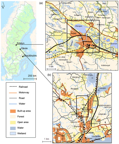
The Voxna river (Voxnan) is 190 km long, flowing through the municipalities of Ljusdal, Ovanåker, and Bollnäs. Its upstream section, which is about 120 km long, is a nature conservation area, making this part of the river to be unregulated. There are several rapids and waterfalls present in this stretch, including the Hylströmmen waterfalls. Surrounding area is dominated by forests and mires. After Hylströmmen, the river meanders. This part is characterized by sand bars. Thereafter, the river continues to flow through the towns of Voxna, Edsbyn, and Alfta, and downstream to its outlet in Lake Varpen, which is part of the Ljusnan river.

The chosen test site is in Edsbyn, measuring about 14.7 km². Edsbyn was identified as one of the most vulnerable areas to flooding in 2011 (Myndigheten för samhällsskydd och beredskap 2011). Two of the biggest floods that happened here were in 1985 and 2000. The former was the worst and caused significant economic losses (Länstyrelsen Gävleborg 2015). The peak flood discharge was 360 m³/s (in Alfta), with almost 3 m raised water level at Ön, which is in the centre of the study area. The Voxna river has a mean annual flow of 39.6 m³/s at the outlet.

2. Methods

2.1. Pre-processing of data

The topographic data used for the Testebo river came from LiDAR and river bathymetric measurements that were available. Both datasets were produced by SWECO (a technical consulting company), where the latter was supplemented by additional interpolated points in areas that were not possible to echo sound (cf. Lim 2009). The original point cloud contained about 4 million ground data points, with an average spacing between 0.20 and 1.8 m, while the channel bathymetry had spacing from 0.5 to 3.6 m. This dataset has horizontal and vertical accuracies of 0.10 m. All bridges were manually removed from the laser scanned data so as not to obstruct the flow of water during the modelling.

The point cloud data used for the Voxna river was produced by Lantmäteriet, the Swedish mapping, cadastral, and land registration authority. Horizontal and vertical accuracies of the laser-scanned data is 0.25 and 0.05 m, respectively. The ground data were extracted from the original point cloud and filtered using FME (https://www.safe.com/). A total of 7 million ground points comprised the final point cloud data used for the test site, making it more manageable to process. The bathymetric data were derived from the Swedish Civil Contingencies Agency (Myndigheten för samhällskydd och beredskap, MSB).

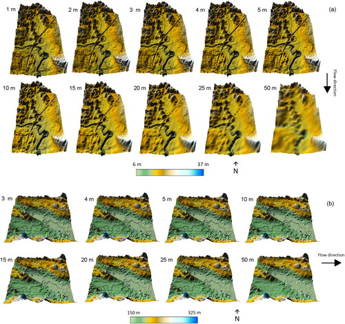
In producing the bare earth DEM that provides the geometry of the study areas, the two point datasets (i.e. point cloud and the river bathymetry) were combined and used to generate a Triangular Irregular Network (TIN) model in GIS. The choice of initially creating a TIN takes advantage of being able to process millions of points at a shorter time, and its capability to provide better river geometry (Vivoni et al. 2005). Because the 2D hydraulic model CAESAR required grid data input for the hydraulic modelling, the TIN results were converted to raster DEMs. In the TIN to raster conversion, elevation values (coming from the TIN) are interpolated using linear interpolation. The interpolation outputs were then assigned the cell sizes of 1, 2, 3, 4, 5, 10, 15, 20, 25, and 50 m (Figure 2a), which were used for the simulations performed for the Testebo river. For the Voxna river, the highest resolution used was 3 m, due to technical limitations of the hydraulic model (Figure 2b).

Figure 2. The different DEMs used for the simulations: (a) the Testebo river and (b) the Voxna river. Direction of flows is shown by the arrows.

The validation data used for Testebo river was provided by the Gävle municipality, showing the extent of the 1977 flood. This was said to be digitised from an aerial photo of the flood with flow equivalent to 160 m³/s. The reference flood extent for the Voxna river, which was also in ESRI shapefile format, was provided by Ovanåker municipality. It covers the extent of the actual flood that took place in September 1985, with a discharge of 360 m³/s.

2.2. Hydraulic simulations and ensemble modelling

CAESAR-LISFLOOD, which is a raster-based model that routes the flow from one cell to another using orthogonal directions (four-direction movement) (Coulthard et al. 2013) to allow faster computation, was used for inundation modelling. Its flow component is based on the modified LISFLOOD-FP model (Bates, Horritt, and Fewtrell 2010). LISFLOOD-FP is characterized as a 1D/2D hydrodynamic model, using full shallow water equations, which is solved for each cell. It integrates inertial effects for faster and more stable flow computations. There are three main equations from the LISFLOOD-FP model implemented in CAESAR for its reach model component. The first equation initially calculates the flow (Q) between cells using flux, acceleration to gravity, Manning's $n,$ depth, elevation, maximum flow depth between cells, and the size of the grid. This discharge is used for computing the second equation, which accounts for the water depth at a given cell location. The last equation adopted is for computing time step, which is also crucial for providing model stability. Here, the grid size, together with the $\mathrm{\alpha }$ coefficient and the celerity value, are used to solve the equation (see Coulthard et al. 2013).

To assess the sensitivity of the model to the effects of the topographic data and roughness parameter, ensemble modelling was performed. In ensemble modelling, multiple simulations are implemented, where conditions vary for each simulation. This leads to producing an ensemble of models, having different results. Each model outcome can then be used for assessing model uncertainty or in determining an optimal model based on the tested conditions (Beven 2009). For this study, 100 and 80 simulations were conducted using different input/parameter combinations of DEMs and roughness coefficient (i.e. 10 DEM resolution $\times$ 10 $n$ = 100 for Testebo river, and 8 DEM resolution $\times$ 10 $n$ = 80 for Voxnan). Motivations for following this design in the ensemble modelling were:

1. the aim of the study is to evaluate model performance as effect of input DEM resolution and the Manning’s roughness parameter used, in terms of their quantified values and the spatial extents of the floods produced. Since the purpose is to conduct a sensitivity analysis that investigates the spatial variabilities of each output map generated, thousands or even hundreds of results may be impractical to use and will only limit the visualisation and comparison of the flood extents.

2. the most common DEM resolutions for flood mapping applications were used. Slight changes in the DEM resolution (i.e. cm changed) may be unrealistic to be utilized. High-resolution DEMs (1$-$5 m for Testebo river, and 3$-$5 m for Voxna), were also included in the test, in addition to commonly tested medium to low resolution DEMs (10, 15, 20, 25 and 50 m); and,

3. a uniform Manning’s roughness applicable for both the channel and the floodplain was used. The range of values tested followed Horritt and Bates (2002), with increments of 0.01.

The reach model of CAESAR-LISFLOOD was implemented in the simulations. The peak flood discharges corresponding to the reference data were used for running steady-state flow simulation (i.e. inflow equals output). The choice of a steady-state simulation was motivated by the length of the reach, and because the maximum flood extent is the main output to be derived (cf. Di Baldassarre et al. 2010). All other parameters were set as constants and determined, respectively, in agreement with CAESAR-LISFLOOD standards (Coulthard et al. 2013).

2.3. Model performance evaluation

In quantifying how well the model performed as result of using different combinations of DEM resolution and $n,$ the flood extents produced from each simulation was compared with the flood extent of the validation data using (1) the two feature agreement statistics (i.e. $F1$ and $F2$) as presented in the studies of Horritt and Bates (2001), Aronica et al. (2002), Hunter et al. (2005), Mason et al. (2009); and (2) central tendency measurements from computed disparities, in terms of the mean (Lim et al. 2016) and median, which is introduced in this paper.

2.3.1. Feature agreement statistics ($F$)

In these goodness-of-fit measures, the modelled flood extent is compared to the observed data (i.e. reference), by utilizing the set theory to denote the number of members in the set that are predicted to be flooded (mod), and observed (obs) flooded (Equation 1(1) $$F=\mathrm{ }\frac{\mathit{Num}(S_{\mathit{mod}}\cap S_{\mathit{obs}})}{\mathit{Num}(S_{\mathit{mod}}\cup S_{\mathit{obs}})}$$(1) ) (Bates and de Roo 2000; Horritt and Bates 2002). Here, the intersection and union between the predicted and observed data are accounted for. (1) $$F=\mathrm{ }\frac{\mathit{Num}(S_{\mathit{mod}}\cap S_{\mathit{obs}})}{\mathit{Num}(S_{\mathit{mod}}\cup S_{\mathit{obs}})}$$(1)

In flood extent validation studies, there are two versions of feature agreement statistics, which were utilized in the study. $\mathrm{F}1$ (Aronica et al. 2002; Mason et al. 2009; Papaioannou et al. 2016) uses Equation 2(2) $$F1= \frac{A_i}{A_i+B_i+C_i}$$(2) to account for model performance. Here, the total size of overlap (${\mathrm{A}}_{\mathrm{i}}$) between the modelled (i.e. the modelled simulation result, i, using a specific combination of DEM resolution and Manning’s roughness) and the reference data is divided by the sum of the overlap (${\mathrm{A}}_{\mathrm{i}}$), and areas over- (${\mathrm{B}}_{\mathrm{i}}$) and underestimated (${\mathrm{C}}_{\mathrm{i}}$). In $\mathrm{F}2$ (Hunter et al. 2005), the size overestimated (${\mathrm{B}}_{\mathrm{i}}$) is subtracted from the overlap, to penalize the overestimation by the model (Equation 3(3) $$F2= \frac{A_i-B_i}{A_i+B_i+C_i}$$(3) ). Both $F$-statistics have values ranging from 0 (no model fit) to 1 (perfect model fit): (2) $$F1= \frac{A_i}{A_i+B_i+C_i}$$(2) (3) $$F2= \frac{A_i-B_i}{A_i+B_i+C_i}$$(3)

2.3.2. Mean ($\overline{D}$) and median ($\stackrel{\sim }{D}$) disparities

With both $F$ statistics, it is difficult to determine how much a simulation result differs from the validation data, as they only give performance based on the total sizes of overlap, and over- and underestimations. Additionally, how large or small the differences are from the reference can also be influenced by local factors or where the surveyed data are measured. Hence, aside from using the feature agreement statistics above, the usage of both mean ($\overline{D}$) and median ($\stackrel{\sim }{D}$) disparities were looked at for quantifying model performance. The possibility of using the latter is also explored in this study as there can be cases, especially with highly skewed data, where the median is more appropriate to be used as measure of central tendency.

In both methods, points ($p$) were sampled from the intersection of the water surface produced in a particular simulation ($i$) result and the cross-section ($m$) (Figure 3, left). The cross-sections were numbered and divided accordingly to left and right parts (looking downstream the channel), using the stream centreline. Each was coded based on its location, which served as its unique identifier when joining the information to the sampled point data. Coordinates ($x$ and $y$) of the samples were then extracted for each point.

Figure 3. Illustration of how the points used for disparity measurements were sampled from one of the simulation results (left) and from the reference data (right) using the cross-sections.

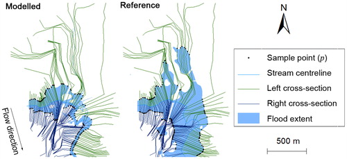
The same procedure was followed when extracting the point samples from the validation data (Figure 3, right). Each point was also identified uniquely according to the cross-section location. It is important that this point location corresponds with that of the simulated flood results in order to perform the computation. The disparity or distance ($D$) (Brandt and Lim 2012) between the sampled points from the modelled result and the reference data (at the same cross-section location $m$) was computed using the $x$ and $y$ coordinates, and by applying Equation 4(4) $$D_{\mathit{pm}}=\mathrm{ }\sqrt{{\Delta x}_{\mathit{pm}}^2+{\Delta y}_{\mathit{pm}}^2}$$(4) : (4) $$D_{\mathit{pm}}=\mathrm{ }\sqrt{{\Delta x}_{\mathit{pm}}^2+{\Delta y}_{\mathit{pm}}^2}$$(4)

To get the model performance of the given simulation, the mean (${\overline{D}}_i$) of the sampled disparities ($D_{\mathit{pm}}$) were derived using Equation 5(5) $${\overline{D}}_i=\frac{\sum D_{\mathit{pm}}}{N}$$(5) . $N$ is the total number of sample points used. For the median (${\stackrel{\sim }{D}}_i$), Equation 6(6) $${\stackrel{\sim }{D}}_i=\frac{1}{2}(D_{\mathit{pm},\frac{n-1}{2}}+D_{\mathit{pm},\frac{n-1}{2}+1})$$(6) was used, as the total N is an even number. If N is an odd number, Equation 7(7) $${\stackrel{\sim }{D}}_i=D_{\mathit{pm},\frac{n-1}{2}}$$(7) should be applied: (5) $${\overline{D}}_i=\frac{\sum D_{\mathit{pm}}}{N}$$(5) (6) $${\stackrel{\sim }{D}}_i=\frac{1}{2}(D_{\mathit{pm},\frac{n-1}{2}}+D_{\mathit{pm},\frac{n-1}{2}+1})$$(6) (7) $${\stackrel{\sim }{D}}_i=D_{\mathit{pm},\frac{n-1}{2}}$$(7)

The point sampling was performed for all the 100 (Testebo) and 80 (Voxna) simulations results to be able to derive their corresponding performances using ${\overline{D}}_i$ and ${\stackrel{\sim }{D}}_i.$ High model performance is estimated to be closer to zero, i.e. lower disparity or difference from the observed flood extent.

3. Results

The combined effects of the input DEM and the roughness parameter on the prediction, as well as the effect of the performance measure in the assessment were analysed through: (1) the spatial variability of the predicted extents from each DEM resolution and Manning’s $n$ combination, in comparison with the reference flood boundaries; (2) the variation in WSE; (3) overall performance of the model using the different goodness-of-fit measures; (4) the highest performing model for each performance measure; and (5) the range of performance for each DEM resolution and roughness coefficient.

3.1. Spatial variability of the extents in comparison with the actual data

Each resulting extent was grouped and mapped according to DEM resolution to find out where the over- and underestimation were highest in each simulation result, and how sensitive the extents were to the given input/parameter used. Based on visual inspection (“eyeball” verification) of Figure 4, it can be seen that regardless of the resolution, all total flooding extents in the Testebo area were underestimated when using Manning’s $n$=0.01 to 0.04, particularly in the northern part (which is characterized by a flatter floodplain), and southern parts of the study area. The variation in extents as effect of the Manning’s $n$ were most evident for the 1 to 5 m resolution DEMs. The difference in extents in these locations were minimized as the resolution became coarser. With $n$=0.01–0.04, the flood in the southern part of the river was also underestimated when using all DEMs. This was with the exception of the 25 m data, which minimally underestimated the southwest portion, and the 50 m data, which gradually produced an overestimation as the $n$ was increased. At $n$=0.05 and 0.06, the northern portion of the area was fully inundated in all resolutions. There were still underestimations in the southern part, but mostly for higher resolution DEMs (1 to 10 m) that were paired with these Manning’s $n.$ With $n$=0.07 to 0.10, the 1977 flood extent was within the predicted extents in all resolution used, though the size of the overestimation in the northern and the entire western parts also became bigger as the roughness values were increased.

Figure 4. Flood extents grouped according to DEM resolution for the Testebo river.

For the Voxna river (Figure 5), it is also noticeable how the total flood extents were underestimated, particularly in the southeastern part of the study area, when high-resolution DEMs (from 3 to 5 m) were paired with lower Manning’s $n.$ The fit between the model and the reference became better with higher friction coefficient, especially between $n$=0.07 and 0.08. From 10 m resolution and worse, it can be visually seen that the southeastern portion was already inundated, even with the lowest roughness values. The model also produced an overestimation of the flood in this location, as compared with the reference data.

Figure 5. Flood extents grouped according to DEM resolution for the Voxna river.

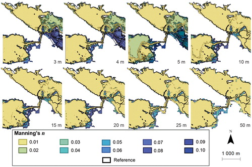
The different flood maps also show how the details in topography are represented in the extents when data changed from higher to lower resolution. For the 1 to 5 m data, the ditch feature at the north of the Testebo river was shown to be flooded when using lower Manning’s values (0.1 to 0.05). However, these details were lost in the lower resolution data. Also, the appearance at the borders of the flooding becomes blockier starting from the 10 m DEM. With the 50 m, much of the details at the edges were already lost. There were also bigger extents of the flooding produced with this resolution regardless of the $n$ that was used.

3.2. Effects of DEM resolution and manning’s n on the water surface elevation

In Figures 6 and 7, WSEs for both study areas are plotted for different cross-sections characterized by steep side slope (CS #10 and #32) and flat topography (CS #42 and #14), respectively. The reason is to be able to see if there will be changes in the WSE, which could have also affected the lateral expanse of the water at these two sites. It can generally be seen that water levels increased with increased Manning’s $n,$ regardless of the test site. Different resolution also caused differentiation in the water level. However, how big the difference was depended on the cross-section location. For Testebo river’s CS #42 (Figure 6), WSE became more varied as a result of different resolution data, but was highest for the coarsest DEMs (25 and 50 m). This was brought by the increase in bed elevation, particularly in the floodplain. Although the terrain became more irregular with the 5 and 10 m data, the bed elevation was still at the same level as the 1 m DEM. In CS #10 (which is characterized by narrower channel bounded by steep side slopes), despite the increase in bed elevation for the 25 and 50 m DEMs, the width of the channel also increased, making the cross-sectional area where the water flows almost similar to the higher resolution DEMs.

Figure 6. The water levels produced from using different resolution DEMs and Manning’s $n$ for two coss-sections characterized by steep (CS #10) and flat (CS #42) side slopes in the Testebo river.

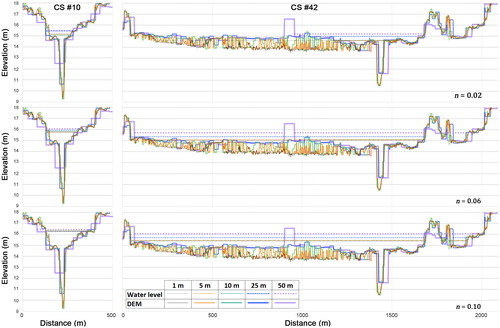
Figure 7. Cross-sectional profiles of the Voxna river. CS #32 is from a location bounded by steep-side slope, while CS#14 was from a flatter part of the river.

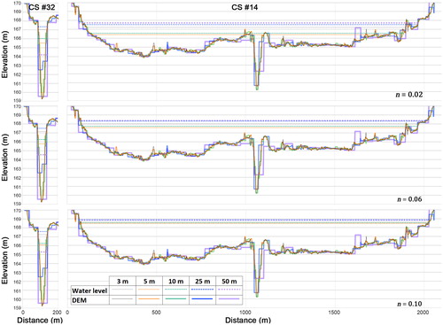
The cross-sectional pattern for Voxna river is similar to Testebo in terms of the changes in the topography and channel widths as effect of the DEM, and how the sizes of cross-sectional areas were compensated by these two factors (Figure 7). Unlike the Testebo river, the channel part of Voxna is deeper. In its narrower part (CS #32), the water remains confined in the channel even when the highest Manning’s $n$ was used. With the 50 m DEM, the thalweg did not differ much from the higher resolution DEMs, but it made the channel broader in this location as effect of the grid size. Hence, this produced a lower WSE, although the cross-sectional areas (in all Manning’s $n$) produced by this DEM are larger than the rest of the results. The effect of increased bed elevation to the water level has been more evident for the 25 m data in this location. For the flatter part of the channel (CS #14), the peak discharge of 360 m³/s has already brought about much water in this area in all Manning’s n conditions. It can also be seen that with the different DEMs, the water is bounded by steeper side slopes, causing it to increase more vertically than laterally, compared with a cross-section with gentler side slopes. Moreover, in this part of the river, there were lesser alterations in the topography as effect of the DEM, particularly for higher resolution DEMs. Nevertheless, the 25 and 50 m data have produced more modifications in the elevation, by raising the channel bed, and smoothening the floodplain topography.

3.3. Overall model performance

The overall performances of the models using all the DEM and Manning’s $n$ combinations for the different goodness-of-fit measures are shown in Figure 8. The maximum possible performance using $F1$ and $F2$ is 1, while for the disparities, a lower mean or median indicates better model performance.

Figure 8. Performance contours for the feature agreement statistics ($F1$ and $F2$) and the two disparity measures (mean disparity, $\overline{D};$ and median disparity, $\stackrel{\sim }{D}$) for simulation results from (a) Testebo and (b) Voxna rivers. High model performances are represented by lighter brown colour, while low performances are darker.

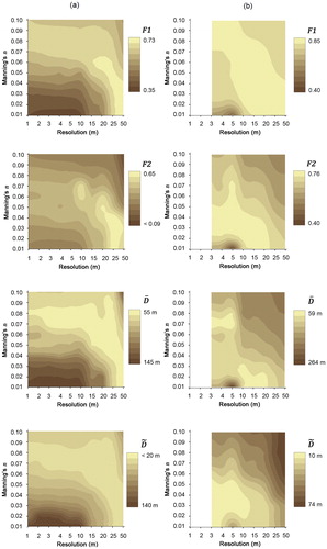
Almost the same pattern can be seen in all four performance measures for the Testebo river (Figure 8a). High to medium resolution DEMs (1–10 m) that were paired with lower Manning’s $n$ produced the weakest performances (dark brown colours). Nonetheless, these resolutions worked well with Manning’s $n\mathrm{ }$between 0.06 and 0.09. The 25 m data showed minimal change in performance in all Manning’s roughness paired with it, although, this decreased gradually as the Manning’s $n\mathrm{ }$was increased. As with the 50 m data, good performance was manifested with the low Manning’s $n$ (0.01 to 0.05), whereas the performance significantly decreased with roughness values from 0.06. The pattern also reveals that the concentration of highest performance (lightest colour) was most evident for the 25 and 50 m resolution, when paired with the different Manning’s $n.$

For the Voxna river (Figure 8b), higher and medium resolution DEMs performed better in general, considering the four performance measures (light yellow, Figure 8b). This was the case for 10 to 20 m data, mainly when paired with lower roughness values. With 25 and 50 m, the performance became lower (with the exception of $F1$) especially as the roughness coefficient was increased. Unlike the Testebo river, the higher resolution DEMs (3 to 5 m) performed better when paired with a wider range of Manning’s values.

3.4. Size variation in modelled flood

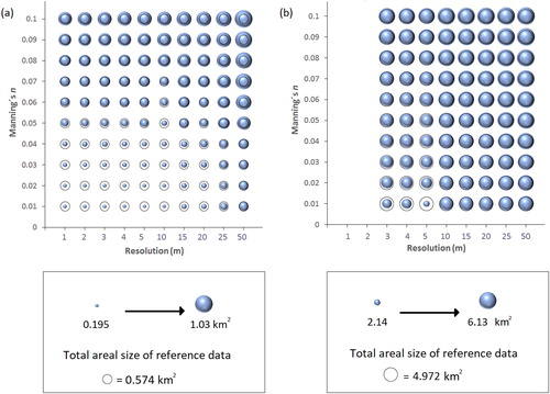
The areal size generated from the simulation result (blue) using each parameter combination is compared with the size of the actual flood extent (the black circles, about 0.574 km² for the Testebo river, and 4.972 km² for the Voxna river,) in Figure 9. Generally, it can be seen from the diagram that the simulation results’ sizes increased with increasing Manning’s $n$ and coarser DEM resolution. Underestimation of the flood extent was common for Testebo river’s results when using lower friction coefficient (0.01–0.5) paired with DEM resolutions from 1 to 20 m. Overestimation of the extent occurred with all DEM resolutions that were paired with roughness values larger than 0.8, in addition to size increase from higher to lower resolution. Best fit models in terms of the size were attained for higher resolution DEMs (from 1 to 5 m) that were paired with $n$=0.07. For the 50 m data, the overall size of the actual and the modelled extents was almost the same when using lower $n$ values (0.01–0.04), but from 0.05, the size of the flooded area increased with the friction coefficient used. For the Voxna river, although higher resolution DEMs produced underestimation of total flood extents when using lower Manning’s values (0.01–0.05), the total sizes did not differ much from the reference data. At $n$=0.06, there is a better match in size, but after this value, the extents became larger. Resolutions from 10 to 50 m had flood size results comparable to the reference when using lower Manning’s coefficient. For the 10 to 20 m, this size was attained when paired with $n$=0.01 and 0.02, but afterwards, the size became bigger than the reference. For the 25 and 50 m, the lowest roughness value already produced a bigger flood extent than the reference data.

Figure 9. Size differences between the simulated (blue) and the actual (black outline) floods for (a) the Testebo river and (b) the Voxna river. Underestimation of the actual flooding is occurring when the black circle is larger than the blue one, while overestimation is occurring when the blue is larger than the black outline.

3.5. Optimal model results from the different performance measures

A comparison of flood extents quantified by the least and highest goodness-of-fit-measures are shown in Figure 10. Least performing simulations from all three measures showed big underestimations of areas to be flooded when compared with the actual flood event, while one result was based on overestimation. All simulations that received the minimum performance for the Testebo river had Manning’s $n$ of 0.01 and 0.1, but the resolution that was paired with the former varied to the different measures used ($F{1}_{5\mathrm{m}}$=0.331; ${\overline{D}}_{10\mathrm{m}}$=144.22 m; and, ${\stackrel{\sim }{D}}_{3\mathrm{m}}$=139.42 m). For the Voxna river, the 5 m and $n$=0.01 received the least performance in three measures while the 50 m paired with the highest Manning’s $n$ was the least when using $\stackrel{\sim }{D}.$

Figure 10. Variations in extents produced for the least (top) and most (bottom) optimal performances for Testebo river (a) and Voxna river (b).

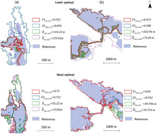
The highest performing models also differed for the performance measure utilized. For the Testebo river, the 5 m and lower resolution DEMs (25 and 50 m) received the most optimal performances, while for the Voxna river, the 5 and 10 m performed the best. However, even with the best performing models for both study areas, it can be observed that no exact match of extents was attained with the reference data. The most optimal model for the Testebo river using $F1$ yielded performance of 0.73 for 50 m, $n$=0.03 (outlined as red in Figure 10a, right). It shows an underestimation of the inundated zone in the north and an overestimation in the southwest. When using $F2,$ the best model was quantified to have performance of 0.651 for the 25 m DEM and $n$=0.04. The model with the highest performance using $\stackrel{\sim }{D}$ generated a larger flooded area (0.79 km²) than $\overline{D}$ (0.64 km²), particularly in the northern and southern portions of river. This was brought by the resolution of the input DEM (${\stackrel{\sim }{D}}_{25\mathrm{m}}$=19.82 m;$\mathrm{ }{\overline{D}}_{5\mathrm{m}}$=55.22 m), as $n$ was 0.07 for both. For the Voxna river, the most optimal performances with the 5 m data (regardless of the Manning’s $n\mathrm{ }$used), showed an underestimation, particularly in the southeastern part of the reach. The best performing result according to$\mathrm{ }F1\mathrm{ }{(F1}_{10\mathrm{m},\mathrm{ }0.04}$=0.85), although inundating the southeastern part, produced an overestimation.

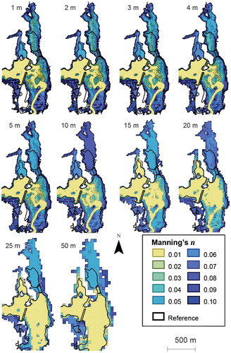
3.6. Highest performance per resolution

The flood extents of highest performing models for respective resolutions are presented in Figures 11 and 12. Most optimal models when using $F1,$ $\overline{D}$ and $\stackrel{\sim }{D}$ for the Testebo river were derived similarly for DEM resolutions of 1–5 m, paired with Manning’s roughness of 0.07 and 0.08 (Figure 11). In these combinations, the overestimation in the north was prominent. There were also underestimations in the flooded areas in the southwest, which also increased with the 3–5 m data. For the lower resolution DEMs, the extents varied more according to both the Manning’s $n$ and the goodness-of-fit measure used for quantifying the performance. The 50 m data in particular performed best with the lowest Manning’s $n.$ It was also shown that when using lower resolution DEMs, extents produced were underestimated in the north.

Figure 11. Flood extents for the highest performing DEM resolution and Manning’s $n$ combinations for the Testebo river.

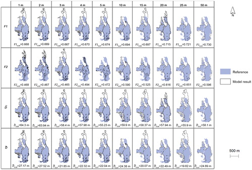
Figure 12. Flood extents for the highest performing DEM resolution and Manning’s $n$ combinations for the Voxna river.

The most optimal result combination produced from $F2$ differs from the other performance measures, especially for higher resolution DEMs (1, 2, 4 and 5 m). With this performance measure, there were more underestimations particularly in the southern portion of the study area for these resolutions. This underestimation in the south became minimal as the resolution became lower (10, 20, 25 and 50 m). Nevertheless, this was compensated by the northern portion being underestimated in the 10–50 m resolution. Also, when using F2, the roughness values paired with the different DEMs were mostly $\le$0.050 (except for the 3 and 10 m DEMs which performed best with $n$=0.07).

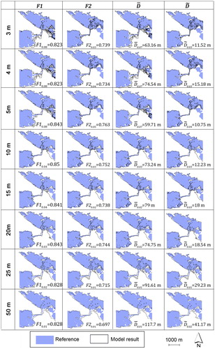
For the Voxna river (Figure 12), the pattern for best performing models for high-resolution DEMs (3 $-$ 5 m) were similar for $F1$ and $\overline{D},$ and $F2$ and $\stackrel{\sim }{D}.$ With $F1$ and $\overline{D},$ these DEMs performed higher with $n$=0.07 and 0.08, while when using the latter measures, quantified performances were higher when they were paired with Manning’s $n$=0.03$-$0.05. Nonetheless, with DEMs 10–$5$0$$ m, all performance measures performed well with lower Manning’s values. For the 10 and 15 m data, Manning’s $n$=0.03 and 0.04 provided the best results, while for 20, 25 and 50 m, roughness values from 0.01 to 0.03 were better.

3.7. Performance ranges per DEM and manning’s n

The minimum, maximum, and the range of performance values were derived for each result using the various goodness-of-fit methods (Figure 13). For the DEMs used in the Testebo river, the differences between the minimum and maximum performances were largest for 1 to 10 m resolutions, whereas they were smaller for the intermediate to lower resolution when using the $F1,$ $\overline{D},$ and $\stackrel{\sim }{D}$ measures-of-fit. Also remarkable to note is that the 25 m DEM was least varied in the performance in these three measures, and also received the highest mean among the different resolution data. On the other hand, when using $F2,$ the pattern was inverted, whereby higher resolution DEMs became the least varied in quantified performance. However, the 25 m DEM again got the highest mean performance, while the 50 m had the least.

Figure 13. Interval plots for the DEM and Manning’s $n$ for the Testebo (a) and Voxna (b) rivers. The mean performance for each resolution/Manning’s $n$ is marked as blue square.

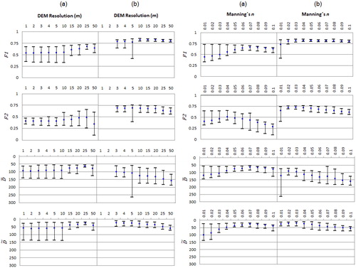
In the Voxna river, there was lesser variability in minimum and maximum performances for all resolutions, with the exception of the 5 m DEM. Although the 5 m data received high maximum performances for the three goodness-of fit-measures ($F2,$ $\overline{D}$ and $\stackrel{\sim }{D}$), this also resulted to the highest performance range due to its results when paired with the lowest Manning’s value. The highest resolution DEMs (3 and 4 m) also received better mean performance ($F2,$ $\overline{D}$ and $\stackrel{\sim }{D})$ than the lower resolution DEMs.

For the Manning’s $n$ used in the Testebo river, the differences in performances for $F1$ were most evident for roughness values between 0.01 and 0.05, whereas higher $n$ values produced significantly lower differences (Figure 13). Similar results were found for both $\overline{D}$ and$\mathrm{ }\stackrel{\sim }{D}$ for the lowest $n$ (0.01 to 04), although the highest roughness value (0.10) also produced a varied performance. Hence, from $n$=0.04 or 0.05 to 0.09, the differences were smaller, especially when 0.07 (for $F1$ and $\overline{D}$) and 0.06 ($\stackrel{\sim }{D})$ were used. With $F2,$ lower mean performances were derived from $n$=0.01 to 0.03, while the highest were from $n$=0.04 to 0.05. When Manning’s $n$ became bigger, the performance decreased.

With Voxna river, it can be noticed that $F1$ and $\stackrel{\sim }{D}$ produced higher and less variable performances for the different roughness values. With $F1$ (except for n = 0.01) all performances were greater than 0.73. The concentration of optimal mean performance was with the Manning’s coefficient 0.02 and 0.03 when using $F2,$ $\overline{D}$ and $\stackrel{\sim }{D},$ while for $F1$ it ranges from 0.02 to 0.07. After these values, the performance decreased, but how big depended on the quantification method used. In F1, this is smaller compared with $F2,$ $\overline{D}$ and $\stackrel{\sim }{D}.$

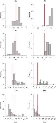
Assuming that a threshold performance is assigned to model results that are to be considered acceptable, the number of simulations that will fall within the threshold values can also depend on the goodness-of-fit measure used. To show how this can be affected by the performance measure, histograms were derived for the different measures (Figure 14) using a threshold of $F\ge$0.50 for both feature statistics and $D\le$50 m for both disparity measures. With $F1,$ the majority of the simulations for the Testebo river (i.e. 74 out of 100) will be acceptable, while for $F2,$ only 18% will be accepted. With the mean disparity, all simulations will not be accepted as the maximum performance was 55.2 m, while 67% will be accepted using the median disparity. For the Voxna river’s results, both F-statistics will only reject one simulation (out of 80) that is below the threshold. Similar to Testebo river, the mean disparity measure will reject all simulations (because of low maximum performance, i.e. 59.7 m), while with median disparity, 77.5% will be accepted.

Figure 14. Histogram of performance measures for the 100 simulation results of the Testebo river (a), and the 80 simulation results of the Voxna river (b). The dashed line represents using the threshold of $F\ge$0.50 and $D\le$50 m.

4. Discussion

In this paper, we investigated the sensitivity of flood extents produced by 2D hydraulic models to the DEM and Manning’s roughness values used. Although the topographic data has significant influence on hydraulic modelling’s results (Saksena and Merwade 2015), the Manning’s roughness remains an important model variable that determines flow resistance. When creating an inundation flood model, the roughness is used to calibrate and fine tune the model to attain high feature agreement statistics. This study, therefore, looks deeper into the dependency between the roughness and resolution of the DEM.

In the hydraulic modelling conducted, steady-state simulations were implemented as this study compares the maximum flood extent with the observed flood boundary. This is similar to the assumption presented in Di Baldassarre et al. (2010) when they used steady-state simulation with 2D modelling for the same purpose. Thus, a similar study using unsteady flow hydrograph as flow input may produce different results from what were derived (also cf. Savage et al. 2016). However, even when an unsteady flow hydrograph is used as upstream boundary condition, it seems that channel friction is the most influential factor on the general flood extent during the time of peak flow (Savage et al. 2016). Although Savage et al.’s (2016) study did not see DEM resolution as particularly important when assessing the global sensitivity of their models (they used 10–50 m resolution), they did stress that “a finer model resolution may be necessary if a decision-maker is interested in local‐scale inundation predictions” (p. 9159).

4.1. Assessment of model performance and extent analysis

The sensitivity of the models to both DEM and roughness parameters were analysed through the different performance measures used. Each of these methods indicate varying best (overall) performing results from the entire ensemble of models produced (Figure 9), and for each resolution and Manning’s $n$ combination (Figures 11 and 12), and study area. If the general trend shown by the different performance values in the diagrams for each parameter pair and for each DEM (Figure 8) will be looked at, they seemed to agree with each other in indicating the concentration of high or low performances for each test site.

The performance measures used and evaluated in this study consider the totality of the flooding generated by the model in comparison to the reference data. They only take into account the lateral expansion of water. Performance based on feature agreement statistics is determined by accounting for the overall changes in the total sizes of areas underestimated, overestimated, and overlapping between the model and the reference data. In $F1$ (Equation 1(1) $$F=\mathrm{ }\frac{\mathit{Num}(S_{\mathit{mod}}\cap S_{\mathit{obs}})}{\mathit{Num}(S_{\mathit{mod}}\cup S_{\mathit{obs}})}$$(1) ), if the size of overlap (A) is equal to the combined sizes of overestimated (B) and underestimated (C) areas by the model, this will lead to $F1=$0.5. If the combined sizes of overestimation and underestimation is smaller than the overlap size, then the performance will be greater than 0.5, while larger combined size will lead to performance lesser than 0.5. Thus, as long as the overlap is larger than the combined areal sizes of the under- and overestimation, a high $F1$ value can be derived. This is the reason why $F1$ performed well for the Voxna river (with almost all simulations producing $F1>$0.64) compared with the Testebo river. For the Testebo river, an exact overlap match between the reference and the modelled results was more difficult to attain, particularly at the northern part of the study area (Figure 9). On the other hand, the results from $F2$ (Equation 3(3) $$F2= \frac{A_i-B_i}{A_i+B_i+C_i}$$(3) ) are affected by the size of overestimation. Negative performance is derived if it is higher than the overlap between the model and the reference, while it will be 0 if they are equal. High performance can be derived if the size of overlap is large and the over-estimation is small, as in the case of the Voxna river. While if overestimation is large relative to the size of overlap, then the quantified performance will become low, which is similar to the results of the Testebo river. This can be a problem in flat areas, which can produce higher model uncertainties, resulting to lower computed performance values. Furthermore, since $F2$ imposes the penalty caused by overestimation that is often produced by using higher Manning’s $n,$ better performance will be assigned to lower roughness values. Both $F$ measures also focus on sizes, and do not account for positional accuracies of the overlaps.

Other variations of feature statistics can also be looked at to be able to see how the performances and the choice of combinations of DEM and Manning’s $n$ used can be affected by these estimators. Table 1 shows a comparison of results if two variants of feature agreement statistics are used. In ${F2}_U,$ instead of penalising the overlap produced by the model by the size of over-estimation (Equation 3(3) $$F2= \frac{A_i-B_i}{A_i+B_i+C_i}$$(3) ), the size of underestimation is used. This equation also results to negative performance if the underestimation is greater than the size of overlap, while 0 is attained if underestimation equals the overlap size. It can be seen that in both study areas, higher Manning’s roughness (particularly for higher resolution DEMs in Testebo river) produced better performances because underestimation is minimized and the overlap is increased. This produces an opposite result to $F2,$ wherein a much lower Manning’s $n$ becomes better because the equation tries to suppress the overprediction by the model. With another feature agreement statistics ($F3$), $\frac{A_i-B_i-C_i}{A_i+B_i+C_i},$ overlap size is penalized by both over-and underestimation. This produces similar optimal combinations of DEM and Manning’s roughness as $F1$ for both the Testebo and Voxna rivers. However, the performance values were different because of the penalty imposed in the numerator. To get performance greater than 0.5, the numerator should be more than half the size of the denominator. Thus, even if the size of the overlap between the model and the reference is large, the performance values will be affected if it has been reduced to less than half the combined sizes of overlap, and over- and underestimation (i.e. denominator), after subtracting the sizes of over- and underestimation. This is the case why the values for the Testebo river were all below 0.50 using this measure. Hence, an$\mathrm{ }F3$-value close to 1 indicates a very strong agreement between modelled and true flood boundary.

Table 1. Comparison of best performance results among different variants of feature agreement statistics, for the Testebo and Voxna rivers.

	Testebo				Voxna
Res. (m)	$F1$	$F2$	${F2}_U$	$F3$	$F1$	$F2$	${F2}_U$	$F3$
1	0.668[n=0.08]	0.468[n=0.05]	0.607[n=0.10]	0.337[n=0.08]	–	–	–	–
2	0.669[n=0.08]	0.467[n=0.05]	0.601[n=0.09]	0.339[n=0.08]	–	–	–	–
3	0.667[n=0.08]	0.465[n=0.07]	0.604[n=0.09]	0.333[n=0.08]	0.823[n=0.08]	0.739[n=0.03]	0.787[n=0.09]	0.646[n=0.08]
4	0.670[n=0.07]	0.494[n=0.04]	0.608[n=0.09]	0.340[n=0.07]	0.823[n=0.08]	0.734[n=0.04]	0.787[n=0.09]	0.647[n=0.08]
5	0.674[n=0.07]	0.472[n=0.04]	0.605[n=0.09]	0.348[n=0.07]	0.843[n=0.08]	0.763[n=0.05]	0.802[n=0.08]	0.687[n=0.08]
10	0.694[n=0.07]	0.590[n=0.07]	0.622[n=0.08]	0.388[n=0.07]	0.85[n=0.04]	0.752[n=0.03]	0.807[n=0.04]	0.700[n=0.04]
15	0.697[n=0.06]	0.525[n=0.04]	0.638[n=0.08]	0.395[n=0.06]	0.841[n=0.04]	0.738[n=0.02]	0.805[n=0.06]	0.682[n=0.04]
20	0.715[n=0.06]	0.616[n=0.05]	0.630[n=0.08]	0.430[n=0.06]	0.843[n=0.03]	0.744[n=0.02]	0.803[n=0.04]	0.686[n=0.03]
25	0.721[n=0.04]	0.651[n=0.04]	0.645[n=0.07]	0.446[n=0.04]	0.828[n=0.02]	0.715[n=0.01]	0.790[n=0.03]	0.655[n=0.02]
50	0.730[n=0.03]	0.596[n=0.03]	0.646[n=0.01]	0.460[n=0.03]	0.828[n=0.01]	0.697[n=0.01]	0.793[n=0.03]	0.657[n=0.01]

For disparities ($\overline{D}$ and $\stackrel{\sim }{D}$), they will depend on the sampling employed, which is performed at each cross-section location. The mean disparity is mainly affected by the maximum disparities measured from the entire sample of a given simulation, and the number of samples having these maximum values. If there are multiple samples having large differences, a higher mean is expected to be derived. Also, as the sampling is based on the cross-sections, the values are sensitive to the positioning of cross-section. If none of the cross-sections are placed in an area where big discrepancies between the modelled and the observation data are found, then a lower overall mean disparity is expected. Moreover, as the sampling results in all simulations having highly skewed disparities to the right because of fewer locations having extremely large disparities, $\stackrel{\sim }{D}$ was a more appropriate measure than the $\overline{D}.$ The median produced lower values in this case, but the overall pattern on how sensitive the results were similar to the mean.

The sampling performed using the cross-section locations in the two disparity measures also assumed a non-2D flow between the two points where the disparities were measured, since they were originally used for assessing 1D model results. Thus, the flow pattern between the actual and modelled extent in the current study (which utilized a 2D model) may not be best represented by the sampling performed at each cross-section. A 2D-based sampling method that traces the path of water over the continuous surface between the two points for measuring disparity, can be an alternative approach.

In the quantification of model performance, the validation data played significant roles when accounting for sizes ($F1$ and $F2$) and disparities ($D_{\mathit{pm}},$$\mathrm{ }\overline{D},\mathrm{ }\stackrel{\sim }{D}$) as these were what the models were compared to. But any reference data can also have further accuracy issues associated with them, which may impact the results of the performance analysis, particularly when using flood extents. For example, when computing disparity (Equation 4(4) $$D_{\mathit{pm}}=\mathrm{ }\sqrt{{\Delta x}_{\mathit{pm}}^2+{\Delta y}_{\mathit{pm}}^2}$$(4) ), distance was measured between the simulated and the reference data using the extracted $x$ and $y$ coordinates of the points at their positions. In the production of the reference data (i.e. its conversion to digital GIS data) positional inaccuracies (Goodchild 1993) can arise. Digitising a real flood event from an aerial photo can cause generalisation problems with respect to how the lines were drawn or how precise they match the edge of the actual flood lines. This is regardless of how the digitisation is performed (manually by hand or extracted/classified by software from an image). Since the measurement relies on the position of the flood boundary, the computation can be affected. How big or small the impact to the performance measure is, depends on the quality of the reference data. Evaluating the accuracy or quality of reference data is beyond the scope of the current study, but one must be aware of how this can impact the computations.

4.2. Optimal roughness values

Despite the two study areas having predominantly similar land covers in the floodplain (i.e. mostly short grasses and cultivated soil in arable lands, and trees), the best roughness values varied with the DEM resolution, the study site and the performance measure used (cf. 4.1 for discussion). Nevertheless, the general trend manifested by both rivers is that higher roughness values between 0.07 and 0.08 performed well with higher resolution DEMs (1 to 10 m for Testebo river, and 3 to 5 m for the Voxna river), while coarser resolution DEMs performed better using lower friction coefficient. The optimal $n$ value derived for higher resolution DEMs is at least twice as big compared with normal $n$-values for natural rivers, given in reference text books and recommended for natural channels in Sweden (i.e. 0.033). As the case also deals with the 100-year flood, big areas surrounding the river will be inundated, which in general, have higher roughness than the actual river beds, due to for example presence of bushes, trees and other objects. These particular areas, which consist of big slack water, may become difficult to model, leading to greater variations in which $n$ is the optimal to correctly represent the real roughness. The effect of roughness can also depend on the model used. Models can show varying degrees of sensitivities to the Manning’s values (cf. Bates and de Roo 2000), because of the different assumptions they have in solving the energy loss equation using the friction coefficient (Hunter et al. 2007). This can result to finding different optimal roughness, as what is exemplified in Horritt and Bates (2002) when they tested HEC-RAS, Telemac and LISFLOOD. Hence, these $n$-values should not be taken as something generally applicable to all rivers. Every model needs to be calibrated and evaluated with the actual river at hand.

Also in the current study conducted, there was only one friction value that was used, representing both the channel and the floodplain, since the flow is considered mainly to be overland at the given discharge. It is possible that the results will vary if a separate channel $n$ is used, as in Hall et al. (2005), where they state that a model is more sensitive to channel than floodplain friction.

4.3. Flood extent and water surface elevation variations

The performance analysis also benefitted from being able to compare the results with the different WSEs produced. An analysis of WSE can help account for the vertical inaccuracies in the results, which will be difficult to determine with the extents. Since the inaccuracies in the DEMs elevations affect the water level, changes in water depths may influence the expansion of the water and the inundation pattern (Saksena and Merwade 2015). It will also be advantageous to perform depth validation with actual data aside from the extent analyses (Pappenberger et al. 2005). However, this is not available for our study sites. The WSE analysis became helpful in our case, in addition to the extent analysis. Relying only on the performance measure to determine optimal model results can lead to the conclusion that lower resolution DEMs can produce better results, and even high performances comparable to high-resolution DEMs, as what was shown in Figures 9–12. However, looking at the corresponding output maps from the optimal models using low resolution DEMs showed loss in details and more mismatches with the borders of the reference data. The most optimal results using higher resolution DEM provided better representation of the flooding and were more accurate at the boundaries in relation to the contours of the terrain. This was also manifested in the results presented in Saksena and Merwade (2015) where higher resolution DEMs produced better quality flood maps than lower resolution DEMs. Furthermore, the WSE outputs for these DEMs using coarser grids may not be reliable as can be seen in the results in Figures 6 and 7, due to the errors in the topography (cf. Section 4.4) produced during the processing of the DEM. For this reason, it can be misleading to only rely on the quantified performance of the model, without visually inspecting the output maps, as well as the water elevations generated by them. As there seems to be a general trend that low resolution DEMs produce higher elevation and water surfaces, it is therefore logical that lower friction values are needed to get higher performance.

4.4. Topographic data processing effect in the flood prediction results

The DEMs that were used in this study and how they were produced, are of importance for the representation of the topography, as they can be derived in different ways, from the initial LiDAR preparation (e.g. reduction of point cloud, removal or addition of feature, interpolation, choice of feature resolution) up to its final conversion to the format required by the model. The topographic data is also prepared separately from the hydraulic model, mainly through GIS techniques. Yet this is also important to be understood from the hydraulic modelling point of view, because the topography is an important simulation input, which interacts with the hydraulic model parameters (i.e. roughness).

As stated earlier, after the TIN was produced, this had to be converted to a raster (through linear interpolation), since the hydraulic model used for this study required gridded topography inputs. This process can lead to some information loss during the conversion. During the interpolation process, the elevation values from the triangular surface facets of the TIN are approximated to the raster cells, and since the two have different data structures, this will affect the accuracy of the values of the elevation, and in turn the water levels and expanse of flooding. This can be compensated by using a high-resolution raster in the conversion to be able to represent the topography similarly to the TIN. For our study, this TIN-to-raster conversion produced smoother and higher bed elevation as the resolution became coarser, which was most obvious for the 25 and 50 m DEMs. This is the same to the effect of DEM resampling to the bed elevation and water depth described and shown in Saksena and Merwade (2015). How significant the effect was, depended on the local terrain, i.e. whether the cross-section analysed is characterized by steep-sided valleys with narrower channel, or by flat areas. In the former, there can be smaller variations in the WSE, like in the Testebo river. Although the bed elevation became higher with coarser resolution, the width of the channel also increased as effect of the grid size. The original width of the channel in this case was almost half the width of the 50 m cell. So this increase in width compensated the rise in the river bed. As mentioned by Cook and Merwade (2009), the effect of coarser grid size can be big for narrower channels, but the effect of elevation inaccuracies (i.e. the increase in bed elevation) in the inundation extent may be insignificant due to being bounded by steeper side slopes preventing the water to laterally expand. In flatter areas, the increase in WSEs became apparent with both increase in Manning’s $n$ and resolution. In Figures 6b and 7b, it can be seen that the terrain became varied (with peaks) as the resolution became lower. In the 5 and 10 m data for the Testebo river, the irregularities in the terrain, particularly the dips, acted as storage for the water. But when it comes to the 25 and 50 m data (in both study areas), the river beds and some parts of the floodplain were raised, and the terrain became smoother. They caused the WSE to become significantly higher than those produced with higher resolutions DEMs. This result again confirms the findings of Cook and Merwade (2009), and Saksena and Merwade (2015) about coarser DEMs generating higher WSE and increasing the inundation width. The influence of coarsening the DEM to the bottom elevation was also shown in the examples provided in Peña and Nardi (2018). However, in their study, they used low resolution DEMs (from 150 to 700 m) because they have larger study areas compared with the investigated sites, which are more local. In the cross-section profiles of the 150 m and 400 m DEMs they used, the increase in bed elevation can be seen. At 400 m, all the details in the terrain were already removed, including the channel. However, all performances that they derived (using $F1$) were all high despite the irregularities in the DEMs (i.e. $F{1}_{150\mathrm{m}}$=0.917; $F{1}_{400\mathrm{m}}$=0.744). This can be explained by the reference data that they used for validation, which was based on a 150 m resolution inundation model.

It is also important to mention that there is a big time difference between the historic flood events (1977 and 1985), from which the reference extents were derived and the surveying conducted to produce the point cloud and bathymetric data. The geographical characteristics of the area when the historic flooding occurred can be different from the current topographic data. In a span of 20+ years there can be changes in the topography. Thus, the modelling extent results, which are based on a different topographic characteristic (i.e. from more recent LiDAR and bathymetric data) can be different from the observed historical flood boundaries. This can contribute to a reason why it is difficult to attain exact inundation match with the reference data.

5. Conclusion

In this study, we quantified and analysed 2D hydraulic model performance of simulated flood extents using different combinations of DEM and roughness coefficient for two study areas (the Testebo and Voxna rivers). Despite that the rivers are unique and the analysis results differ between them, the general sensitivity patterns for the two study areas are similar. Various combinations showed different best model results, which became dependent on the goodness-of-fit measure used. Overall, lower resolution DEMs received high mean quantified performances, while the higher resolution DEMs received more varied results depending on the Manning’s roughness paired with them. Nevertheless, even if intermediate and lower resolution DEMs received higher performance in the extent analysis, these performance measures may not be good determinants of how well the model behaves. As shown in the results, horizontal, as well as vertical inaccuracies in the flooding can further be affected by coarsening the resolution. In this case, coarser resolution DEMs (particularly 25 and 50 m), produced higher bed elevation, which led to an increase in the WSE, and the extent, particularly in flatter areas. Therefore, prediction results need to be investigated spatially to see how the actual map result looks like. Basing model results on goodness-of-fit methods alone may not be sufficient, since they have their assumptions in the equations they apply for calculating performance. However, with the use of a feature agreement statistics, which considers both under- and overestimated flooded areas, better estimates of uncertainties can be derived compared with using only the traditional feature agreement statistics $F1$ and $F2.$ Moreover, by adding the analysis with disparity measures, the uncertainty estimates can get even more precise. Looking at the vertical pattern of the flooding in relation to the topography is also necessary to further understand if there are changes, particularly in the water surface, as effect of both the DEM and model parameter.

Finally, the results derived for this study were based on different assumptions implemented, particularly in the GIS processing method for the derivation of the DEM, hydraulic modelling performed and the performance evaluation methods used. There are also certain limitations, for example in the validation data, in terms of their accuracies and timeliness, which were discussed in the paper. Hence, the results’ analyses and conclusions can be limited by these factors.

Acknowledgement

We would like to thank the reviewers for their suggestions and comments that helped us improve our paper.

Disclosure statement

No potential conflict of interest was reported by the authors.

References

- Apel H, Aronica GT, Kreibich H, Thieken AH. 2009. Flood risk analyses—how detailed do we need to be?. Nat Hazards. 49(1):79–98. doi:10.1007/s11069-008-9277-8
- Aronica G, Bates PD, Horritt MS. 2002. Assessing the uncertainty in distributed model predictions using observed binary pattern information within GLUE. Hydrol Process. 16(10):2001–2016. doi:10.1002/hyp.398
- Aronica G, Hankin B, Beven K. 1998. Uncertainty and equifinality in calibrating distributed roughness coefficients in a flood propagation model with limited data. Adv Water Resour. 22(4):349–365.
- Bates PD, de Roo APJ. 2000. A simple raster-based model for flood inundation simulation. J Hydrol. 236(1–2):54–77.
- Bates PD, Horritt MS, Fewtrell TJ. 2010. A simple inertial formulation of the shallow water equations for efficient two-dimensional flood inundation modelling. J Hydrol. 387(1–2):33–45. doi:10.1016/j.jhydrol.2010.03.027
- Beven KJ. 2009. Environmental modelling: an uncertain future. Boca Raton, FL: CRC Press.
- Brandt SA. 2016. Modeling and visualizing uncertainties of flood boundary delineation: algorithm for slope and DEM resolution dependencies of 1D hydraulic models. Stoch Environ Res Risk Assess. 30(6):1677–1690. doi:10.1007/s00477-016-1212-z
- Brandt SA, Lim NJ. 2012. Importance of river bank and floodplain slopes on the accuracy of flood inundation mapping. In: Murillo Muñoz R., editor. River flow 2012. San José, Costa Rica: CRC Press/Balkema (Taylor & Francis); p. 1015–1020.
- Brandt SA, Lim NJ. 2016. Visualising DEM-related flood-map uncertainties using a disparity-distance equation algorithm. In: Schumann AH, editor. Proceedings of the International Association of Hydrological Sciences (IAHS): The spatial dimensions of water management - Redistribution of benefits and risks. Bochum, Germany: Copernicus; p. 153–159. doi:10.5194/piahs-373-153-2016
- Cook A, Merwade V. 2009. Effect of topographic data, geometric configuration and modeling approach on flood inundation mapping. J Hydrol. 377(1–2):131–142. doi:10.1016/j.jhydrol.2009.08.015
- Coulthard TJ, Neal JC, Bates PD, Ramirez J, de Almeida GAM, Hancock GR. 2013. Integrating the LISFLOOD-FP 2D hydrodynamic model with the CAESAR model: implications for modelling landscape evolution. Earth Surf Process Landforms. 38(15):1897–1906. doi:10.1002/esp.3478
- Di Baldassarre G, Montanari A. 2009. Uncertainty in river discharge observations: a quantitative analysis. Hydrol Earth Syst Sci. 13(6):913–921.
- Di Baldassarre G, Schumann G, Bates PD, Freer J, Beven K. 2010. Flood-plain mapping: a critical discussion of deterministic and probabilistic approaches. Hydrol Sci J. 55(3):364–376. doi:10.1080/02626661003683389
- Di Baldassarre G, Uhlenbrook S. 2012. Is the current flood of data enough? A treatise on research needs for the improvement of flood modelling. Hydrol Process. 6:153–158. doi:10.1002/hyp.8226
- Fewtrell TJ, Bates PD, Horritt MS, Hunter N. 2008. Evaluating the effect of scale in flood inundation modelling in urban environments. Hydrol Process. 22(26):5107–5118. doi:10.1002/hyp.7148
- Goodchild MF. 1993. Data models and data quality: problems and prospects. In: Goodchild MF, Parks BO, Steyaert LT, editors. Environmental modeling with GIS. New York, NY: Oxford University Press; p. 94–103.
- Hall JW, Tarantola S, Bates PD, Horritt MS. 2005. Distributed sensitivity analysis of flood inundation model calibration. J Hydraul Eng. 131(2):117–126.
- Horritt MS. 2006. A methodology for the validation of uncertain flood inundation models. J Hydrol. 326(1–4):153–165. doi:10.1016/j.jhydrol.2005.10.027
- Horritt MS, Bates PD. 2001. Effects of spatial resolution on a raster based model of flood flow. J Hydrol. 253(1–4):239–249.
- Horritt MS, Bates PD. 2002. Evaluation of 1D and 2D numerical models for predicting river flood inundation. J Hydrol. 268(1–4):87–99.
- Horritt MS, Bates PD, Mattinson MJ. 2006. Effects of mesh resolution and topographic representation in 2D finite volume models of shallow water fluvial flow. J Hydrol. 329(1–2):306–314.
- Hunter N, Bates PD, Horritt MS, De Roo APJ, Werner M. 2005. Utility of different data types for calibrating flood inundation models within a GLUE framework. Hydrol Earth Syst Sci. 9(4):412–430. doi:10.5194/hess-9-412-2005
- Hunter N, Bates PD, Horritt MS, Wilson MD. 2007. Simple spatially-distributed models for predicting flood inundation: a review. Geomorphology. 90(3–4):208–225.
- Hunter N, Horritt MS, Bates PD, Wilson M, Werner M. 2005. An adaptive time step solution for raster-based storage cell modelling of floodplain inundation. Adv Water Resour. 28(9):975–991. doi:10.1016/j.advwatres.2005.03.007
- Gävleborg L. 2015. Riskhanteringsplan för översvämning av Voxnan/Edsbyn.
- Lim NJ. 2009. Topographic data and roughness parameterisation effects on 1D flood inundation models. Sweden: University of Gävle.
- Lim NJ, Brandt SA, Seipel S. 2016. Visualisation and evaluation of flood uncertainties based on ensemble modelling. Int J Geogr Inf Sci. 30(2):240–262. doi:10.1080/13658816.2015.1085539
- Mason DC, Bates PD, Dall’ Amico JT. 2009. Calibration of uncertain flood inundation models using remotely sensed water levels. J Hydrol. 368(1–4):224–236. doi:10.1016/j.jhydrol.2009.02.034
- Mason DC, Cobby DM, Horritt MS, Bates PD. 2003. Floodplain friction parameterization in two-dimensional river flood-models using vegetation heights derived from airborne scanning laser altimetry. Hydrol Process. 17(9):1711–1732. doi:10.1002/hyp.1270
- Mukolwe MM, Di Baldassarre G, Werner M, Solomatine DP. 2014. Flood modelling: parameterisation and inflow uncertainty. Water Management. 167(WM1):51-60. doi:10.1680/wama.12.00087
- Myndigheten för samhällsskydd och beredskap (MSB) 2011. Identifiering av områden med betydande över svämningsrisk.
- Neal JC, Bates PD, Fewtrell TJ, Hunter N, Wilson MD, Horritt MS. 2009. Distributed whole city water level measurements from Carlisle 2005 flood event and comparison with hydraulic model simulations. J Hydrol. 368(1–4):42–55.
- Olofsson S, Berggren O. 1966. Redogörelse För Utförda Observationer av Vattenstånd i Testeboån på Sträckan Strömsbro––Åbyggeby under Våren. 1966
- Papaioannou G, Loukas A, Vasiliades L, Aronica GT. 2016. Flood inundation mapping sensitivity to riverine spatial resolution and modelling approach. Nat Hazards. 83(S1):117–132.
- Papaioannou G, Vasiliades L, Loukas A, Aronica GT. 2017. Probabilistic flood inundation mapping at ungauged streams due to roughness coefficient uncertainty in hydraulic modelling. Adv Geosci. 44:23–34. doi:10.5194/adgeo-44-23-2017
- Pappenberger F, Beven KJ, Horritt MS, Blazkova S. 2005. Uncertainty in the calibration of effective roughness parameters in HEC-RAS using inundation and downstream level observations. J Hydrol. 302(1–4):46–49.
- Pappenberger F, Matgen P, Beven KJ, Henry J-B, Pfister L, Fraipont P. 2006. Influence of uncertainty boundary conditions and model structure on flood inundation predictions. Adv Water Resour. 29(10):1430–1449.
- Peña F, Nardi F. 2018. Floodplain terrain analysis for coarse resolution 2D flood modelling. Hydrology. 5(4):52. doi:10.3390/hydrology5040052
- Penton DJ, Overton IC. 2007. Spatial modelling of floodplain inundation combining satellite imagery and elevation models. In MODSIM 2007 International Congress on Modelling and Simulation. Modelling and Simulation Society of Australia and New Zealand (pp. 74–80).
- Romanowicz R, Beven K. 2003. Estimation of flood inundation probabilities as conditioned on event inundation maps. Water Resour Res. 39(3):1061-1073. doi:10.1029/2001WR001056
- Saksena S, Merwade V. 2015. Incorporating the effect of DEM resolution and accuracy for improved flood inundation mapping. J Hydrol. 530:180–194. doi:10.1016/j.jhydrol.2015.09.069
- Savage JTS, Pianosi F, Bates PD, Freer J, Wagener T. 2016. Quantifying the importance of spatial resolution and other factors through global sensitivity analysis of a flood inundation model. Water Resour Res. 52(11):9146–9163. doi:10.1002/2015WR018198
- Schumann G, Matgen P, Cutler MEJ, Black A, Hoffmann L, Pfister L. 2008. Comparison of remotely sensed water stages from LiDAR, topographic contours and SRTM. ISPRS J Photogram Remote Sensing. 63(3):283–296.
- Schumann G, Matgen P, Hoffmann L, Hostache R, Pappenberger F, Pfister L. 2007. Deriving distributed roughness values from satellite radar data for flood inundation modelling. J Hydrol. 344(1–2):96–111.
- Vivoni ER, Ivanov V, Bras Rafael L, Entekhabi D. 2005. On the effects of triangulated terrain resolution on distributed hydrologic model response. Hydrol Process. 19(11):2101–2122. doi:10.1002/hyp.5671
- Wang YJ, Colby D, Mulcahy KA. 2002. An efficient method for mapping flood extent in a coastal floodplain using Landsat TM and DEM data. Int J Remote Sens. 23(18):3681–3696.
- Yu D, Lane SN. 2006. Urban fluvial flood modelling using a two-dimensional-wave treatment, part 1: mesh resolution effects. Hydrol Process. 20(7):1541–1565.