Potential of hybrid evolutionary approaches for assessment of geo-hazard landslide susceptibility mapping

Abstract

As a prevalent disaster, landslides cause severe loss of property and human life worldwide. The specific objective of this study is to evaluate the capability of artificial neural network (ANN) synthesized with artificial bee colony (ABC) and particle swarm optimization (PSO) evolutionary algorithms, in order to draw the landslide susceptibility map (LSM) at Golestan province, Iran. The required spatial database was created from 12 landslide conditioning factors. The area under curve (AUC) criterion was used to assess the integrity of employed predictive approaches. In this regard, the calculated AUCs of 90.10%, 85.70%, 80.30% and 76.60%, respectively, for SI, PSO-ANN, ABC-ANN and ANN showed that all models have enough accuracy for simulating the LSM, although SI presents the best performance. The landslide vulnerability map obtained by PSO-ANN model is more accurate than other intelligent techniques. In addition, training the ANN with ABC and PSO optimization algorithms conduced to enhancing the reliability of this model. Note that, a total of 76.72%, 23.96%, 30.55% and 5.37% of the study area were labeled as perilous (High and Very high susceptibility classes), respectively by SI, PSO-ANN, ABC-ANN and ANN results.

Keywords:

• Geo-hazard zonation
• landslide susceptibility mapping
• geographic information system
• artificial neural network
• hybrid evolutionary algorithms

1. Introduction

Landslide is one of the disasters that have a very complex natural phenomenon. Landslide susceptibility map (LSM) is the first step that needs to be taken for risk assessment and landslide hazard mitigation. During the last three decades, landslide gained a lot of attention, due to the damages caused by this catastrophe worldwide. In a rough estimation performed Iranian Landslide Working Party (2007), about 187 people have been killed every year by landslides (Pourghasemi et al. 2012b). Different landslide assessment techniques have been implemented to compute the landslide susceptibility values (LSVs) (e.g. in a particular study area) (Youssef et al. 2015; Balamurugan et al. 2016; Vakhshoori and Zare 2016). The most influential factors in calculating LSV are elevation, aspect, slope, curvature, soil type, lithology, distances of predefined cells to faults, rivers and roads, land use, stream power index (SPI), topographic wetness index (TWI). Numerous researchers such as Pradhan (2010) and Hong et al. (2016) have argued, and introduced formulas or LSM to provide a reliable approximation with the likelihood of landslide occurrence in the future. Many attempts and cases studies (Parsons et al. 2014; Chaytor et al. 2016; Meng et al. 2016; Yavari-Ramshe and Ataie-Ashtiani 2016) has been applied in the focal point of estimating landslide hazard zonation maps or deformation of large scale structures (Zou et al., 2018). LSM can be a reliable way to have an estimation of a special place, if only this work implement by proper procedure and real dataset, and also in an appropriate working scale (Dong et al. 2017). One of the most efficient usages of LSMs can be their influences on expanding land use planning and residential areas in the future to evade exposing psychological and financial consequences and damages (Pourghasemi et al. 2012a). Because of the huge troubling of relocating people from their own home (Mokoena and Musakwa, 2018; Hoque Mozumder et al., 2018), up to now various tools and methods are used to estimating landslide susceptibility for different study areas. Among these researches, such as Baeza and Corominas (2001) and Moayedi et al. (2011), were based on simple methods like statistical index (SI), frequency ratio (FR) or regression methods. Wang et al. (2015) developed the LSM of Qianyang County of China using the index of entropy (IOE) and certainty factor (CF) models. In this work, they considered fifteen landslide triggering factors, namely slope angle, slope aspect, general curvature, plan curvature, profile curvature, altitude, distance to faults, distance to rivers, distance to roads, the sediment transport index, the SPI, the TWI, geomorphology, lithology, and rainfall. Based on their findings, CF outperformed IOE with a respective prediction accuracy of 82.32% and 80.88%. Chen et al. (2015) compared the applicability of SI, FR and IOE models for landslide hazard analysis in Baozhong Region of China. In this study, 70% of the marked landslides were selected for training the methods, and the remaining 30% landslides were used to calculate the areas under the curve (AUC) index to evaluate the accuracy of each model. Accordingly, the highest prediction accuracy obtained for FR map with 84.95% accuracy, followed by the SI map with 82.37% and IOE map with 82.05% accuracy.

Also, to achieve more accurate results, application of soft computing techniques is reported in many studies (Lee et al. 2004; Lian et al. 2013; Shahri 2016; Gao et al. 2018c, 2018d). Pradhan and Lee (2010) applied a back-propagation (BP) neural network on the measured data points of landslides in Cameron Highland, Malaysia. They estimated the possibility of landslides with an accuracy rate of 83%. They have used other soft computing techniques as a capable tool for landslide hazard zonation (Arora et al. 2004; Farrokhzad et al. 2011). In another case, Oh and Pradhan (2011) used ANFIS tool with four membership functions, including triangular, trapezoidal, generalized bell and polynomial; and introduced ANFIS as a very useful tool in regional landslide susceptibility assessment. Recently, many studies have been done to represent a comparison of different developed models. For example, Pourghasemi et al. (2016) analytical hierarchy process (AHP) and fuzzy logic (FL) methods were compared, and finally, FL was known as a more successful method by 89.7% accuracy. In other similar cases, the AHP model was used for landslide hazard mapping (Pourghasemi et al. 2012b; Althuwaynee et al. 2014; Chen et al. 2016). Also, in recent years, new techniques and optimizing algorithms are used to model an LSM (Chen et al. 2017a; Hong et al. 2017). Chen et al. (2017b) examined the capability of genetic algorithm (GA), differential evolution (DE) and particle swarm optimization (PSO) synthesized with the adaptive neuro-fuzzy inference system (ANFIS) for landslide spatial modelling in Hanyuan County of China. Referring to the acquired AUC values, they introduced the ANFIS-DE (AUC = 0.844) as the most accurate ensemble data mining technique, compared to ANFIS-GA (AUC = 0.821), and ANFIS-PSO (AUC = 0.780).

As explained supra, evolutionary algorithms have been extensively used to enhance the performance of various predictive models. According to the best knowledge of authors, however, ABC and PSO algorithms have been designed in many studies to remedy the shortcomings of intelligent models (e.g. SVM and ANFIS) (Cheng and Hoang 2015; Bui et al. 2017; Chen et al. 2019), no prior attempt has focused on comparing the capability of this technique in performance improvement of ANNs for landslide hazard assessment. Therefore, in this research, we applied ABC and PSO algorithms to a typical artificial neural network (ANN) to improve its applicability for landslide hazard mapping at the northern district of Golestan province, Iran. The capability of the mentioned models (ANN, ABC-ANN, PSO-ANN) was evaluated by comparing the obtained results with actual landslide locations. In this regard, 20% of total landslide cases were used to calculate the AUC index. Remarkably, the input dataset contains elevation, slope degree, lithology, rainfall, SPI, TWI, distance to road, distance to the river, land use, slope aspect, soil type, and plan curvature; where the output was taken LSV. In what follows, section 2 describes the study area, data preparation and statistical analysis of them is presented in section 3, the detailed description of the used models is given in section 4, and the outcomes are presented and discussed in section 5, and eventually, the conclusion is expressed in section 6.

2. Study area

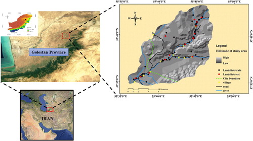
The study area is located in Kalaleh County, Golestan province, Iran (Figure 1). Golestan is one of the northernmost provinces in Iran and is in the neighborhood of the Caspian Sea. The area of the selected region is roughly 163 km² and lies between 37°34′ to 37°44′ N and 55°35′ to 55°47′ E, longitude and latitude, respectively. The district is under the Mediterranean climate chiefly, and the difference between the highest and lowest reported annual rainfall reaches 59 mm per year. Most of the area contains law slope values so that slopes more than 40° are rarely observed. Topographically, the altitudes (i.e. elevation) varies in the range of 200–890 m, and the majority of the area is covered by Calciustepts and Xerorthents soil units. This is noteworthy that the majority of the observed slope failures cover an area <100 m² (10 × 10 m²) and are categorized as ‘rotational’ and ‘translational’ slides. As is clearly shown in Figure 1, most of the landslides have occurred along the territorial roads and rivers, as well as the location of the villages. Note that, no significant fault has been recognized in the purposed study area.

Figure 1. Location of the study area and spatial distribution of landslide inventories.

3. Data preparation and landslide conditioning factors

Landslide is a prevalent disaster in Iran, especially in northern parts of the country, due to the dominant climate condition. In any kind of landslide phenomena modelling, providing the landslide inventory map is the most substantial step (Ercanoglu and Gokceoglu 2004). In this work, this map was acquired through the aerial photos interpretation and extensive field survey using GPS in 1:25,000 scale (see Figure 1). Considering the region climatology, 12 of geological and hydrological factors (e.g. landslide-triggering factors) have been listed as independent parameters in ArcGIS, which were: elevation, slope degree, lithology, rainfall, SPI, TWI, distance to road, distance to river, land use, slope aspect, soil type and plan curvature (see Figure 2). All of the mentioned GIS layers were converted to raster format by 10 × 10 m² cell size to achieve appropriate formats. The elevation map of the area was derived from the digital elevation model (DEM) of Golestan. Minimum altitude value is 200 m and altitudes more than 750 m are rarely observed (see Figure 2(a)). Terrain slope map was subsequently produced from DEM in the range of 0°–43° (see Figure 2(b)). According to lithology distribution map, this region is constructed from five types of rocks. As it is illustrated in Figures 2(c) and 3(a), more than 93% of this region is based on the Swamp sedimentary rocks. Other parts are represented by different rock categories like shale and sandstone, bedded limestone and dolomite and Ammonite bearing shale with the interaction of orbitolina limestone. In the field of land utilization, as is depicted in Figures 2(i) and 3(b), 13 cases of utilization have been reported. However, 82.37% of the area is stratified as mixing of agriculture, forest, rangeland, etc. Furthermore, to investigate the effects of geo-morphometric conditions, two of widely used secondary factors, namely the TWI and SPI were also calculated. TWI measures the amount of water that accumulates in a place, and it is defined by Equation (1)(1) $$\mathit{TWI}=\mathit{ln}\hspace{0.17em}\left(\alpha /\text{tan}\hspace{0.17em}\beta \right)$$(1) (Moore et al. 1991): (1) $$\mathit{TWI}=\mathit{ln}\hspace{0.17em}\left(\alpha /\text{tan}\hspace{0.17em}\beta \right)$$(1)

Figure 2. input data layer maps: (a) elevation, (b) slope degree, (c) lithology, (d) rainfall, (e) SPI, (f) TWI, (g) distance from road, (h) distance from river, (i) land use, (j) slope aspect, (k) soil type and (l) plan curvature.

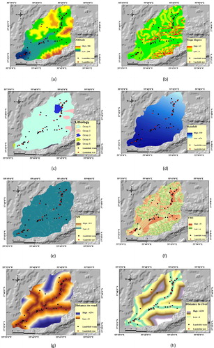
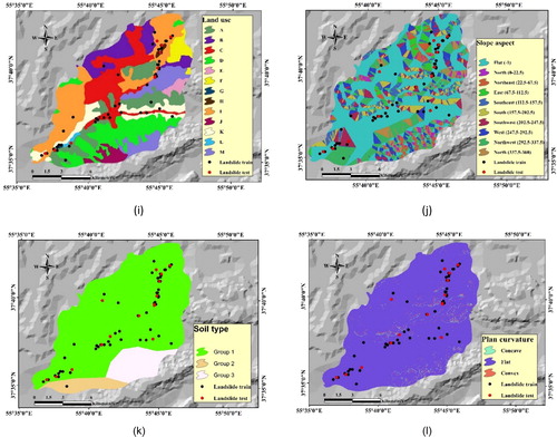
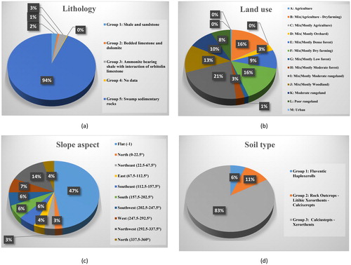
Figure 3. Description and distribution of the nominal parameters: (a) lithology, (b) land use, (c) slope aspect and (d) soil type.

In the above formula, α is the cumulative catchment area, and β defines the slope (see Figure 2(f)). Also, SPI as a topographic attribute indicates the erosion power of a stream is defined in Equation (2) (2) $$\mathit{SPI}=\alpha \times \hspace{0.17em}\text{tan}\hspace{0.17em}\beta$$(2) based on the equation presented by Moore et al. (1991); (2) $$\mathit{SPI}=\alpha \times \hspace{0.17em}\text{tan}\hspace{0.17em}\beta$$(2) where, similarly, α stands for specific catchment and β defines as the gradient (see Figure 2(e)).

Two parameters which relate to the effect of proximity to linear phenomena including roads and rivers (i.e. distance to road and distance to the river) are acquired through applying ‘Euclidean distance’ tool on vector lines in ArcMap (Pradhan and Lee 2010). For these factors, distance varies from 0 to 4234 m and 0 to 4230 m, for roads and rivers, respectively (see Figure 2(g,h)). Also, a map for slope aspect was derived from DEM and classified in nine classes: North (0°–22.5°), North-East (22.5°–67.5°), East (67.5°–112.5°), South-East (112.5°–157.5°), South (157.5°–202.5°), South-West (202.5°–247.5°), West (247.5°–292.5°), North-West (292.5°–337.5°) and North (337.5°–360°) (see Figures 2(j) and 3(c)). Soil unit map was made of five types of soils which have been classified in groups 1 to 5, whereas, the majority of region is covered by Calciustepts, and Xerorthents soils (83%) and the remained parts are formed by Rock Outcrops, Lithic, Xerorthents, Calcixerepts and Fluventic Haploxerolls soil units (see Figures 2(k) and 3(d)). The efficiency of the convergence or divergence in declivitous streams that is important for slope erosion can be measured by plan curvature factor (Ercanoglu and Gokceoglu 2002). In the current research, plan curvature map produced from DEM and classified by concave (–4 – –0.001), flat (–0.001 – 0.001) and convex (0.001 – 4). This is noteworthy that the majority of the study area is labeled as flat (see Figure 2(l)). In addition, the description and distribution of the nominal parameters are presented in Figure 3.

4. Methodology

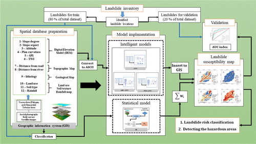
As was demonstrated previously, the main motivation of this research is to improve the efficiency of typical ANN model utilizing two potent optimization algorithms, namely artificial bee colony (ABC) and PSO. Investigating the risk of landslide occurrence in the northern part of Iran is aimed, using a statistical approach (e.g. SI) and ANN optimized with PSO (PSO-ANN), ABC (ABC-ANN). General steps of LSM producing process could be explained as follows: First, data layers from all sources were prepared. Overall, 12 landslide-conditioning (e.g. influential factors affecting the landslide) factors were derived from various sources. For achieving those, factors with basic formats (point, polygon, polyline) were converted to raster and extracted for the intended area. Similar to other studies (Wu et al. 2014; Regmi et al. 2016; Xie et al. 2017), to reveal the relationship between causative factors and landslide occurrence risk, 80% of total landslide points (i.e. 59) opted for the training process; and the remaining 20% (i.e. 15 landslides) were used to evaluate the performance of the proposed methods. Then, SI, PSO-ANN, ABC-ANN and ANN were implemented to calculate the LSVs. Eventually, the maps produced by each method were drawn in GIS and stratified in five classes of susceptibility, namely very low, low, moderate, high and very high. To assess the accuracy of the purposed predictive models, the AUC index, which is a well-known factor for such works, was calculated for the resulted maps. Figure 4 illustrates the graphical methodology of the present study.

Figure 4.  The graphical methodology of applied procedure for landslide hazard zonation.

4.1. SI method

One of the simply used methods for forecasting landslide hazard is an SI. Bivariate statistical analysis is the essence of this technique that was presented by van Westen (1997a) for LSM. According to Yesilnacar (2005), SI technique provides a proper direct mapping associated with different GIS options such as data-driven analytical ability (Pourghasemi et al. 2013b; Gao et al. 2018a, 2019). In a simple description, the importance of sub-classes of every independent factor is determined by calculating a weight, considering the distribution of the prone pixels. To do so, the number of pixels that landslide has occurred in them is divided by the entire pixels of the area. Firstly, this procedure must be performed for a specific (e.g. purposed) class, and then for the whole map. By dividing these values (Equation (3)(3) $$W_{\mathrm{SC}}=\hspace{0.17em}\text{ln}\hspace{0.17em}\left(\frac{D_{\mathrm{class}}}{D_{\mathrm{map}}}\right)=\hspace{0.17em}\text{ln}\hspace{0.17em}\left(\frac{\raisebox{1ex}{$N_{\mathrm{pix}}\left(D_i\right)$}\!\left/ \!\raisebox{-1ex}{$N_{\mathrm{pix}}\left(E_i\right)$}\right.}{\raisebox{1ex}{$\sum N_{\mathrm{pix}}\left(D_i\right)$}\!\left/ \!\raisebox{-1ex}{$\sum N_{\mathrm{pix}}\left(E_i\right)$}\right.}\right)$$(3) ), the weight for the corresponding class appears (Çevik and Topal 2003): (3) $$W_{\mathrm{SC}}=\hspace{0.17em}\text{ln}\hspace{0.17em}\left(\frac{D_{\mathrm{class}}}{D_{\mathrm{map}}}\right)=\hspace{0.17em}\text{ln}\hspace{0.17em}\left(\frac{\raisebox{1ex}{$N_{\mathrm{pix}}\left(D_i\right)$}\!\left/ \!\raisebox{-1ex}{$N_{\mathrm{pix}}\left(E_i\right)$}\right.}{\raisebox{1ex}{$\sum N_{\mathrm{pix}}\left(D_i\right)$}\!\left/ \!\raisebox{-1ex}{$\sum N_{\mathrm{pix}}\left(E_i\right)$}\right.}\right)$$(3) where${\mathrm{ }W}_{\mathrm{sc}}$ is the weight attributes to the categorical unit, $D_{\mathrm{class}}$ and $D_{\mathrm{map}}$ are is the landslide density for purposed class and entire map, respectively. Also, $N_{\mathrm{pix}}\left(D_i\right)$ indicates the number of landslides in the intended area, and $N_{\mathrm{pix}}\left(E_i\right)$ stands for the total number of pixels for purposed class. Although landslide map can be plotted by any extent of values (i.e. even with normalized values), but in this equation, natural logarithm is applied in order to produce negative and positive values of W, for less and more susceptibility rather normal situation (Van Westen 1997b; Gao et al. 2018b).

4.2. Multi-layer perceptron (MLP)

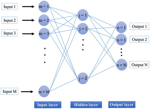
In the last two decades, the application of computational intelligence, especially ANN has raised rapidly, for solving various engineering problems. ANNs’ structure is inspired by the biological neural network, and it is a capable tool to establish non-linear equations between input(s) and output(s) of a model (Wang 2003). The facility of implementation can be mentioned as the main superiority of this method, compared to the approaches, which are based on statistical rules. The statistical distribution of the input layers and landslide events is not a determinant factor for training the ANN (Asadi et al. 2011a, 2011b; Moayedi and Rezaei 2017; Mosallanezhad and Moayedi 2017). In other words, numerical data do not need to be defined in different classes to be used by the network. MLP neural network (MLPNN) is one of the most efficient types of ANNs. As the name connotes, the MLP network is constructed from three layers, namely the input layer, hidden layer and output layer. Note that, MLP can contain more than one hidden layer, but it has been shown in various studies that one hidden layer is sufficient for modeling any complex problem (Hornik et al. 1989; Moayedi and Armaghani 2017; Moayedi 2018; Moayedi and Hayati 2018a, 2018b, 2018c; Alnaqi et al. 2019). The graphical methodology of MLP is shown in Figure 5. Each layer contains a number of ‘processing units’ called computational neurons. When the input-target pairs are received by a neuron, it commences acquiring the non-linear relationship between them. This is carried out through updating the weights and biases in each iteration. Considering the input and output vectors, the jth neuron calculates the output as follows: (4) $$O_j=F\mathrm{ }\left(\mathrm{ }\sum _{m=1}^M(I_{m\mathrm{ }}{W}_{\mathit{mj}}\right)+b_{j\mathrm{ }})$$(4) where$I$ denotes the input value, $W$ and b are the weight and bias belonging the neuron. Also, $F\mathrm{ }$is the activation function that in this study is considered to be hyperbolic tangent sigmoid (briefly Tansig). Equation (5)(5) $$\mathrm{Tansig}\left(x\right)=\frac{2}{1+e^{-2x}}-1$$(5) expresses this function: (5) $$\mathrm{Tansig}\left(x\right)=\frac{2}{1+e^{-2x}}-1$$(5)

Figure 5.  The general structure of MLP.

Moreover, in this study, the feed-forward back-propagation (FFBP) method is applied in which the initial weights and biases are adjusted in a backward path, responding to the computed error. More detail for the theory of FFBP networks can be found in Haykin (1994). Besides, the Levenberg-Marquardt training algorithm is employed for the landslide hazard approximation, due to its better performance in comparison with the conventional gradient descent (GD) techniques (Hagan and Menhaj 1994; El-Bakry 2003)

4.3. ABC algorithm

Inspired by the behaviour of natural bees Karaboga (2005) suggested the ABC algorithm. Searching the food sources (nectars) and sharing the data with other honey bees is the essence of this idea. The solution is performed by three kinds of bees, namely employed bees, onlookers and scouts. It is to be noted that onlookers and scouts are known as unemployed bees. In this approach, each possible solution is demonstrated by the position of a food source; and its efficiency (fitness) is evaluated by the amount of nectar in the proposed food source. Since every employed bee belongs to one food source, these two parameters receive the same values. Like other optimization algorithms, ABC commences with an initialization phase and then, the main search cycle is executed, and it until an acceptable performance rate or the maximum iteration is met. During the initialization phase, an initial population is constructed with a random distribution, and after that, the solution is subjected to repeat the search process of the employed, onlooker and scout bees. The employed bees seek new food sources (V_ij) with more nectar within the vicinity of the recognized food source (X_ij). Then, they examine the quality of the discovered source. The parameters are defined by the following formula: (6) $$\mathit{Vij}\mathrm{ }=\mathrm{ }\mathit{Xij}\mathrm{ }+\mathrm{ }\mathit{rand}\mathrm{ }[0,1]\mathrm{ }.\mathrm{ }(\mathit{Xij}\mathrm{ }–\mathrm{ }\mathit{Xmj})$$(6) where$\mathrm{ }i\mathrm{ }$indicated the randomly picked parameter index ($i\ne m$). Also, $V_{\mathit{ij}}$ and $X_{\mathit{mj}}$ stand for the new and determined food sources, respectively. After obtaining fresh food source ($V_{\mathit{ij}}$), the best source is chosen between $V_{\mathit{ij}}$ and $X_{\mathit{ij}}$X_ij, with respect to the corresponding fitness.

Onlooker bees must choose their food source considering the information about food sources is shared by employed bees. This selection depends on the probability values ($P_i$) that is given by the calculated fitness values. $P_i$ is defined by the following equation: (7) $$P_i=\frac{f_i \left(X_i\right)}{{\sum }_{i=1}^z{f}_i \left(X_i\right)}$$(7) where $f_i\mathrm{ }$describes the fitness of the food source. Following this, the algorithm updates the food sources by recruiting more onlooker individuals. In the ABC programming, an ‘abandonment criteria’ is determined which is representative of the employed bees that their solution cannot be enhanced during a fixed number of trials. These bees are known as scouts, and their solution is deserted. In addition, they begin to look for new random solutions (Karaboga et al. 2007). Figure 6(a) illustrates the flowchart of the ABC algorithm implementation.

Figure 6. General mechanism of (a) ABC algorithm and (b) ABC-ANN method.

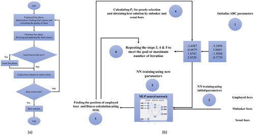
4.4. Combination of ANN and ABC

Figure 6(b) exhibits the learning process of ABC-ANN algorithm. During this technique, it has been aimed to generate the optimum values for interconnection weights and biases of ANN. In this way, the ANN network is developed by some initial parameters. In the following, the ABC relations (i.e. employed, onlookers and scout bees) discover and evaluate various positions (food sources) and attempt to replace the ANN initial parameters with the most appropriate alternatives. This procedure is carried out by defining an objective function (here mean absolute error (MSE)) to achieve the best solution (Sarangi et al. 2014). More details about this technique can be found in Nandy et al. (2012).

4.5. PSO algorithm

PSO is a powerful metaheuristic algorithm that is first designed by Eberhart and Kennedy (1995). The higher learning speed and requiring less memory are the main advantages of this technique, compared to other optimization algorithms (e.g. GA and imperialist competition algorithm (Moayedi et al. 2018). During the PSO implementation, two parameters of g_best (the best global positions) and p_best (the most proper personal) are found by the particle activities. Equations (8)(8) $$X_2= X_1+ V_2$$(8) and (9)(9) $$V_2=\omega \times V_1+C_1\times r_1\left(p_{\text{best}}- X_1\right)+C_2\times r_2\left(g_{\text{best}}- X_1\right)$$(9) formulate the position and velocity of the particles, respectively. (8) $$X_2= X_1+ V_2$$(8) (9) $$V_2=\omega \times V_1+C_1\times r_1\left(p_{\text{best}}- X_1\right)+C_2\times r_2\left(g_{\text{best}}- X_1\right)$$(9) in which X₁ and X₂ are the current and new positions of the particles, and V₁ and V₂ denote the current and new velocities of the particles, respectively. Also, C₁ and C₂ symbolize two constant and user-defined acceleration variables, r₁ and r₂ stand for random values that can be determined as (0,1), and ω indicates the inertia weight. Moreover, Figure 7(a) shows a graphical description from the PSO performance.

Figure 7. General mechanism of (a) PSO algorithm and (b) PSO-ANN method.

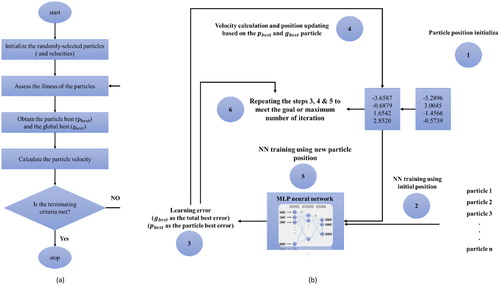
4.6. Combination of ANN with PSO

Figure 7(b) depicts the learning process of the hybrid PSO-ANN model. Similar to the ABC algorithm, PSO gets started with an initialization phase, which selects the ANN connection parameters (particle’s positions) randomly. The convergence of the trained network is checked recursively by defining an objective function (e.g. MSE). The optimization continues by updating the $\overrightarrow{g_{\mathrm{best}}}$ and $\overrightarrow{p_{\mathrm{best}}}$ values. As a maxim, PSO aims to minimize the MSE criterion, until one of the defined stopping conditions is met. The outcome of this procedure is to extract the best solution by adjusting the weights and biases of the proposed ANN. Further information about this model is well-detailed in various studies (Chen et al. 2017a).

5. Results and discussion

5.1. Statistical index

The landslide distribution map and its effective factor layers were prepared in ArcGIS 10.2 software. Classifying the values of each factor was done based on the authors’ experience and previous studies (Regmi et al. 2014; Moayedi et al. 2018). The landslide inventory dataset divided into 2 classes indicating landslide (1) and no-landslide (0) occurrence. During the SI model, independent layers have been crossed by landslide raster one by one to acquire the spatial relationship between them. The attribute table of the resulting layer contains the distribution of landslide in each sub-class (see Table 1). As is clearly described in Table 1, no slope failure has been reported for altitude more than 600-m. Additionally, almost all of the landslide-prone pixels are in the range of 0°–10° for the slope degree conditioning factor. This is while a higher frequency of landslides is expected for the steep slopes, due to the lower shear stresses associated with high gradients. As for independent rainfall factor, the study area is located in the northern part of Iran, which is known for heavy precipitations. As is known, regular precipitations cause loss of shear strength of the soil slopes. It was observed that the distribution of landslides is directly proportional to the annual amount of rainfall. Approximately one-third (33.87%) of pixels that indicate the landslide occurrence is classified by the precipitation more than 524 mm/year. In the case of the lithology of the study area, almost entire landslides (99.71% of prone cells) have been observed in the fifth group of rocks, namely swamp sedimentary rocks. Due to the proximity of the linear phenomena (i.e. roads and rivers) to each other, a nearly equal contribution of landslides is obtained for them. In the case of distance from the road, for example, many mass movements have been triggered by road cutting operations (Nefeslioglu et al. 2008). Also, the presence of the streams affects the likelihood of the slope failure through changing the drainage rate, air humidity and erosion susceptibility of the study area (Pourghasemi et al. 2013a; Hu et al., 2018). In this regard, the distance range of 0–100 m contains approximately half of (45.92% and 55.41%, respectively, for roads and rivers) landslide representative cells. In the following, the computation process of the SI method carried out in Excel 2010 software.

Table 1.  The spatial relationship between the landslide and its causative factors.

Factor	Classes	No. of pixels	Percentage of domain	No. of prone pixels	Percentage of prone pixels
Slope degree	0–10°	1,292,418	79.23	15,435	99.31
	10–20°	293,940	18.02	108	0.69
	20–30°	40,950	2.51	0	0.00
	30–40°	3807	0.23	0	0.00
	>40°	63	0.00	0	0.00
Slope aspect	North (0–22.5°)	40,158	2.46	0	0.00
	North-East	55,953	3.43	225	1.45
	East	58,023	3.56	126	0.81
	South-East	89,091	5.46	513	3.30
	South	103,032	6.32	531	3.42
	South-West	100,998	6.19	1305	8.40
	West	112,365	6.89	549	3.53
	North-West	228,420	14.00	657	4.23
	North (337.5–360°)	71,658	4.39	270	1.74
	Flat	771,480	47.30	11,367	73.13
Elevation (m)	200–300	348,750	21.38	6228	40.07
	300–450	620,343	38.03	8685	55.88
	450–600	593,946	36.41	630	4.05
	600–750	60,102	3.68	0	0.00
	>750	8037	0.49	0	0.00
Plan Curvature	Concave (–4 – –0.0 01)	14,958	0.92	0	0
	Flat (–0.001–0.001)	1,601,955	98.21	15,543	100
	Convex (0.001–4)	14,265	0.87	0	0
Lithology	Group 1	37,710	2.31	45	0.29
	Group 2	11,898	0.73	0	0.00
	Group 3	51,201	3.14	0	0.00
	Group 4	4752	0.29	0	0.00
	Group 5	1,525,617	93.53	15,498	99.71
Soil Type	Group 1	97,506	5.98	306	1.97
	Group 2	172,800	10.59	0	0.00
	Group 3	1,360,872	83.43	15,237	98.03
Land use	A	5967	0.37	873	5.62
	B	260,253	15.95	3762	24.20
	C	6732	0.41	27	0.17
	D	48,825	2.99	0	0.00
	E	144,612	8.87	1359	8.74
	F	256,266	15.71	45	0.29
	G	22,248	1.36	0	0.00
	H	44,163	2.71	0	0.00
	I	347,481	21.30	5076	32.66
	J	213,075	13.06	2043	13.14
	K	155,880	9.56	612	3.94
	L	123,408	7.57	1017	6.54
	M	2268	0.14	729	4.69
Distance from road (m)	0–100	100,872	6.18	7137	45.92
	100–200	85,446	5.24	3537	22.76
	200–300	90,909	5.57	1611	10.36
	300–400	77,940	4.78	747	4.81
	>400	1,276,011	78.23	2511	16.16
Distance from river (m)	0–100	120,582	7.39	8613	55.41
	100–200	100,062	6.13	3663	23.57
	200–300	105,840	6.49	1035	6.66
	300–400	87,003	5.33	540	3.47
	>400	1,217,691	74.65	1692	10.89
Rainfall (mm/year)	476–491	145,440	8.92	1449	9.32
	491–503	228,321	14.00	3429	22.06
	503–514	313,902	19.24	2484	15.98
	514–524	380,691	23.34	2916	18.76
	524–535	562,824	34.50	5265	33.87
SPI	0–10	1,568,061	96.13	14,940	96.12
	10–20	22,194	1.36	108	0.69
	20–30	8892	0.55	9	0.06
	30–40	5958	0.37	162	1.04
	>40	26,073	1.60	324	2.08
TWI	–6––2	114,642	7.03	495	3.18
	–2–3	494,343	30.31	1206	7.76
	3–6	333,207	20.43	2277	14.65
	6–10	543,942	33.35	7866	50.61
	>10	145,044	8.89	3699	23.80

5.2. Artificial intelligence models

The second part of the current study aimed to produce the LSM based on the purposed ANN and hybrid (ABC-ANN and PSO-ANN) method. The required dataset for developing the mentioned networks was derived through converting GIS spatial database from raster to ASCII format. In fact, every raster contains special values, which are assigned to a special pixel. A landslide distribution map was used to compose target data and 12 inputs (e.g. elevation, slope degree, lithology, rainfall, SPI, TWI, distance to road, distance to river, land use, slope aspect, soil type and plan curvature) were inserted to train the predictive network models and produce the LSV as an output. For nominal data (lithology, for instance), the title of each class is altered with continuous values equal to their group number (shown in Figure 3) to become acceptable for the network. During the implementation of artificial intelligence tools, at least two stages of data are needed. The first part, which called the training stage, is the chief part of the dataset, and are used to educate the system. Learning process includes adjusting inter-layer weights and biases to reduce the error in each iteration. The trained network must be evaluated by the second stage called the test phase. Test data are different from another phase, and the performance accuracy of the trained network is distinguished by them. Dividing the dataset was done by 80% and 20% ratio (59 and 15 landslide cases), respectively for the train and test phase. Finding the appropriate network architecture is a fundamental step in the field of soft computing utilization. To this subject, an extensive trial and error process was carried out for ANN, ABC-ANN and PSO-ANN networks. The MSE index was used to evaluate the performance of modes. When the optimum structure is determined, the optimized weights and biases were arranged to compute the outputs of each predictive model.

5.2.1. Artificial neural network

To find the best ANN architecture, an MLP network was tested by 10 different numbers of neurons in its unique hidden layer (i.e. hidden neurons). Figure 8 denotes the result of this procedure.

Figure 8. Sensitivity analysis for ANN based on the number of hidden neurons.

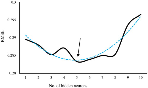
As is clearly seen, the ANN with at five neurons in the hidden layer could present more precise execution (i.e. the lowest error). Therefore, the optimum ANN structure could be defined as 12 × 5 × 1 indicating the MLP structure with 12, 5 and 1 neurons in its input, hidden and output layers, respectively. In addition, the weights and biases extracted from ANN are presented in Table 2.

Table 2. Weight and biases of the ANN model.

Neuron (i)	i
	LSV = –0.0047 × Z1 – 0.1870 × Z2 – 0.1439 × Z3 – 0.0145 × Z4 – 0.1459 × Z5 – 1.1577
	Zi = Tansig (Wi1 × A + Wi2 × B + … + Wi12 × L + bi)
	Wi1	Wi2	Wi3	Wi4	Wi5	Wi6	Wi7	Wi8	Wi9	Wi10	Wi11	Wi12	bi
1	–0.4559	–0.3531	0.1034	0.4904	0.5098	–0.6757	–0.1303	0.4670	–0.5694	–0.5553	–0.3443	0.4398	1.6856
2	0.9809	–0.0107	–0.1714	0.1445	0.4505	0.0195	–0.6466	0.1435	–0.1218	–0.7780	0.3958	–0.2329	–0.5345
3	–0.1577	0.2106	0.1482	–0.1720	–0.8059	0.3104	0.6322	0.0982	0.6408	0.4697	0.0248	1.0436	0.143
4	0.6646	–0.1131	–0.1888	–0.0024	0.6835	0.5731	0.7293	0.8883	–0.0716	0.5503	0.2718	–0.3435	0.7654
5	–0.5450	–0.1343	0.8396	0.5029	–0.2736	–0.1200	–0.1491	–0.5532	–0.3939	0.1899	–0.3579	–0.8073	–1.4422

5.2.2. ABC-ANN model

In order to amend the defects of BP learning method in ANN, an ABC optimization algorithm is applied. This algorithm attempts to adjust the ANN parameters. This is noteworthy that this work repeats until the lowest error is reached. To find the most suitable ABC architecture, different colony sizes were tested within 1000 iterations. As Figure 9 shows, colony size was considered to vary from 50 to 500 with 50 intervals to assess the impact of changes in the number of bees. It must be mentioned that no significant change in MSE values is observed after the thousandth cycle. According to Koopialipoor et al. (2018), the tendency of bees to convene in the place with the best response is the main cause that this occurs. In this respect, the least MSE acquired for ABC network with colony size equals to 150. The produced landslide hazard map and ABC-ANN derived optimal weights and biases are presented in Figure 11(c) and Table 3, respectively.

Figure 9. Sensitivity analysis for ABC-ANN based on colony size.

Table 3. Optimized weight and biases of the ABC-ANN model.

Neuron (i)	LSV = –0.0001 × Z1 + 0.0209 × Z2 + 0.0054 × Z3 + 0.0085 × Z4 – 0.1678 × Z5 – 0.8261
	Zi = Tansig (Wi1 × A + Wi2 × B + … + Wi12 × L + bi)
	Wi1	Wi2	Wi3	Wi4	Wi5	Wi6	Wi7	Wi8	Wi9	Wi10	Wi11	Wi12	bi
1	3.2219	5.1953	–51.9518	–75.6243	–6.8825	365.7876	–0.5138	–133.7595	–0.7071	–3.0083	–27.4672	–8.8390	192.7512
2	–1022.4356	–79.0813	–85.6538	36.9012	–24.4347	–29.3689	374.2896	–26.1480	–7.6598	3.7417	–12.1546	0.2060	–12.5510
3	11.9548	30.3340	80.5551	–7.7851	–100.3677	–51.5862	8.0825	83.1883	–12.0480	12.7368	–18.7648	–2.0783	–20.6393
4	126.5222	0.1142	–25.1545	–13.8558	–655.3529	68.3088	12.0814	–38.5672	8.8144	–48.6130	–77.2456	46.2577	13.1375
5	98.3364	21.7059	18.0298	–2.6837	–797.7548	–55.2426	0.2987	13.4053	886.3462	23.5468	130.8857	75.4644	168.7963

5.2.3. PSO-ANN model

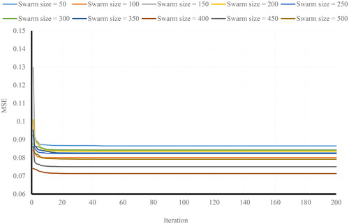
Considering the previous explanation about the PSO algorithm, apart from the number of iterations, several characteristics such as swarm size, inertia weight and coefficient of velocity equation also affect the performance of an applied PSO algorithm. In this subject and due to the variety of determinant factors, the authors decided to use similar values that have been successfully assigned to previous PSO works. The coefficient of velocity equation and inertia weight were considered to receive the values 2 and 0.25, respectively (Clerc and Kennedy 2002). In the next step, similar to ABC-ANN, a trial and error process was carried out to find the proper swarm size. Ten different number of swarms (from 50 to 500 with 50 intervals) were employed, and the MSE was calculated. Based on the obtained error (Figure 10), the best model was found to be constructed from 400 swarms. PSO-ANN approximation of LSVs has been illustrated in Figure 11(d). Furthermore, ANN parameters optimized by the PSO evolutionary algorithm are featured in Table 4.

Table 4. Optimized weight and biases of the PSO-ANN model.

Neuron (i)	LSV = –0.0275 × Z1 + 0.0951 × Z2 + 0.0147 × Z3 + 0.1397 × Z4 + 0.5515 × Z5 – 0.6988
	Zi = Tansig (Wi1 × A + Wi2 × B + … + Wi12 × L + bi)
	Wi1	Wi2	Wi3	Wi4	Wi5	Wi6	Wi7	Wi8	Wi9	Wi10	Wi11	Wi12	bi
1	0.1016	–0.3819	0.5902	0.3872	0.4509	–0.2766	–0.4612	–0.0039	–0.0252	0.4933	–0.5502	0.0117	–0.3565
2	–0.6568	–0.3073	–0.1829	–0.1773	0.0377	–0.4657	0.0109	–0.7324	0.4008	0.0306	0.2257	0.5338	0.0009
3	0.1800	0.3027	0.5275	–0.7473	0.1486	–0.2882	–0.3661	0.5142	–0.1553	0.3940	–0.2452	–0.2334	0.3769
4	0.0142	–0.3506	–0.3637	0.6541	–0.6400	–0.2534	–0.2468	–0.6497	0.5182	–0.1110	–0.2621	–0.2952	0.1199
5	–0.0246	–0.3065	0.0827	–0.1199	0.1337	0.2980	0.0844	0.3235	–0.6117	0.1419	–0.3275	–0.2340	–0.8339

Figure 10. Sensitivity analysis for PSO-ANN based on swarm size.

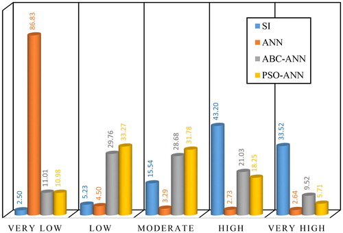
All developed LSMs (i.e. for SI, ANN, ABC-ANN, and PSO-ANN models) were depicted into five susceptibility classes with respect to natural break classification (Xu et al. 2012). The results represent an acceptable performance rate for all used techniques. According to Figure 11(a–d), the main landslide distribution path, showing the location of test and train landslide has been correctly categorized as dangerous areas (i.e. High and Very high hazard classes) by all four models. In addition, the main discernible distinction between the above maps refers to the ANN responds. As is clearly observed, the majority of ANN map is classified as safe areas. In contrast, the statistical method shows a more conservative prediction. For more details, the percentage of the pixels occupied by each susceptibility category is illustrated in Figure 12 for all employed models. According to this column chart, the majority of the area (86.83%) is identified by “Very low” susceptibility class by ANN. In addition, ABC-ANN and PSO-ANN methods exhibit an almost equivalent approximation, particularly for the first four hazard groups (Figure 12). Moreover, a total of 76.72%, 23.96%, 30.55% and 5.37% of the study area were found to be exposed by significant landslide risk (High and Very high susceptibility classes), respectively by SI, PSO-ANN, ABC-ANN, and ANN predictive models.

Figure 11. A view of landslide hazard maps developed in GIS model (a) SI, (b) ANN, (c) ABC-ANN and (b) PSO-ANN estimation of LSVs.

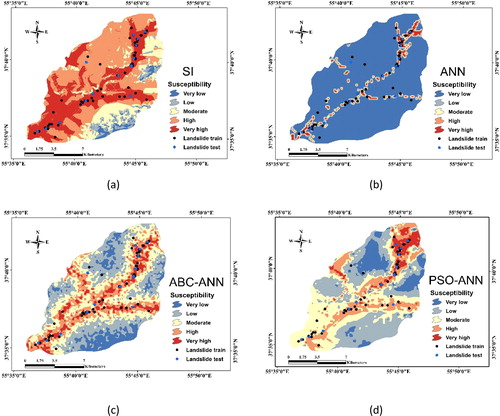
Figure 12. Column chart based on the percentage of landslide hazard classes.

In the following, the AUC index was used to evaluate the prediction accuracy of landslide predictive models (Pradhan and Lee 2010). Note that, the testing landslides (i.e. landslide validation) were considered here to evaluate the competency of each model. To do so, SPSS software was used to draw the receiving operating characteristic (ROC) curve. This diagram is available in Figure 13, indicating the true positive rate (on the vertical axis) against the false positive rate (on the horizontal axis) of assessment.

Figure 13. The ROC diagram, obtained for SI, ANN, ABC-ANN, and PSO-ANN models.

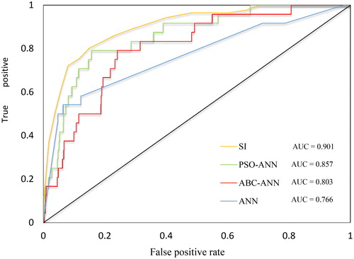
This is noteworthy that AUC can vary from 0.5 to 1 so that 1 indicates an ideal performance and adversely, a casual prediction is determined by 0.5. Referring to the calculated AUC values (which are 0.901, 0.857, 0.803 and 0.766 respectively for SI, PSO-ANN, ABC-ANN, and ANN), it can be concluded that SI with 90.1% accuracy, has shown most reliability for landslide susceptibility modelling in this study. About the artificial intelligent methods, it is concluded that applying the optimization algorithms including ABC and PSO can lead to improving the performance of the ANN model. Along with this, the accuracy rate of 85.7% reveals the superiority of PSO-ANN comparing with ABC_ANN (80.3%) and ANN (76.6%) approaches. In summary, the results of this study suggest that LSM for the purposed study area is viable. In addition, authors believe that the resulted maps could be helpful for urban land use planning and engineers in Golestan province.

6. Conclusion and remarks

Recent years have witnessed broad use of various soft computing approaches for analyzing the landslide hazard worldwide. In this paper, we assessed the feasibility and efficacy of ABC and PSO for landslide susceptibility zonation. To do so, the mentioned evolutionary algorithms were synthesized with an ANN to enhance its performance. The SI method was also implemented. To generate a reliable LSM, 12 of geological and hydrological effective factors, namely elevation, slope degree, lithology, rainfall, SPI, TWI, distance to road, distance to the river, land use, slope aspect, soil type and plan curvature were used as independent variables. Based on the results, the following conclusions were obtained in this study:

• Referring to the calculated AUCs of 0.901, 0.857, 0.803 and 0.766, respectively for SI, PSO-ANN, ABC-ANN and ANN, all applied approaches exhibited a satisfying performance.

• The efficiency of the typical ANN was effectively enhanced by applying PAO and ABC metaheuristic algorithms.

• From comparison viewpoint, SI model (90.1% accuracy) presented the most accurate prediction, followed by PSO-ANN (85.7% accuracy), ABC-ANN (80.3% accuracy) and ANN (76.6% accuracy) models.

• According to the achieved landslide hazard maps, a total of 76.72%, 23.96%, 30.55% and 5.37% of the study area were found to be exposed by high landslide risk, respectively by SI, PSO-ANN, ABC-ANN and ANN.

Finally, the results of the current study are suggested to be used for decision makers and land use planning in the study area.

Disclosure statement

No potential conflict of interest was reported by the authors.

Additional information

Funding

This research was supported by Ton Duc Thang University (Vietnam) and Duy Tan University (Vietnam).

References

- Alnaqi AA, Moayedi H, Shahsavar A, Nguyen TK. 2019. Prediction of energetic performance of a building integrated photovoltaic/thermal system thorough artificial neural network and hybrid particle swarm optimization models. Energy Conv Manag. 183:137–148.
- Althuwaynee OF, Pradhan B, Park H-J, Lee JH. 2014. A novel ensemble bivariate statistical evidential belief function with knowledge-based analytical hierarchy process and multivariate statistical logistic regression for landslide susceptibility mapping. Catena. 114:21–36.
- Arora MK, Das Gupta AS, Gupta RP. 2004. An artificial neural network approach for landslide hazard zonation in the Bhagirathi (Ganga) Valley, Himalayas. Int J Remote Sens. 25(3):559–572.
- Asadi A, Moayedi H, Huat BBK, Boroujeni FZ, Parsaie A, Sojoudi S. 2011a. Prediction of zeta potential for tropical peat in the presence of different cations using artificial neural networks. Int J Electrochem Sci. 6:1146–1158.
- Asadi A, Moayedi H, Huat BBK, Parsaie A, Taha MR. 2011b. Artificial neural networks approach for electrochemical resistivity of highly organic soil. Int J Electrochem Sci. 6:1135–1145.
- Baeza C, Corominas J. 2001. Assessment of shallow landslide susceptibility by means of multivariate statistical techniques. Earth Surf Process Landforms. 26(12):1251–1263.
- Balamurugan G, Ramesh V, Touthang M. 2016. Landslide susceptibility zonation mapping using frequency ratio and fuzzy gamma operator models in part of NH-39, Manipur, India. Nat Hazards. 84(1):465–488.
- Bui DT, Tuan TA, Hoang N-D, Thanh NQ, Nguyen DB, Van Liem N, Pradhan B. 2017. Spatial prediction of rainfall-induced landslides for the Lao Cai area (Vietnam) using a hybrid intelligent approach of least squares support vector machines inference model and artificial bee colony optimization. Landslides. 14:447–458.
- Çevik E, Topal T. 2003. GIS-based landslide susceptibility mapping for a problematic segment of the natural gas pipeline, Hendek (Turkey). Environ Geol. 44(8):949–962.
- Chaytor JD, Geist EL, Paull CK, Caress DW, Gwiazda R, Fucugauchi JU, Vieyra MR. 2016. Source characterization and tsunami modeling of submarine landslides along the yucatan shelf/campeche escarpment, Southern Gulf of Mexico. Pure Appl Geophys. 173(12):4101–4116.
- Chen W, Li W, Chai H, Hou E, Li X, Ding X. 2016. GIS-based landslide susceptibility mapping using analytical hierarchy process (AHP) and certainty factor (CF) models for the Baozhong region of Baoji City, China. Environ Earth Sci. 75:63–76..
- Chen W, Li W, Hou E, Bai H, Chai H, Wang D, Cui X, Wang Q. 2015. Application of frequency ratio, statistical index, and index of entropy models and their comparison in landslide susceptibility mapping for the Baozhong Region of Baoji, China. Arab J Geosci. 8(4):1829–1841.
- Chen W, Panahi M, Pourghasemi HR. 2017a. Performance evaluation of GIS-based new ensemble data mining techniques of adaptive neuro-fuzzy inference system (ANFIS) with genetic algorithm (GA), differential evolution (DE), and particle swarm optimization (PSO) for landslide spatial modelling. Catena. 157:310–324.
- Chen W, Panahi M, Tsangaratos P, Shahabi H, Ilia I, Panahi S, Li S, Jaafari A, Ahmad BB. 2019. Applying population-based evolutionary algorithms and a neuro-fuzzy system for modeling landslide susceptibility. Catena. 172:212–231.
- Chen W, Pourghasemi HR, Panahi M, Kornejady A, Wang J, Xie X, Cao S. 2017b. Spatial prediction of landslide susceptibility using an adaptive neuro-fuzzy inference system combined with frequency ratio, generalized additive model, and support vector machine techniques. Geomorphology. 297:69–85.
- Cheng M-Y, Hoang N-D. 2015. Typhoon-induced slope collapse assessment using a novel bee colony optimized support vector classifier. Nat Hazards. 78(3):1961–1978.
- Clerc M, Kennedy J. 2002. The particle swarm-explosion, stability, and convergence in a multidimensional complex space. IEEE Trans Evol Computat. 6(1):58–73.
- Dong Y, Wang D, Randolph MF. 2017. Runout of submarine landslide simulated with material point method. Proceedings of the 1st International Conference on the Material Point Method. Amsterdam: Elsevier Science Bv. p. 357–364.
- Eberhart R, Kennedy J. 1995. A new optimizer using particle swarm theory. Proceedings of the Micro Machine and Human Science, 1995. MHS'95. Proceedings of the Sixth International Symposium on IEEE: Nagoya, Japan, Japan.
- El-Bakry MY. 2003. Feedforward neural networks modelling for K–P interactions. Chaos Solitons Fractals. 18:995–1000.
- Ercanoglu M, Gokceoglu C. 2002. Assessment of landslide susceptibility for a landslide-prone area (north of Yenice, NW Turkey) by fuzzy approach. Environ. Geol. 41:720–730.
- Ercanoglu M, Gokceoglu C. 2004. Use of fuzzy relations to produce landslide susceptibility map of a landslide-prone area (West Black Sea Region, Turkey). Eng Geol. 75(3–4):229–250.
- Farrokhzad F, Barari A, Ibsen LB, Choobbasti AJ. 2011. Predicting subsurface soil layering and landslide risk with Artificial Neural Networks: a case study from Iran. Geol Carpath. 62(5):477–485.
- Gao W, Dimitrov D, Abdo H. 2018a. Tight independent set neighbourhood union condition for fractional critical deleted graphs and ID deleted graphs. Discr Cont Dyn Syst-S. 123–144.
- Gao W, Guirao JLG, Abdel-Aty M, Xi W. 2019. An independent set degree condition for fractional critical deleted graphs. Discr Cont Dyn Syst. 12:877–886.
- Gao W, Guirao JLG, Basavanagoud B, Wu J. 2018b. Partial multi-dividing ontology learning algorithm. Inf Sci. 467:35–58.
- Gao W, Wang W, Dimitrov D, Wang Y. 2018c. Nano properties analysis via fourth multiplicative ABC indicator calculating. Arab J Chem. 11(6):793–801.
- Gao W, Wu H, Siddiqui MK, Baig AQ. 2018. Study of biological networks using graph theory. Saudi J Biol Sci. 25(6):1212–1219.
- Hagan MT, Menhaj MB. 1994. Training feedforward networks with the Marquardt algorithm. IEEE Trans Neural Netw. 5(6):989–993.
- Haykin S. 1994. Neural networks: a comprehensive foundation. Upper Saddle River, New Jersey (NJ): Prentice Hall PTR.
- Hong H, Liu J, Zhu A-X, Shahabi H, Pham BT, Chen W, Pradhan B, Bui DT. 2017. A novel hybrid integration model using support vector machines and random subspace for weather-triggered landslide susceptibility assessment in the Wuning area (China). Environ Earth Sci. 76:652.
- Hong HY, Naghibi SA, Pourghasemi HR, Pradhan B. 2016. GIS-based landslide spatial modeling in Ganzhou City, China. Arab J Geosci. 9:26.
- Hoque Mozumder, M M, Shamsuzzaman, M M, Rashed-Un-Nabi, M, Karim, E. 2018. Social-ecological dynamics of the small scale fisheries in Sundarban Mangrove Forest, Bangladesh. Aquaculture and Fisheries. 3(1):38–49. doi:10.1016/j.aaf.2017.12.002.
- Hornik K, Stinchcombe M, White H. 1989. Multilayer feedforward networks are universal approximators. Neural Netw. 2(5):359–366.
- Hu, S, Guan, X, Guo, M, Wang, J. 2018. Environmental load of solid wood floor production from larch grown at different planting densities based on a life cycle assessment. J FOR Res. 29(5):1443–1448. doi:10.1007/s11676-017-0529-x.
- Karaboga D. 2005. An idea based on honey bee swarm for numerical optimization. Turkey: Erciyes University; Technical report-TR06.
- Karaboga D, Akay B, Ozturk C. 2007. Artificial bee colony (ABC) optimization algorithm for training feed-forward neural networks. Proceedings of the International conference on modeling decisions for artificial intelligence; Springer.
- Koopialipoor M, Armaghani DJ, Hedayat A, Marto A, Gordan B. 2018. Applying various hybrid intelligent systems to evaluate and predict slope stability under static and dynamic conditions. Soft Comput. 1–17.
- Lee S, Ryu J-H, Won J-S, Park H-J. 2004. Determination and application of the weights for landslide susceptibility mapping using an artificial neural network. Eng. Geol. 71(3–4):289–302.
- Lian C, Zeng ZG, Yao W, Tang HM. 2013. Displacement prediction model of landslide based on a modified ensemble empirical mode decomposition and extreme learning machine. Nat Hazards. 66(2):759–771. Mar
- Meng QK, Miao F, Zhen J, Wang XY, Wang A, Peng Y, Fan Q. 2016. GIS-based landslide susceptibility mapping with logistic regression, analytical hierarchy process, and combined fuzzy and support vector machine methods: a case study from Wolong Giant Panda Natural Reserve, China. Bull Eng Geol Environ. 75(3):923–944.
- Moayedi H. 2018. Optimization of ANFIS with GA and PSO estimating α in driven shafts. Eng Comput. 35:1–12.
- Moayedi H, Armaghani DJ. 2017. Optimizing an ANN model with ICA for estimating bearing capacity of driven pile in cohesionless soil. Eng Comput. 1–10.
- Moayedi H, Hayati S. 2018a. Applicability of a CPT-based neural network solution in predicting load-settlement responses of bored pile. Int J Geomech. 18.
- Moayedi H, Hayati S. 2018b. Artificial intelligence design charts for predicting friction capacity of driven pile in clay. Neural Comput Appl. 31:1–17. https://doi.org/10.1007/s00521-018-3555-5.
- Moayedi H, Hayati S. 2018c. Modelling and optimization of ultimate bearing capacity of strip footing near a slope by soft computing methods. Appl Soft Comput. 66:208–219.
- Moayedi H, Huat BBK, Mohammad Ali TA, Asadi A, Moayedi F, Mokhberi M. 2011. Preventing landslides in times of rainfall: case study and FEM analyses. Disaster Prev Manag. 20(2):115–124.
- Moayedi H, Mehrabi M, Mosallanezhad M, Rashid ASA, Pradhan B. 2018. Modification of landslide susceptibility mapping using optimized PSO-ANN technique. Eng Comput. 35(2):1–18. DOI: 10.1007/s00366-018-0644-0.
- Moayedi H, Rezaei A. 2017. An artificial neural network approach for under-reamed piles subjected to uplift forces in dry sand. Neural Comput Appl. 1–10.
- Mokoena, B T, Musakwa, W. 2018. Mobile GIS occupancy audit of Ulana informal settlement in Ekurhuleni municipality, South Africa. Geo-Spatial Information Science. 21(4):322–330. doi:10.1080/10095020.2018.1519349.
- Moore ID, Grayson RB, Ladson AR. 1991. Digital terrain modelling: a review of hydrological, geomorphological, and biological applications. Hydrol Process. 5(1):3–30.
- Mosallanezhad M, Moayedi H. 2017. Developing hybrid artificial neural network model for predicting uplift resistance of screw piles. Arab J Geosci. 10:10. Nov
- Nandy S, Sarkar PP, Das A. 2012. Training a feed-forward neural network with artificial bee colony based backpropagation method. 1209:2548. arXiv preprint arXiv
- Nefeslioglu HA, Gokceoglu C, Sonmez H. 2008. An assessment on the use of logistic regression and artificial neural networks with different sampling strategies for the preparation of landslide susceptibility maps. Eng Geol. 97(3–4):171–191.
- Oh H-J, Pradhan B. 2011. Application of a neuro-fuzzy model to landslide-susceptibility mapping for shallow landslides in a tropical hilly area. Comput Geosci. 37(9):1264–1276.
- Parsons T, Geist EL, Ryan HF, Lee HJ, Haeussler PJ, Lynett P, Hart PE, Sliter R, Roland E. 2014. Source and progression of a submarine landslide and tsunami: the 1964 Great Alaska earthquake at Valdez. J Geophys Res Solid Earth. 119(11):8502–8516. Nov
- Pourghasemi HR, Beheshtirad M, Pradhan B. 2016. A comparative assessment of prediction capabilities of modified analytical hierarchy process (M-AHP) and Mamdani fuzzy logic models using Netcad-GIS for forest fire susceptibility mapping. Geomat Nat Hazards Risk. 7(2):861–885.
- Pourghasemi HR, Jirandeh AG, Pradhan B, Xu C, Gokceoglu C. 2013a. Landslide susceptibility mapping using support vector machine and GIS at the Golestan Province, Iran. J Earth Syst Sci. 122(2):349–369.
- Pourghasemi HR, Mohammady M, Pradhan B. 2012a. Landslide susceptibility mapping using index of entropy and conditional probability models in GIS: Safarood Basin, Iran. Catena. 97:71–84.
- Pourghasemi HR, Moradi HR, Aghda SF. 2013b. Landslide susceptibility mapping by binary logistic regression, analytical hierarchy process, and statistical index models and assessment of their performances. Nat Hazards. 69(1):749–779.
- Pourghasemi HR, Pradhan B, Gokceoglu C. 2012b. Application of fuzzy logic and analytical hierarchy process (AHP) to landslide susceptibility mapping at Haraz watershed, Iran. Nat Hazards. 63(2):965–996.
- Pradhan B. 2010. Landslide Susceptibility mapping of a catchment area using frequency ratio, fuzzy logic and multivariate logistic regression approaches. J Indian Soc Remote Sens. 38(2):301–320.
- Pradhan B, Lee S. 2010. Regional landslide susceptibility analysis using back-propagation neural network model at Cameron Highland, Malaysia. Landslides. 7(1):13–30.
- Regmi AD, Devkota KC, Yoshida K, Pradhan B, Pourghasemi HR, Kumamoto T, Akgun A. 2014. Application of frequency ratio, statistical index, and weights-of-evidence models and their comparison in landslide susceptibility mapping in Central Nepal Himalaya. Arab J Geosci. 7(2):725–742.
- Regmi AD, Dhital MR, Zhang J-Q, Su L-J, Chen X-Q. 2016. Landslide susceptibility assessment of the region affected by the 25 April 2015 Gorkha earthquake of Nepal. J Mt Sci. 13(11):1941–1957.
- Sarangi PP, Sahu A, Panda M. 2014. Training a feed-forward neural network using artificial bee colony with back-propagation algorithm. Intell Comput Network Inf. 243:511–519.
- Shahri AA. 2016. An optimized artificial neural network structure to predict clay sensitivity in a high landslide prone area using piezocone penetration test (CPTu) data: a case study in Southwest of Sweden. Geotech Geol Eng. 34:745–758.
- Vakhshoori V, Zare M. 2016. Landslide susceptibility mapping by comparing weight of evidence, fuzzy logic, and frequency ratio methods. Geomat Nat Hazards Risk. 7(5):1731–1752.
- Van Westen C. 1997a. Statistical landslide hazard analysis. ILWIS 2.1 for windows application guide. Enshede, The Netherlands: ITC Publication. p. 73–84.
- Van Westen CJ. 1997b. Statistical landslide hazard analysis. ILWIS. 2:73–84.
- Wang Q, Li W, Chen W, Bai H. 2015. GIS-based assessment of landslide susceptibility using certainty factor and index of entropy models for the Qianyang County of Baoji city, China. J Earth Syst Sci. 124(7):1399–1415.
- Wang S-C. 2003. Interdisciplinary computing in java programming. New York, NY: Springer. p. 81–100.
- Wu X, Ren F, Niu R. 2014. Landslide susceptibility assessment using object mapping units, decision tree, and support vector machine models in the Three Gorges of China. Environ Earth Sci. 71(11):4725–4738.
- Xie Z, Chen G, Meng X, Zhang Y, Qiao L, Tan L. 2017. A comparative study of landslide susceptibility mapping using weight of evidence, logistic regression and support vector machine and evaluated by SBAS-InSAR monitoring: Zhouqu to Wudu segment in Bailong River Basin, China. Environ Earth Sci. 76:313.
- Xu C, Dai F, Xu X, Lee YH. 2012. GIS-based support vector machine modeling of earthquake-triggered landslide susceptibility in the Jianjiang River watershed, China. Geomorphology. 145:70–80.
- Yavari-Ramshe S, Ataie-Ashtiani B. 2016. Numerical modeling of subaerial and submarine landslide-generated tsunami waves-recent advances and future challenges. Landslides. 13(6):1325–1368.
- Yesilnacar EK. 2005. The application of computational intelligence to landslide susceptibility mapping in Turkey. Turkey: University of Melbourne.
- Youssef AM, Pradhan B, Jebur MN, El-Harbi HM. 2015. Landslide susceptibility mapping using ensemble bivariate and multivariate statistical models in Fayfa area, Saudi Arabia. Environ Earth Sci. 73(7):3745–3761.
- Zou, J, Bui, T, Xiao, Y, Doan, C V. 2018. Dam deformation analysis based on BPNN merging models. Geo-Spatial Information Science. 21(2):149–157. doi:10.1080/10095020.2017.1386848.