A hierarchical mathematical model of the earthquake shelter location-allocation problem solved using an interleaved MPSO–GA

Abstract

Earthquake disaster management involves determining locations in which to construct shelters and how to allocate the affected population to them. A multi-objective, hierarchical mathematical model, allied with an interleaved modified particle swarm optimization algorithm and genetic algorithm (MPSO–GA), have been developed to solve the earthquake shelter location-allocation problem. From a set of candidate shelter locations, the model first determines which of these should act as emergency shelters and then which should be used as long-term shelters, while simultaneously optimizing the allocation of a population to them. Damage caused to evacuation routes is considered in addition to the number of evacuees and shelter capacity. In terms of the model’s emergency and long-term shelter stages, the objectives are to minimize (i) total weighted evacuation time, and (ii) total shelter area used. An interleaved MPSO–GA applied to the model yielded better results than achieved using MPSO or GA in isolation. For a case study with an earthquake affecting the area of Jinzhan within Beijing’s Chaoyang district in China, results generated present government with a range of solution options. Thus, based on government preferences, choices can be made regarding the locations in which to construct shelters and how to allocate the population to them.

Keywords:

• Optimization
• earthquake shelter location-allocation
• interleaved MPSO–GA

1. Introduction

Since 1940, the number of floods and storms has followed an upward trend whereas drought and earthquakes has been relatively stable according to the record of EM-DAT (2017). Furthermore, since 1980, the damage caused by these events has increased. Indeed, natural disasters such as earthquakes, floods, storms and hurricanes can cause significant loss of human life and serious injury to people, along with damage, disruption and economic losses. Further, amongst the major types of natural disasters, earthquakes tend to cause the most damage despite occurring less frequently than other types of disaster.

A number of engineering techniques exist to enhance the resilience of buildings and reduce the damage to them caused by earthquakes such as seismic base isolation (Datta 2010) and seismic shock absorption (Lin et al. 2016). However, in some cases, due to the severity of the earthquake, buildings cannot offer protection to people. Decisions as to where to house displaced people and provide them with sufficient provisions to ensure their safety and survival is an important problem to be solved. In order to provide assistance to government decision makers, much research has been carried out related to determining the optimized position of disaster shelters. Most of the studies conducted have solved this problem by modifying site selection models first proposed between 1960–70, such as the P-median model (Hakimi 1964), P-centre model (Hakimi 1965) and covering model (Toregas et al. 1971). These models have been used widely in disaster shelter location problems (Sherali et al. 1991; Gama et al. 2013; Bayram et al. 2015; Kilci et al. 2015). Based on the three site selection models mentioned, hierarchical models (Chang et al. 2007; Li et al. 2011, 2012; Widener and Horner 2011; Chen et al. 2013) and multi-objective models (Doerner et al. 2009; Saadatseresht et al. 2009; Barzinpour and Esmaeili 2014, Rodríguez-Espíndola and Gaytán 2015) have been developed to solve the shelter location and population allocation problems with each having different objectives. Hierarchical models have two main types, namely bi-level model and general hierarchical model. Bi-level models have been used widely to determine the shelter location and evacuee allocation before hurricanes and floods occur. For example, to solve a flood shelter selection problem, Kongsomsaksakul et al. (2005) proposed a bi-level model to solve the flood shelter location-allocation problem with an upper level objective to minimize total evacuation time lower level objective to ensure each evacuee travels to a shelter as soon as possible. Ng et al. (2010) proposed a hybrid bi-level model for hurricane shelter determination and evacuees’ allocation in which the upper level selects shelter locations and the lower level gives the evacuation paths that are selected freely by evacuees. Li et al. (2011) used a bi-level model to solve the hurricane shelter location-allocation problem with a case study in the Gulf Coast region, USA. Similarly, in other studies, in the upper level (called the preparedness level) the location of shelters is determined. Subsequently, in the lower level (called the response level) both evacuees and resources are distributed to shelters. Li et al. (2012) presented a stochastic bi-level model to solve the shelter location-allocation problem in a hurricane scenario. The upper level is divided into two stages in which the locations of shelters are established followed by the determination of opened shelters which are outside the area affected by the hurricane. Similarly, with the work of Ng et al. (2010) and Li et al. (2011), in the second level, the evacuees select their evacuation paths according to the result of the first level in which locations of shelters are determined. General hierarchical models are used to determine the location of shelters of different types. For example, Widener and Horner (2011) developed a hierarchical model with the objective of minimizing the distance from all demand points to their assigned facilities for the hurricane relief point location-allocation problem. In the model, the lower level provides basic relief goods, whereas the upper level provides special relief goods. For an earthquake disaster, Chen et al. (2013) allocate people to three types of shelter with a hierarchical model according to a single objective, i.e. minimizing total distance travelled by evacuees.

Notwithstanding the importance of the aforementioned research, there remains scope for further advances to be made in relation to the earthquake shelter location-allocation problem. Specifically, opportunities exist to make original contributions in terms of model development. Many mathematical models of the earthquake shelter location-allocation problem do not consider the effect of earthquake intensity on evacuation routes in that those in closer proximity to the epicentre will suffer more damage than those further away. Consequently, the rate at which people can evacuate via damaged routes is lower than via those undamaged by the earthquake. For example, the models proposed by Chen et al. (2013) and Hu et al. (2012, 2014) only consider evacuation route length while ignoring the damage caused to them by an earthquake. Salman and Yücel (2015) do consider path damage when solving the shelter location-allocation problem with a path having one of two possible states, i.e. failure or available. However, in real earthquake situations, paths may not be damaged entirely. Some researchers have studied road damage after an earthquake, such as Haghighattalab et al. (2010), but their work focussed on the damage assessment using satellite images. In the context of mathematical modelling, road damage estimation has received limited consideration. Another limitation of current models relates to the types of shelter considered in earthquake evacuation and how people are allocated to them. According to planning of the Beijing Municipal Institute of City Planning & Design (2007), an earthquake shelter should be defined as being either an emergency shelter (EMS) or a long-term shelter (LTS). As mentioned previously, although there are some works regarding different types of hurricane shelters, such as the work of Widener and Horner (2011) that determines the placement of different hurricane relief goods within a hierarchical model, the authors only take into account the objective of minimizing the travel distance. Also, an earthquake disaster is different from a hurricane which means the findings obtained from the research of hurricane shelter location-allocation problem may not be completely applicable in the shelter location-allocation problem of an earthquake disaster. For the earthquake disaster, research considering different types of shelters is limited. All except Chen et al. (2013) do not account for different earthquake shelter types, but Chen et al. (2013) allocate people to different types of shelter according to a single objective, i.e. minimizing total distance travelled by evacuees. However, there is a need to consider other objectives such as minimizing total evacuation time and total shelter area used.

Recognizing the scope for improvement in existing earthquake shelter location-allocation models, the research reported in this article is aimed at developing and using a new multi-objective hierarchical model with two stages named the EMS stage and LTS stage to determine the location of EMSs and LTSs from a set of candidate shelters, along with allocating the affected population to them, taking into account the damage caused by an earthquake to evacuation routes based on proximity to the epicentre. Also, the population of a community is divided into sub-communities and the number of people in an EMS is divided into different groups to be evacuated. This model will be applied with a case study of the Jinzhan area within the Chaoyang district of Beijing in China.

In the research presented in this article, it is important to note that although the area considered is 50 km², which may be viewed as relatively small -scale, the problem includes detailed consideration of path damage and dividing communities into sub-communities. That is, the problem considered is complex in that it involves 64 sub-communities in the EMS stage and 61 evacuee groups (EGs) in the LTS stage. Moreover, the model involves two different objectives, namely to minimize total weighted evacuation time and total shelter area, and includes capacity constraints and distance constraints. Thus, heuristic optimization algorithms may be applicable to solve the problem within a reasonable time such as genetic algorithms (GAs) (Goldberg 1989), particle swarm optimization (PSO) (Kennedy and Eberhart 1995) and simulated annealing (SA) (Kirkpatrick et al. 1983). In terms of their application, GAs have been used to solve a variety of different problems including the shelter location-allocation problem (Kongsomsaksakul et al. 2005; Doener et al. 2009; Hu et al. 2014). PSO has also been used in many fields (Jin et al. 2007; Shen et al. 2007; Ai and Kachitvichyanukul 2009) including to solve the location-allocation problem (Marinakis and Marinaki 2008; Yeh 2009; Ghaderi et al. 2012). SA has also been used in fields such as routing (Yu and Lin 2015) and packing problems (Gao 2015); however, in addition, SA has been used with other algorithms to help avoid premature convergence (Ahonen et al. 2014; Mousavi and Tavakkoli-Moghaddam 2013). In terms of solution algorithm development, scope exists to investigate how heuristic optimization algorithms can be used together in order to establish if better solutions to the earthquake shelter location-allocation problem can be obtained than is possible if used in isolation.

To solve the model proposed in this article, an optimization approach has been developed that interleaves the execution of a GA and a modified PSO (MPSO) algorithm, which incorporates SA, thus allowing better solutions to be obtained for the earthquake shelter location-allocation problem than is possible using these algorithms individually. In relation to a case study of the Jinzhan area within the Chaoyang district of Beijing in China, results are presented which provide government with a range of solutions to the earthquake shelter location-allocation problem.

2. Case study

2.1. Case study area

The area of Jinzhan within the Chaoyang district of Beijing in China is considered in this case study. The area of Jinzhan is around 50 km², which contains 58,000 population. The location of Beijing in China and the location of Jinzhan within the Chaoyang District of Beijing are indicated in Figure 1(a,b), respectively.

Figure 1. Location of Jinzhan, Chaoyang, Beijing, China.

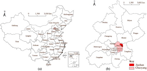
Maps showing the evacuation path network and the locations of Jinzhan’s 15 communities and 10 candidate shelters are presented in Figure 5, which was provided by the Key Laboratory of Environmental Change and Natural Disaster of Ministry of Education, Beijing Normal University. In Figure 5, in consideration of the potential damage that can be caused by an earthquake, the locations of shelters should be at least a distance of 500 m from the earthquake faults (Hu et al. 2014).

The road network is as shown in Figure 2a that has 740 paths and 521 path nodes. Based on this road network, ArcGIS mapping software (ESRI 2011) was used to determine the length of each path and subsequently, via Dijkstra’s algorithm (Dijkstra 1959), the length of the shortest evacuation route, d_kij, from sub-community i of community j to candidate shelter k within the EMS stage of the model (see Appendix I), and from EG i of EMS j to candidate shelter k within the LTS stage of the model (see Appendix II). ArcGIS mapping software was also used to determine the area of each of the 10 candidate shelters shown in Figure 2 (see Appendix I). The width of each path in the case study area was obtained using Google Earth. Further, the adjustment factor (see Equation (4)(4) $$W_{\mathit{kij}}=\sum _{q=1}^Q\left(H_{\mathit{qkij}}\times w_q\times {\alpha }_q\times \frac{l_q}{d_{\mathit{kij}}}\right)$$(4) in Section 3.1.1) associated with each path was determined in relation to the earthquake scenario considered, which is described in Section 2.2.

Figure 2. Evacuation paths, communities, shelters and distribution of population in Jinzhan.

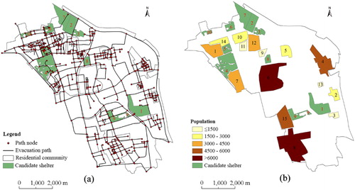
In the EMS stage of the model, the number of people within each community was divided into a set of sub-communities consisting of up to 1000 people. For example, community ‘1’ consisting of 3848 people was divided into four sub-communities; three of these with 1000 people and the other with 848. Appendix I presents a table in which the first column indicates the index of each community and the number of sub-communities within them (in brackets); the second column indicates the number of people in each of the 15 communities. The same approach as described for the model’s EMS stage was used in the LTS stage in relation to dividing the number of people in each EMS into EGs, which may consist of people from different sub-communities.

2.2. Earthquake scenario

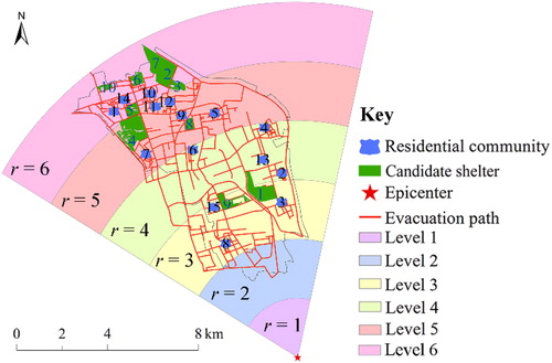
In this case study, a 6.5 magnitude earthquake with its epicentre in the Tongzhou district of Beijing is considered. In Figure 1(b), the Tongzhou district, in which an earthquake of this magnitude occurred in 1665, is south-east of the Chaoyang district. Figure 3 indicates the location of the earthquake’s epicentre in relation Jinzhan.

Figure 3. Damage level of Jinzhan.

In terms of earthquake intensity, Equation (1)(1) $$I_p=-1.82+1.32M_e-0.0106D_{e,p}$$(1) states the specific form of Equation (2)(2) $$\min f_1=\sum _{j=1}^M\sum _{i=1}^{n_{\text{sc},j}}\sum _{k=1}^N\left(\frac{d_{\mathit{kij}}}{v_{\mathit{ij}}}\times \frac{P_{\mathit{ij}}}{W_{\mathit{kij}}}\times B_{\mathit{kij}}\right)$$(2) in Appendix III for Jinzhan obtained using historical data (Zhang et al. 2009). (1) $$I_p=-1.82+1.32M_e-0.0106D_{e,p}$$(1)

With a magnitude of 6.5 at its epicentre, the earthquake’s intensity at this location is 6.760. At the farthest point (15.537 km) from the epicentre in the affected case study area, the intensity is 6.595. Correspondingly, via Equation (5)(5) $${\alpha }_q=\sum _{r=1}^{r_u}\left(\frac{l_{\mathit{qr}}}{l_q}\times \left(1-\frac{D{R}_r^i+D{R}_r^o}{2}\right)\right)$$(5) , the damage ratio varies from 0.519 at the farthest point to 0.552 at the epicentre as shown in Appendix IV. Thus, the upper index of damage level r_u, was determined as 6 using the iterative, three-step method described in Appendix III.

3. Problem formulation and mathematical model

An earthquake shelter can be defined as being either an EMS or a LTS (Beijing Municipal Institute of City Planning & Design 2007). EMSs are equipped to accommodate people for the first day after an earthquake whereas LTSs can be used to house people for up to one month or longer. To determine the number and location of EMSs and LTSs from a set of candidate shelters, as well as the allocation of evacuees to them in the first day and then beyond, a hierarchical mathematical model has been developed and is presented in this article.

An overview of the earthquake EMS and LTS location-allocation problem considered in this article is illustrated in Figure 4.

Figure 4. The EMS and LTS location-allocation problem.

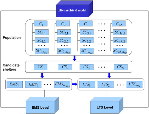
The hierarchical model, allied with an optimization algorithm, leads to the selection of n_ems EMS locations from a set of N candidate shelter (abbreviated as CS) locations; these EMSs are designated as shelters to which evacuees from all sub-communities (abbreviated as SC) of each of M communities (abbreviated as C) are allocated. Initially, while all communities have different locations, all sub-communities within a community have the same location. Also, people within the same sub-community will be allocated to the same EMS. Subsequently, the locations of n_lts LTSs are determined, some of which may have been initially selected as EMSs. Simultaneously, evacuees initially housed in EMSs are divided into groups of evacuees and allocated to LTSs. The hierarchical model is defined by the equations and constraints presented in Equations (1–12). In relation to these equations and constraints, a nomenclature is given in Appendix V.

3.1 EMS stage of the model

The two objectives related to the EMS stage of the model are to minimize: (i) total weighted evacuation time for sub-communities to travel from their respective community’s location to EMSs (TWET_EMS), f₁ (see Equation (1)(1) $$I_p=-1.82+1.32M_e-0.0106D_{e,p}$$(1) ); (ii) total shelter area of EMSs (TSA_EMS) to which sub-communities are allocated, f₂ (see Equation (5)(5) $${\alpha }_q=\sum _{r=1}^{r_u}\left(\frac{l_{\mathit{qr}}}{l_q}\times \left(1-\frac{D{R}_r^i+D{R}_r^o}{2}\right)\right)$$(5) ).

3.1.1 Total weighted evacuation time for sub-communities to travel from their respective community’s location to EMSs (TWET_EMS)

The TWET_EMS objective function is defined as (2) $$\min f_1=\sum _{j=1}^M\sum _{i=1}^{n_{\text{sc},j}}\sum _{k=1}^N\left(\frac{d_{\mathit{kij}}}{v_{\mathit{ij}}}\times \frac{P_{\mathit{ij}}}{W_{\mathit{kij}}}\times B_{\mathit{kij}}\right)$$(2) where $n_{\mathrm{sc},j}$ is the number of sub-communities in community j. In Equation (2)(2) $$\min f_1=\sum _{j=1}^M\sum _{i=1}^{n_{\text{sc},j}}\sum _{k=1}^N\left(\frac{d_{\mathit{kij}}}{v_{\mathit{ij}}}\times \frac{P_{\mathit{ij}}}{W_{\mathit{kij}}}\times B_{\mathit{kij}}\right)$$(2) , d_kij is the length of the shortest evacuation route, which is made up of one or more paths, from sub-community i of community j to candidate shelter k. In this article, as a simplification, all of the people within the same sub-community travel to the shelters to which they are allocated at an average evacuation speed, v_ij, which is calculated via Equation (3)(3) $$v_{\mathit{ij}}=(2\times p_{j\mathrm{c}}\times v_{\mathrm{c}})+\left(\right(p_{j\mathrm{a}}-p_{j\mathrm{c}})\times v_{\mathrm{a}})+(p_{j\mathrm{e}}\times v_{\mathrm{e}})$$(3) , (3) $$v_{\mathit{ij}}=(2\times p_{j\mathrm{c}}\times v_{\mathrm{c}})+\left(\right(p_{j\mathrm{a}}-p_{j\mathrm{c}})\times v_{\mathrm{a}})+(p_{j\mathrm{e}}\times v_{\mathrm{e}})$$(3) where p_jc, p_ja and p_je are the proportions of community j’s children, adults and elderly people, respectively, and v_c, v_a and v_e represent the speed of children, adults and elderly people in all communities. In Equation (3)(3) $$v_{\mathit{ij}}=(2\times p_{j\mathrm{c}}\times v_{\mathrm{c}})+\left(\right(p_{j\mathrm{a}}-p_{j\mathrm{c}})\times v_{\mathrm{a}})+(p_{j\mathrm{e}}\times v_{\mathrm{e}})$$(3) , it is noted that an adult will help a child and thus the speed of this adult is same as that of the child. In the case study presented in this article, the speed of children, v_c, adults, v_a and elderly people, v_e, is 1.05, 1.27 and 1.12 m/s, respectively (Gates et al. 2006). Further, the proportions of children, adults and elderly people in each of Jinzhan’s 15 communities was determined using population data provided by the Beijing Bureau of Civil Affairs. Due to the limited data available, these proportions were taken to be constant for all communities, i.e. p_jc = 0.025, p_ja = 0.928 and p_je = 0.047.

In Equation (2)(2) $$\min f_1=\sum _{j=1}^M\sum _{i=1}^{n_{\text{sc},j}}\sum _{k=1}^N\left(\frac{d_{\mathit{kij}}}{v_{\mathit{ij}}}\times \frac{P_{\mathit{ij}}}{W_{\mathit{kij}}}\times B_{\mathit{kij}}\right)$$(2) , the quotient involving P_ij and W_kij is included to adjust the evacuation time due to the congestion of evacuation paths. The parameter P_ij represents the number of people within sub-community i of community j. The parameter W_kij is the weighted mean width of the evacuation paths that form the entire route taken by sub-community i of community j to candidate shelter k; the term weighted is used to indicate that the length, as well as width, of each path that forms the evacuation route is considered in determining W_kij as shown in Equation (4)(4) $$W_{\mathit{kij}}=\sum _{q=1}^Q\left(H_{\mathit{qkij}}\times w_q\times {\alpha }_q\times \frac{l_q}{d_{\mathit{kij}}}\right)$$(4) . (4) $$W_{\mathit{kij}}=\sum _{q=1}^Q\left(H_{\mathit{qkij}}\times w_q\times {\alpha }_q\times \frac{l_q}{d_{\mathit{kij}}}\right)$$(4)

In Equation (4)(4) $$W_{\mathit{kij}}=\sum _{q=1}^Q\left(H_{\mathit{qkij}}\times w_q\times {\alpha }_q\times \frac{l_q}{d_{\mathit{kij}}}\right)$$(4) , the parameter Q is the total number of paths in an earthquake affected case study area and the variable H_qkij indicates whether or not path q forms part of the evacuation route taken by sub-community i of community j to shelter k, i.e. H_qkij = 1 if path q forms part of the evacuation route whereas H_qkij = 0 if not. Furthermore, w_q represents the width of path q which forms part of the evacuation route. To account for earthquake damage to each path making up an evacuation route, the parameter w_q is modified using an adjustment factor, α_q, which is calculated using Equation (5)(5) $${\alpha }_q=\sum _{r=1}^{r_u}\left(\frac{l_{\mathit{qr}}}{l_q}\times \left(1-\frac{D{R}_r^i+D{R}_r^o}{2}\right)\right)$$(5) , (5) $${\alpha }_q=\sum _{r=1}^{r_u}\left(\frac{l_{\mathit{qr}}}{l_q}\times \left(1-\frac{D{R}_r^i+D{R}_r^o}{2}\right)\right)$$(5) where r is the damage level index associated with an earthquake affected case study area ranging from 1 to an upper value, termed r_u; lower values of r signify areas closer to the earthquake’s epicentre as shown in Figure 5.

Figure 5. Damage level areas and indices of an earthquake affected case study area.

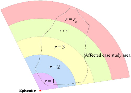
The upper damage level index, r_u, is determined via an iterative, three-step method as shown in Appendix III. The index l_qr and l_q represent the length of the path in the damage level area and total path length. The index ${\mathit{DR}}_r^i$ and ${\mathit{DR}}_r^o$ are inner boundary and outer boundary of damage level area r.

Returning to Equation (2)(2) $$\min f_1=\sum _{j=1}^M\sum _{i=1}^{n_{\text{sc},j}}\sum _{k=1}^N\left(\frac{d_{\mathit{kij}}}{v_{\mathit{ij}}}\times \frac{P_{\mathit{ij}}}{W_{\mathit{kij}}}\times B_{\mathit{kij}}\right)$$(2) , the variable B_kij indicates whether or not sub-community i of community j is allocated to candidate shelter k (providing it has been selected as a shelter), i.e. B_kij = 1 if allocated whereas B_kij = 0 if not.

3.1.2 Total shelter area of EMSs (TSA_EMS) to which sub-communities are allocated

The TSA_EMS objective function is defined as (6) $$\min f_2=\sum _{k=1}^N\left(X_k\times S_k\right)$$(6) where X_k indicates whether or not candidate shelter k is selected as an EMS, i.e. X_k = 1 if selected, otherwise X_k = 0. Further, the parameter S_k indicates the available area of candidate shelter k. In the case study described in Section 3, S_k is defined as 60% of a shelter’s area due to only this proportion being able to be used to house evacuees whereas the remaining 40% is unsuitable (Beijing Municipal Institute of City Planning & Design 2007).

3.1.3 Constraints of EMSs

The constraints associated with the model’s EMS stage are related to evacuation time (see Constraint (7)(7) $$d_{\mathit{kij}}\times B_{\mathit{kij}}-D_{\mathit{ij}}\le 0,\forall i=1,2,\dots ,n_{\text{sc},j}; \forall j=1,2,\dots ,n_{\text{ems}};\forall k=1,2,\dots ,N$$(7) ), shelter capacity (see Constraint (8)(8) $$\sum _{j=1}^M\sum _{i=1}^{n_{\text{sc},j}}\left(P_{\mathit{ij}}\times B_{\mathit{kij}}-C_k\times X_k\right)\le 0,\forall k=1,2,\dots ,N$$(8) ), and ensuring that a sub-community of a community can be allocated to only one shelter (see Constraint (9)(9) $$\sum _{k=1}^N\left(B_{\mathit{kij}}\times X_k\right)=1,\forall i=1,2,\dots ,n_{\text{sc},j}; \forall j=1,2,\dots ,n_{\text{ems}}$$(9) ). (7) $$d_{\mathit{kij}}\times B_{\mathit{kij}}-D_{\mathit{ij}}\le 0,\forall i=1,2,\dots ,n_{\text{sc},j}; \forall j=1,2,\dots ,n_{\text{ems}};\forall k=1,2,\dots ,N$$(7) (8) $$\sum _{j=1}^M\sum _{i=1}^{n_{\text{sc},j}}\left(P_{\mathit{ij}}\times B_{\mathit{kij}}-C_k\times X_k\right)\le 0,\forall k=1,2,\dots ,N$$(8) (9) $$\sum _{k=1}^N\left(B_{\mathit{kij}}\times X_k\right)=1,\forall i=1,2,\dots ,n_{\text{sc},j}; \forall j=1,2,\dots ,n_{\text{ems}}$$(9)

In Constraint (7)(7) $$d_{\mathit{kij}}\times B_{\mathit{kij}}-D_{\mathit{ij}}\le 0,\forall i=1,2,\dots ,n_{\text{sc},j}; \forall j=1,2,\dots ,n_{\text{ems}};\forall k=1,2,\dots ,N$$(7) , the parameter D_ij is the maximum evacuation distance that sub-community i of community j can travel in t_ij seconds if moving at speed v_ij as defined in Equation (3)(3) $$v_{\mathit{ij}}=(2\times p_{j\mathrm{c}}\times v_{\mathrm{c}})+\left(\right(p_{j\mathrm{a}}-p_{j\mathrm{c}})\times v_{\mathrm{a}})+(p_{j\mathrm{e}}\times v_{\mathrm{e}})$$(3) . The parameter t_ij is set to 4600 s in order to ensure that each sub-community in the case study area can reach at least two candidate shelters. In Constraint (8)(8) $$\sum _{j=1}^M\sum _{i=1}^{n_{\text{sc},j}}\left(P_{\mathit{ij}}\times B_{\mathit{kij}}-C_k\times X_k\right)\le 0,\forall k=1,2,\dots ,N$$(8) , the parameter C_k is the accommodation capacity of candidate shelter k as an EMS, i.e. the number of evacuees that can be housed in shelter k. This parameter can be determined by dividing S_k (see Equation (6)(6) $$\min f_2=\sum _{k=1}^N\left(X_k\times S_k\right)$$(6) ) by the average area occupied by a single person. For an EMS, given that evacuees will stay for only a short period of time, a small area, 1 m², is needed per person (Beijing Municipal Institute of City Planning & Design 2007).

3.2 LTS stage of the model

The results of the EMS stage of the model provide the input for the LTS stage, which is then solved to determine the location of LTSs and how the evacuees are allocated to them from EMSs. The model’s LTS stage includes two objectives which are to minimize: (i) total weighted evacuation time for groups of evacuees, potentially consisting of people from different sub-communities, to travel from EMSs to LTSs (TWET_LTS), f₃ (see Equation (10)(10) $$\min f_3=\sum _{j=1}^{n_{\text{ems}}}\sum _{i=1}^{n_{\text{eg},j}}\sum _{k=1}^N\left(\frac{d_{\mathit{kij}}}{v_{\mathit{ij}}}\times \frac{P_{\mathit{ij}}}{W_{\mathit{kij}}}\times B_{\mathit{kij}}\right)$$(10) ); (ii) total shelter area of LTSs (TSA_LTS) to which groups of evacuees are allocated, f₄ (see Equation (11)(11) $$\min f_4=\sum _{k=1}^N\left(X_k\times S_k\right)$$(11) ).

3.2.1 Total weighted evacuation time for groups of evacuees to travel from EMSs to LTSs (TWET_LTS)

The TWET_LTS objective function is defined as (10) $$\min f_3=\sum _{j=1}^{n_{\text{ems}}}\sum _{i=1}^{n_{\text{eg},j}}\sum _{k=1}^N\left(\frac{d_{\mathit{kij}}}{v_{\mathit{ij}}}\times \frac{P_{\mathit{ij}}}{W_{\mathit{kij}}}\times B_{\mathit{kij}}\right)$$(10)

Equation (10)(10) $$\min f_3=\sum _{j=1}^{n_{\text{ems}}}\sum _{i=1}^{n_{\text{eg},j}}\sum _{k=1}^N\left(\frac{d_{\mathit{kij}}}{v_{\mathit{ij}}}\times \frac{P_{\mathit{ij}}}{W_{\mathit{kij}}}\times B_{\mathit{kij}}\right)$$(10) is similar to Equation (2)(2) $$\min f_1=\sum _{j=1}^M\sum _{i=1}^{n_{\text{sc},j}}\sum _{k=1}^N\left(\frac{d_{\mathit{kij}}}{v_{\mathit{ij}}}\times \frac{P_{\mathit{ij}}}{W_{\mathit{kij}}}\times B_{\mathit{kij}}\right)$$(2) ; however the summation limits differ in that: (a) i varies from 1 to the number of groups of evacuees situated in EMS j, n_eg,j, each of which may consist of people from the same or different sub-communities (as opposed to the number of sub-communities of community j, n_sc,j, as seen in Equation (2)(2) $$\min f_1=\sum _{j=1}^M\sum _{i=1}^{n_{\text{sc},j}}\sum _{k=1}^N\left(\frac{d_{\mathit{kij}}}{v_{\mathit{ij}}}\times \frac{P_{\mathit{ij}}}{W_{\mathit{kij}}}\times B_{\mathit{kij}}\right)$$(2) ); (b) j varies from 1 to the number of EMSs, n_ems, (rather than the number of communities, M, as seen in Equation (2)(2) $$\min f_1=\sum _{j=1}^M\sum _{i=1}^{n_{\text{sc},j}}\sum _{k=1}^N\left(\frac{d_{\mathit{kij}}}{v_{\mathit{ij}}}\times \frac{P_{\mathit{ij}}}{W_{\mathit{kij}}}\times B_{\mathit{kij}}\right)$$(2) ).

3.2.2 Total shelter area of LTSs (TSA_LTS) to which groups of evacuees are allocated

The TSA_LTS objective function is defined as (11) $$\min f_4=\sum _{k=1}^N\left(X_k\times S_k\right)$$(11) Equation (11)(11) $$\min f_4=\sum _{k=1}^N\left(X_k\times S_k\right)$$(11) is similar to Equation (6)(6) $$\min f_2=\sum _{k=1}^N\left(X_k\times S_k\right)$$(6) ; however the variable X_k indicates whether or not candidate shelter k is selected as an LTS (rather than selected as an EMS as in Equation (6)(6) $$\min f_2=\sum _{k=1}^N\left(X_k\times S_k\right)$$(6) ).

3.2.3 Constraints of LTSs

The constraints associated with the model’s EMS stage are related to the shelter capacity constraint (see Constraint (12)), and ensuring that an EG from an EMS can be allocated to only one LTS (see Constraint (13)). (12) $$\sum _{j=1}^{n_{\text{ems}}}\sum _{i=1}^{n_{\text{eg},j}}\left(P_{\mathit{ij}}\times B_{\mathit{kij}}-C_k\times X_k\right)\le 0,\forall k=1,2,\dots ,N$$(12) (13) $$\sum _{k=1}^N\left(B_{\mathit{kij}}\times X_k\right)=1,\forall i=1,2,\dots ,n_{\text{eg},j}; \forall j=1,2,\dots ,n_{\text{ems}}$$(13)

Constraint (12) is similar to Constraint (8)(8) $$\sum _{j=1}^M\sum _{i=1}^{n_{\text{sc},j}}\left(P_{\mathit{ij}}\times B_{\mathit{kij}}-C_k\times X_k\right)\le 0,\forall k=1,2,\dots ,N$$(8) ; however, the summation limits differ as stated in Section 2.2.1, and C_k is the accommodation capacity of candidate shelter k as an LTS (rather than the capacity of the shelter as an EMS as in Constraint (8)(8) $$\sum _{j=1}^M\sum _{i=1}^{n_{\text{sc},j}}\left(P_{\mathit{ij}}\times B_{\mathit{kij}}-C_k\times X_k\right)\le 0,\forall k=1,2,\dots ,N$$(8) ). The parameter C_k can be determined by dividing S_k (see Equation (11)(11) $$\min f_4=\sum _{k=1}^N\left(X_k\times S_k\right)$$(11) ) by the average area occupied by a single person in an LTS, which is defined as 3 m² (Beijing Municipal Institute of City Planning & Design 2007).

4. Interleaved MPSO–GA

In this research, due to the multi-objective nature of each stage of the mathematical model, coupled with these objectives being conflicting, an interleaved MPSO–GA combining a GA and MPSO algorithm has been implemented to solve the model. A nomenclature related to these algorithms is given in Appendix VI.

The interleaved MPSO–GA (see Figure 6(a)) begins with an initial population of size 200 being randomly generated, via the INITIALIZE function, followed by the MPSO algorithm (see Figure 6(b)) being executed to solve the location-allocation problem. In each iteration, the solution is compared with the solution generated in the previous iteration, and the non-dominated solution PS is updated with the function NONDOMINATED. After the first one hundred iterations of the MPSO algorithm, and each subsequent iteration, the current Pareto set is assessed against the previous fifty Pareto sets such that if no difference exists between them, i.e. convergence it taken as having occurred, then the execution passes from the MPSO algorithm to the GA (see Figure 6(c)). The GA continues to be executed until no difference exists between the Pareto sets in the same way as described for the MPSO algorithm. Also, at this point, execution passes from the GA to the MPSO algorithm. This process of interleaving the execution of the MPSO algorithm and GA continues until the convergence of the Pareto sets is met simultaneously by both algorithms. It is noted that when changing from one algorithm to the other, the population generated in the last iteration is taken as the initial population of the algorithm to be executed. The decision to compare the current Pareto set with the previous fifty Pareto sets in order to establish if convergence had occurred was determined via experimentation.

Figure 6. Interleaved MPSO–GA.

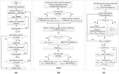
Figure 6(b) presents the MPSO algorithm (Zhao et al. 2015). With a population size of 200, each iteration, the movement of any particle, u, through the search space is informed by its knowledge of the best position it has occupied so far in terms of objective value(s), p_best,u, and the position of the particle with the best objective value(s) so far within (a) neighbouring particles, n_best,u, (von Neumann topology) or (b) all particles, g_best, (global topology).

For each iteration of the MPSO algorithm, the TWET and TSA objective values associated with each particle are evaluated using the COMPUTEOV function that uses Equations (1)(1) $$I_p=-1.82+1.32M_e-0.0106D_{e,p}$$(1) and (5)(5) $${\alpha }_q=\sum _{r=1}^{r_u}\left(\frac{l_{\mathit{qr}}}{l_q}\times \left(1-\frac{D{R}_r^i+D{R}_r^o}{2}\right)\right)$$(5) for the EMS stage and Equations (9)(9) $$\sum _{k=1}^N\left(B_{\mathit{kij}}\times X_k\right)=1,\forall i=1,2,\dots ,n_{\text{sc},j}; \forall j=1,2,\dots ,n_{\text{ems}}$$(9) and (10)(10) $$\min f_3=\sum _{j=1}^{n_{\text{ems}}}\sum _{i=1}^{n_{\text{eg},j}}\sum _{k=1}^N\left(\frac{d_{\mathit{kij}}}{v_{\mathit{ij}}}\times \frac{P_{\mathit{ij}}}{W_{\mathit{kij}}}\times B_{\mathit{kij}}\right)$$(10) for the LTS stage. Next, the velocity and position of each particle are updated using the functions UPDATE_v and UPDATE_p. For velocity updating, in this research, based on experimentation, to achieve a balance between exploration and exploitation, the von Neumann topology is used in the MPSO algorithm’s first one hundred iterations and thereafter the global topology is used. Subsequently, for each particle, if its current position, p_current, is better than its best position so far, p_best, then p_current becomes p_best. However, if p_current is worse than p_best, then in contrast to a general PSO algorithm, SA is applied to update p_best such that a worse position has the potential of being accepted, albeit with a lower probability than a better position. Following the update of p_best, Algorithm 2 determines the position of the particle with the best objective value(s) so far within (a) neighbouring particles, n_best, (von Neumann topology) or (b) all particles, g_best, (global topology). Here, p_nns is updated via the UPDATE_n function, which compares the positions of neighbours of a particle, p_n, and the positons of particles in the non-dominated set obtained by neighbours so far. Similarly, p_gs is updated with via the UPDATE_g function, which compares the positions of all particles, p_g, and the positons of particles in the Pareto set.

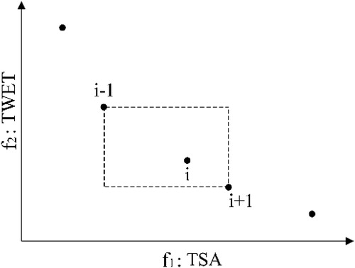
In relation to n_best and g_best, the particle selected, via the SELECT function, is that with the largest rectangular area unoccupied by any other solutions as shown in Figure 7’s visual representation of the search space. Selecting n_best and g_best in this manner facilitates a search within its local proximity that may lead to a better solution being found. This selection approach is adapted from the use of crowding distance by Deb et al. (2002).

Figure 7. Particle selection.

Figure 6(c) presents the GA implemented in this research, which was developed via experimentation. In the GA, with the initial population of size 200 being taken from the last iteration of the MPSO algorithm, each iteration of the GA uses a COMPUTEFITNESS function to evaluate the fitness of each individual in the current population. The fitness of individual u, f_u, is calculated using Equation (20)(20) $$f_u=n+1-R_u$$(20) , (20) $$f_u=n+1-R_u$$(20) where n is the number of individuals in the population and R_u is the rank of individual u based on dominance in relation to the TWET and TSA objectives (for both the model’s EMS and LTS stages).

In the GA, once each individual’s fitness has been evaluated, the fittest 5% of individuals in the current generation, i.e. iteration of the GA, are preserved as P_elite using the ELITE function; later in the GA these replace the worst 5% of individuals in the next generation. The procedure of determining the next generation involves using selection, crossover and mutation operations. The selection of individuals from the population, via the SELECTION_p function, involves the use of a fitness sharing method and a roulette wheel based approach (Goldberg 1989). Next, depending on the crossover probability, c, the selected individual can either (a) mate with another individual, via the CROSSOVER function, to produce offspring to be included in the next generation, or (b) be copied directly to the next generation. In the GA developed in this research, experimentation has established that a good value of c is 0.95. In the SELECTION_p_mate function, a strategy is applied such that only a sufficiently different individual within a specified proximity in the search space can be selected as a mate for another individual. Again, via experimentation, it was determined that an individual can only be selected as the mate of another individual providing their respective chromosomes are at least 30% different and they are a Euclidean distance of <5,000,000 apart in the TWET-TSA search space. In relation to the CROSSOVER function, a method proposed by Haupt and Haupt (1998) is used in which uniform point crossover is combined with a blend of the genes of two parents to produce two offspring. Once the next generation is fully populated, each individual can be mutated, via the MUTATE function, according to the mutation probability, m, which in this implementation of a GA is set to 0.04 based on an experimental analysis. Furthermore, the fittest 1% of individuals is immune from mutation. As referred to earlier, within the next generation, P_next, the worst 5% of individuals, P_worst, selected via the WORST function are replaced by the fittest 5% of individuals preserved from the last generation, P_elite.

5. Results and discussion

Initially, this section presents a comparison of the algorithms mentioned in Section 4 demonstrating that the interleaved MPSO–GA yields better solutions to the earthquake shelter location-allocation problem than if the MPSO algorithm or GA were used in isolation. Following this comparison, in the context of the case study area of Jinzhan within the Chaoyang district of Beijing in China, results are presented from the application of the interleaved MPSO–GA to the model’s EMS and LTS stage, respectively.

5.1 Comparison of the MPSO algorithm, GA and interleaved MPSO–GA

In order to compare the algorithms discussed in Section 4, the EMS stage of the mathematical model was used in which the location of the EMSs is to be determined along with the allocation of sub-communities to them. Fifteen replicates were performed using each algorithm; however, it was observed that no additional Pareto solutions were found beyond seven executions of the MPSO algorithm and GA, and beyond two executions of the interleaved MPSO–GA. For the MPSO algorithm and GA, 2500 iterations were performed each execution as this was found, via experimentation, to give convergence. However, in using the interleaved MPSO–GA, an average of only 1135 iterations was required before convergence of the Pareto sets of the MPSO algorithm and GA was met simultaneously. Figure 8 shows the Pareto solutions obtained using each algorithm.

Figure 8. Pareto optimal solutions obtained by different algorithms.

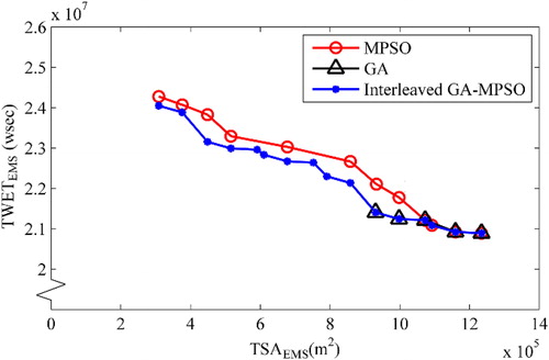
In Figure 8, it can be seen that predominantly the interleaved MPSO–GA outperforms both the MPSO algorithm and GA in terms of generating Pareto optimal solutions that minimize the TWET_EMS and TSA_EMS objectives. It is noted that the units of the TWET_EMS objective is weighted seconds, which not only accounts for the distance travelled along the shortest evacuation route at a particular speed, but also considers the damage to these routes and the number of people moving along them. The Pareto optimal set obtained by the GA is smaller than that obtained by the other two algorithms. In contrast, the Pareto optimal set obtained using the MPSO algorithm spans the same solution space, in terms of TWET_EMS and TSA_EMS, as the interleaved MPSO–GA; although the number of Pareto solutions is less (12 compared against 16) and these are dominated by those obtained using the interleaved MPSO–GA.

Based on the findings of the comparison presented, the interleaved MPSO–GA was used to solve the hierarchical mathematical model of the earthquake shelter location-allocation problem.

5.2 Results of the earthquake shelter location-allocation model

This section presents the results obtained by the interleaved MPSO–GA in solving the mathematical model’s EMS stage and then the LTS stage. Figure 9 shows the Pareto optimal set obtained which consists of 16 solutions.

Figure 9. Pareto optimal set of EMS stage.

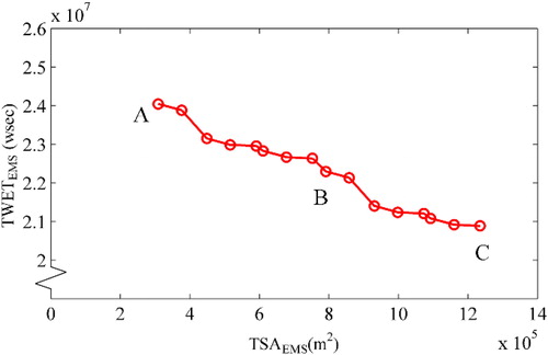
Figure 9 indicates that if sub-communities are to be evacuated in less time than more EMSs, or larger EMSs nearer to sub-communities, need to be constructed. Taking solutions on the Pareto front marked ‘A’, ‘B’ and ‘C’ in Figure 9 as examples, the location of selected candidate shelters to be used as EMSs and how the sub-communities are allocated to them are shown in Figure 10(a–c), respectively. In Figure 10, it can be seen that all sub-communities belonging to the same community are allocated to the same EMSs. For example, in Figure 10(a), all sub-communities from 10 communities are allocated to candidate shelter 8 whereas those from five communities are allocated to candidate shelter 9. As indicated in Figure 10(b,c), three (1, 8, 9) and five (1, 2, 6, 8, 9) candidate shelters are used as EMSs.

Figure 10. EMS stage result corresponding to Pareto solution (a) A, (b) B and (c) C.

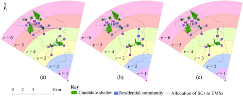
In Figure 11, it can be seen that for Pareto solutions ‘A’, ‘B’ and ‘C’, shelters 8 and 9 are always selected as EMSs. Further, all sub-communities from communities 1, 5, 6, 7, 9 and 11 are always allocated to shelter 8 whereas all sub-communities from communities 8 and 15 are always allocated to shelter 9. As shown in Figure 9, the TWET_EMS objective decreases from Pareto optimal solution ‘A’ to ‘B’. The difference between these two solutions, as illustrated in Figure 10(a,b), is that solution ‘B’ also includes shelter 1 as an EMS. Further, all sub-communities from communities 2, 3 and 13 are allocated to this shelter, rather than shelter 9 as for solution ‘A’, since it is nearer to them. Similarly, sub-communities from community 4 are allocated to shelter 1 rather than shelter 8. In consideration of the Pareto optimal solution labelled ‘C’ in Figure 9, shelters 2 and 6 are added to 1, 8 and 9 as EMSs as shown in Figure 10(c). Also, all sub-communities from communities 10, 12 and 14 are allocated to shelters 2 and 6.

Figure 11. Pareto optimal set of LTSs.

The solution to the EMS stage of the model forms the input for the LTS stage. Thus, each of the sixteen Pareto solutions for the model’s EMS stage shown in Figure 9 will lead to a different Pareto optimal set of solutions to the LTS stage. In this research, the Pareto solution with the lowest TWET_EMS for the EMS stage, labelled ‘C’ in Figure 9 and illustrated in Figure 10(c), was selected as the input for the LTS stage. In this solution, sub-communities from communities are allocated to EMSs as indicated in Table 1. Within the LTS stage of the model, the sub-communities allocated to the five EMS are divided into 61 EGs in each of which the number of people is up to 1000. The number of EGs in each EMS to be allocated to LTSs is shown in Table 1.

Table 1. EMS location-allocation and the EG of each EMS.

EMS ID	1				2		6	8						9
Community ID	2	3	4	13	10	12	14	1	5	6	7	9	11	8	15
No. of people	8935				6168		2084	23,337						17,476
No. of EGs	9				7		3	24						18

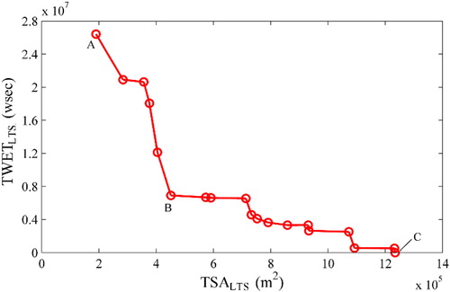
In the LTS stage of the model, all 10 original candidate shelters can potentially become LTSs, five of which were selected as EMSs after solving the model’s EMS stage. Thus, on solving the LTS stage of the model, an EMS may become an LTS. On applying the interleaved MPSO–GA to solve the LTS stage of the model, the Pareto optimal set containing 19 solutions was obtained as shown in Figure 10.

In Figure 11, the solutions labelled ‘A’ and ‘C’ signify those at either end of the Pareto front, and the solution labelled ‘B’ is located approximately at the mid-point. In comparing solutions ‘A’ and ‘B’, both with a TSA_LTS <500,000 m², TWET_LTS decreases sharply from 26.4 to 6.9 million weighted seconds. However, in comparing solutions ‘B’ and ‘C’, as TSA_LTS increase from 500,000 m² to approximately 1,200,000 m², TWET_LTS decreases gradually from 6.9 million weighted seconds to zero. A TWET_LTS of zero corresponds with a solution to the LTS stage of the model that is the same as that obtained at the EMS stage; thus EGs are not reallocated from EMSs to LTSs.

For the solutions on the Pareto front in Figure 11 marked ‘A’, ‘B’ and ‘C’, Figure 12(a–c) shows the candidate shelters to be used as LTSs and includes lines indicating which EGs are allocated to them.

Figure 12. EMS and LTS location-allocation of Pareto solution A, B and C.

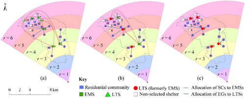
In Figure 12, it can be seen that all EGs located in an EMS can be allocated to different LTSs or the same LTS. For example, in Figure 12(a), EGs from EMS 1 are allocated to LTS 3 and 10 whereas all EGs from EMS 2 are allocated to LTS 10. As indicated in Figures 12(b), shelters 6, 8, 9 initially selected as EMSs go on to be selected as LTSs. Also, as shown in Figure 12(c), all shelters initially selected as EMSs go on to be selected as LTSs. Thus, evacuees allocated to shelters in solving the EMS stage of the model are not reallocated in the LTS stage. In contrast, in Figure 12(b), all EGs allocated to EMS 2 are reallocated to LTS 6. Similarly, some EGs in EMS 1 are reallocated to LTSs 6 and 8.

Table 2 presents details of the three Pareto solutions discussed. In addition to indicating the index of shelters selected as EMSs and LTSs, Table 2 specifies how many evacuees are allocated to the LTSs and the time taken for them to evacuate from their designated EMS to LTS. It is noted that the evacuation times stated represent the actual time for EGs to travel from their respective EMS to their designated LTS, taking into account the number of evacuees and the earthquake damage to evacuation routes. In Pareto solution A, only two LTSs are selected, namely 3 and 10, to which all evacuees in EMSs are reallocated. All evacuees in EMS 2 and 6 are reallocated to LTS 10, and most evacuees in other EMSs are allocated to LTS 10 but some to LTS 3. There are two advantages of Pareto solution A compared with solutions B and C: (i) the value of TSA is less than that of Pareto solutions B and C, which represents the total cost for LTS is less assuming the constructing cost of shelters is same per square metre; (ii) the two LTSs, i.e. 3 and 10, are located far from the epicentre of the earthquake, which means LTSs of solution A is safer than LTSs of solutions B and C. However, it has a disadvantage in that all of evacuees in EMSs should be reallocated and thus the total evacuation time is longer than for Pareto solutions B and C. For Pareto solution B, only evacuees in EMS 1 and 2 need to be reallocated to LTS 6 and 8. The advantages of this solution are that it provides a balance between evacuation time and shelter area. Further, the evacuation time is less than that for Pareto solution A; however, it is more than for Pareto solution C. In Pareto solution C, all EMSs are assigned as LTSs meaning that all evacuees can remain in their initial shelters. Thus, the advantage of this solution is that the evacuees do not need to reallocated. However, this solution’s disadvantages are that the value of TSA, representing of total cost of LTSs construction, is more than that of Pareto solutions A and B and there are two LTSs near to the earthquake’s epicentre, i.e. shelter 1 and 9, which will accommodate 26,411 people.

Table 2. EMS and corresponding LTS and evacuation time of Pareto solution A, B and C.

PS A	EMS ID	1		2	6	8		9
	LTS ID	3	10	10	10	3	10	3	10
	No. of people	7935	1000	6168	2084	17,337	6000	14,476	3000
	Evacuation time (s)	6994	9556	3511	1779	3073	4395	6988	7847
PS B	EMS ID	1		2	6	8		9
	LTS ID	6	8	6	6	8		9
	No. of people	2000	6935	6168	2084	23,337		17,476
	Evacuation time (s)	9031	6155	3084	0	0		0
PS C	EMS ID	1		2	6	8		9
	LTS ID	1		2	6	8		9
	No. of people	8935		6168	2084	23,337		17,476
	Evacuation time (s)	0		0	0	0		0

6. Conclusions

This article presents a new multi-objective, hierarchical mathematical model of the earthquake shelter location-allocation problem. Importantly, the model accounts for damage caused by an earthquake to evacuation routes and the effect of this on the time taken to evacuate from communities to EMSs and, subsequently, from EMSs to LTSs. Furthermore, an interleaved MPSO–GA has been used to solve the model for a particular case study in order to determine the location of EMSs and LTSs along with how evacuees should be allocated to them in the aftermath of an earthquake. In relation to the interleaved MPSO–GA developed, this has been demonstrated to yield better solutions to the earthquake shelter location-allocation problem than using either the MPSO or GA in isolation.

The model and interleaved MPSO–GA have been applied to an earthquake scenario in the case study area of Jinzhan within the Chaoyang district of Beijing in China. For this case study, in solving the model’s EMS stage, a set of sixteen Pareto solutions was obtained. Following this, taking the Pareto solution with the lowest TWET_EMS as input, the LTS stage of the model was solved yielding a set of nineteen Pareto solutions. These solutions present government with a range of options, each of which offers variations in terms of values for the TWET_LTS and TAS_LTS objectives. Thus, based on government preferences, choices can be made regarding the locations in which to construct earthquake shelters. In this article, although the model is tested with a relatively small scale problem, namely Jinzhan, in order to demonstrate the model and methods used, the model is also suitable for larger scale problems.

Future work could consider the effect of earthquake damage in more detail such as the damage caused to buildings and the effect of this in terms of obstructing evacuation routes. Another aspect of future work could focus on the time of day at which an earthquake occurs given that the distribution of the population in a given geographical area will vary as will the density of traffic. Furthermore, the adherence of evacuees in using evacuation route determined by the authorities should be taken account.

Acknowledgements

The authors gratefully acknowledge the support provided by the China Scholarship Council.

Disclosure statement

No potential conflict of interest was reported by the authors.

Additional information

Funding

The authors are thankful for the funding provided by the National Key Research and Development Program of China (No. 2018YFA1508802), the Program of Introducing Talent to Universities (No. B08008) and the National Natural Science Foundation of China (No. 41201547).

Appendix I

 

Table

			Candidate shelter index
			1	2	3	4	5	6	7	8	9	10
		Area (m^2) Population	803,385	502,342	203,617	1,114,636	232,884	236,840	741,967	157,105	357,538	112,152
Community index	1 (4)	3848	10,575.4	2920.6	4410.4	3397.1	1565.1	2351.1	3687.6	3691.3	8080.5	1981.5
	2 (2)	1650	1411.0	8488.5	7679.4	9096.8	9489.1	10,647.4	11,320.5	6626.0	4438.1	11,370.7
	3 (1)	956	1392.9	9112.8	8303.7	8965.4	9885.3	11,075.8	11,944.8	7250.3	2703.3	11,799.1
	4 (6)	5874	3492.6	7451.5	6642.4	8149.5	8452.1	9610.4	10,283.4	5589.0	5841.1	10,333.7
	5 (3)	2157	5600.8	3583.2	2774.1	4455.3	4583.8	5742.1	6415.2	1540.3	5142.3	6465.4
	6 (11)	10,937	6170.0	5173.8	5733.4	4966.2	5886.1	7076.7	8004.3	3676.7	3147.5	7800.0
	7 (5)	4251	8158.2	3875.9	4672.0	1576.7	2821.8	4012.3	5271.3	2565.4	5135.7	4735.6
	8 (13)	12,858	5375.1	8509.0	8690.2	8082.5	9002.4	10,193.0	11,339.5	7011.9	2575.6	10,916.3
	9 (9)	868	7501.7	1771.6	2125.1	3275.6	2772.2	3930.5	4603.5	360.6	5389.5	4653.8
	10 (3)	2716	9820.4	1167.3	3151.2	3341.2	2074.2	1989.5	2270.7	2936.2	7491.3	2773.2
	11 (2)	1276	8902.9	1329.4	2814.2	2856.1	1589.1	2539.8	3053.7	2018.7	6573.8	3264.3
	12 (4)	3452	8376.2	627.4	1929.2	3598.1	2664.4	3168.2	3459.3	1492.1	6169.6	3945.5
	13 (1)	455	1949.2	7778.8	6969.6	8476.7	8779.4	9937.7	10,610.7	5916.2	4976.3	10,661.0
	14 (3)	2084	10,581.3	2235.9	4246.3	3435.2	1753.1	1552.8	2918.4	3697.2	8118.6	2104.7
	15 (5)	4618	4801.5	6798.6	6851.1	6540.3	7460.2	8650.8	9629.1	5231.5	736.5	9374.1

Appendix II

 

Table

Index of Candidate shelter as LTS
Index of Candidate shelter as EMS		1	2	3	4	5	6	7	8	9	10
	1	0.0	9003.6	8194.5	9611.9	10,004.2	11,162.5	11,835.6	7141.1	4096.2	11,885.8
	2	9003.6	0.0	2232.7	4163.7	2896.7	2563.3	2831.9	2119.5	6797.0	3357.0
	3	8194.5	2232.7	0.0	5021.6	4381.6	4773.5	5064.6	2106.7	6648.4	5550.7
	4	9611.9	4163.7	5021.6	0.0	2825.9	4016.4	5275.4	2915.0	6589.4	4739.7
	5	10,004.2	2896.7	4381.6	2825.9	0.0	2749.5	4008.5	3120.1	7509.3	3472.8
	6	11,162.5	2563.3	4773.5	4016.4	2749.5	0.0	3245.9	4278.4	8699.8	1806.8
	7	11,835.6	2831.9	5064.6	5275.4	4008.5	3245.9	0.0	4951.4	9627.4	4039.6
	8	7141.1	2119.5	2106.7	2915.0	3120.1	4278.4	4951.4	0.0	5028.8	5001.7
	9	4096.2	6797.0	6648.4	6589.4	7509.3	8699.8	9627.4	5028.8	0.0	9423.1
	10	11,885.8	3357.0	5550.7	4739.7	3472.8	1806.8	4039.6	5001.7	9423.1	0.0

Appendix III

This method starts with a value of r_u = 2 which is incremented, if necessary, until a convergence condition is met related to the adjustment factor, α_q, for all paths of all evacuation routes to shelters taken by all sub-communities.

Step 1: For a particular value of r_u (again, starting at r_u=2), a radial line from the epicentre to the farthest point of the earthquake affected case study area is divided equally into r_u damage level areas (see Figure 3).

Step 2: The damage ratio, DR, which is related to earthquake intensity, I, and thus varies with location in the affected case study area, is calculated on the inner boundary, ${\mathit{DR}}_r^i,$ and outer boundary, ${\mathit{DR}}_r^o,$ of each damage level area. The damage ratio at any location, p, can be determined via Equation (1(1) $$I_p=-1.82+1.32M_e-0.0106D_{e,p}$$(1) ), (1) $$\mathit{DR}=\frac{D{R}_u-D{R}_l}{I_u-I_l}\times \left(I_p-I_l\right)$$(1) where the lower and upper values of damage ratio, DR_l and DR_u, are 0 and 1, respectively. In accordance with the Chinese seismic intensity scale, GT 17742-2008 (Chen et al. 1999), earthquake intensity ranges from 1 (low damage) to 12 (high damage). In this research, the lower and upper values of intensity, I_l and I_u, are set as 4 and 9, respectively. For an earthquake intensity <4 the damage ratio taken to be zero, whereas for an earthquake intensity >9 the damage ratio is taken as unity. In order to use Equation (5)(5) $${\alpha }_q=\sum _{r=1}^{r_u}\left(\frac{l_{\mathit{qr}}}{l_q}\times \left(1-\frac{D{R}_r^i+D{R}_r^o}{2}\right)\right)$$(5) , the earthquake intensity at the location of interest, I_p, is required. The intensity of an earthquake experienced in a particular location is dependent on the geographical characteristics of the case study area in addition to the earthquake’s magnitude at the epicentre, M_e, as defined on the Richter scale, and the distance in kilometres from the epicentre to the location of interest, D_e,p. In general form, the relationship can be expressed as stated in Equation (2)(2) $$\min f_1=\sum _{j=1}^M\sum _{i=1}^{n_{\text{sc},j}}\sum _{k=1}^N\left(\frac{d_{\mathit{kij}}}{v_{\mathit{ij}}}\times \frac{P_{\mathit{ij}}}{W_{\mathit{kij}}}\times B_{\mathit{kij}}\right)$$(2) , (2) $$I_p=c_1+\left(c_2\times M_e\right)+\left(c_3\times D_{e,p}\right)$$(2) where the constants c₁, c₂ and c₃ can be positive or negative and are specific to the geographical characteristics of the case study area under consideration.

Step 3: For each path q of each evacuation route, for which l_qr and l_q represent the length of the path in the damage level area and total path length which may span more than one damage level area, Equation (3)(3) $$v_{\mathit{ij}}=(2\times p_{j\mathrm{c}}\times v_{\mathrm{c}})+\left(\right(p_{j\mathrm{a}}-p_{j\mathrm{c}})\times v_{\mathrm{a}})+(p_{j\mathrm{e}}\times v_{\mathrm{e}})$$(3) is used to determine the adjustment factor, α_q. With values of α_q determined for all paths of all evacuation routes for r_u = n–1 and r_u = n, the following convergence condition is tested, (3) $$\max (\Delta )\le {\alpha }_{\mathit{diff}}$$(3) where $\Delta$ represents the following set $$\left\{\left|{\alpha }_1^{r_u=n-1}-{\alpha }_1^{r_u=n}\right|,\left|{\alpha }_2^{r_u=n-1}-{\alpha }_2^{r_u=n}\right|,\dots ,\left|{\alpha }_q^{r_u=n-1}-{\alpha }_q^{r_u=n}\right|,\dots ,\left|{\alpha }_Q^{r_u=n-1}-{\alpha }_Q^{r_u=n}\right|\right\}$$

The parameter α_diff is assigned a value which ensures that the adjustment factor, α_q, is insensitive to the number of damage level areas that the earthquake affected case study area (from the epicentre) is divided. In Section 3, for the case study area considered, a value of α_diff = 0.005 is used.

Appendix IV

 

Table

Damage level	r = 1	r = 2	r = 3	r = 4	r = 5	r = 6
${(\mathit{DR}}_r^i{,\mathit{DR}}_r^o)$	(0.552, 0.547)	(0.547, 0.541)	(0.541, 0.536)	(0.536, 0.530)	(0.530, 0.525)	(0.525, 0.519)

Appendix V

 

Table

Abbreviations
EMS	Emergency shelter
LTS	Long-term shelter
Indices
i	Index of sub-community, equal to 1, 2, …, nsc,j in EMS level; index of EG, equal to 1, 2, …, neg,z in LTS level
j	Index of community, equal to 1, 2, …, M in EMS level; index of EMS, equal to 1, 2, …, nems in LTS level
k	Index of candidate shelter, equal to 1, 2, …, N
q	Index of evacuation path, equal to 1, 2, …, Q
r	Index of damage level, equal to 1, 2, …, ru
Decision variables
Bkij	Whether or not sub-community i of community j is assigned to shelter k in EMS level, Whether or not EG i of EMS j is assigned to LTS k, equal to 1 or 0
Hqijk	Whether or not the path q forms part of the evacuation route taken by sub-community i of community j to shelter k in EMS level and taken by evacuees’ group i of shelter j to shelter k in LTS level, equal to 1 or 0
Xk	Whether or not candidate shelter k is selected, equal to 1 or 0
Parameters
Ck	Capacity of candidate shelter k as an EMS in the EMS level and as an LTS in the LTS level
Dij	The maximum evacuation distance that sub-community i of community j can travel
DRl	Lower damage ratio
DRu	Upper damage ratio
${\mathit{DR}}_r^i$	Damage ratio on the inner boundary of damage level r
${\mathit{DR}}_r^o$	Damage ratio on the outer boundary of damage level r
dkij	Shortest evacuation route’s distance: (i) from sub-community i of community j to candidate shelter k in EMS level; (ii) from EG i of EMS j to candidate shelter k in EMS level
Ip	Earthquake intensity at the location of interest
Il	Lower value of earthquake intensity, equal to 4
Iu	Upper value of earthquake intensity, equal to 9
lq	Length of path q
lqr	Length of the path q in the damage level area r
Me	Earthquake magnitude at the epicentre
Pij	The number of people within sub-community i of community j in EMS level and within EG i of EMS j in LTS level
pja	Proportions of adults in community j for EMS level and in EMS j for LTS level
pjc	Proportions of children in community j for EMS level and in EMS j for LTS level
pje	Proportions of elderly people in community j for EMS level and in EMS j for LTS level
tij	Travel time of maximum distance
va	Speed of adults
vc	Speed of children
ve	Speed of elderly people
vij	Evacuation speed of the people in sub-community i of community j in EMS level and in EG i of EMS j in LTS level
Wkij	The weighted mean width of the evacuation paths that form the entire route taken by sub-community i of community j to candidate shelter k in EMS level and taken by evacuees’ group i of EMS j to candidate shelter k in LTS level
wq	The width of path q
${\alpha }_q$	Adjustment factor using to modified wq
${\alpha }_{\mathrm{diff}}$	A prescribed value
$\Delta$	A set {${\alpha }_1^{r_u=n-1}-{\alpha }_1^{r_u=n},\mathrm{}{\alpha }_2^{r_u=n-1}-{\alpha }_2^{r_u=n},\mathrm{n}{\alpha }_q^{r_u=n-1}-{\alpha }_q^{r_u=n},\mathrm{n}{\alpha }_Q^{r_u=n-1}-{\alpha }_Q^{r_u=n}\}$
Variables
De,p	Distance from the epicentre to the location of interest
DR	Damage ratio
nems	Total number of EMS obtained by EMS level
nlts	Total number of LTS obtained by LTS level
nsc,j	Total number of sub-communities in community j
neg,j	Total number of EG in EMS j
Sk	Available area of candidate shelter k
TWETEMS	Total weighted evacuation time of EMS
TSAEMS	Total shelter area of EMS
TWETLTS	Total weighted evacuation time of LTS
TSALTS	Total shelter area of LTS

Appendix VI

 

Table

Indices
u	Particle
Abbreviations
c	Crossover rate
c1	Cognitive acceleration coefficient
c2	Social acceleration coefficient
fu	Fitness of individual u
gbest	The position of particle with the best objective value(s) so far within all particles
i	Counter for successive interleaved MPSO–GA convergence
n	The number of individuals in the population
nbest,k	The position of particle k with the best objective value(s) so far within neighbouring particles
P	Population
Pelite	Fittest individuals
Pnext	Next generation
Poffspring	Offspring
Pworst	Worst of individuals
p	Position of particle in MPSO and individual in GA
pbest,k	The best position particle k has occupied so far in terms of objective value(s)
pcurrent	Particle’s current position
pmate	Mate of individual p
pnns	Positons of particles in non-dominated set obtained by neighbours
pgs	Positions of particles in Pareto set
popSize	Population size
PS	Current Pareto set PS
Rk	The rank of individual k based on dominance
r1	Random value generated in the range [0,1]
r1	Random value generated in the range [0,1]
t	Iteration
v	Velocity of population’ individuals
$\phi$	Constriction coefficient

References

- Ahonen H, Alvarenga AGD, Amaral ARS. 2014. Simulated annealing and tabu search approaches for the Corridor Allocation Problem. Eur J Oper Res. 232(1):221–233.
- Ai J, Kachitvichyanukul V. 2009. A particle swarm optimization for the vehicle routing problem with simultaneous pickup and delivery. Comput Oper Res. 36(5):1693–1702.
- Barzinpour F, Esmaeili V. 2014. A multi-objective relief chain location distribution model for urban disaster management. Int J Adv Manuf Technol. 70(5-8):1291–1302.
- Bayram V, Tansel BT, Yaman H. 2015. Compromising system and user interests in shelter location and evacuation planning. Transport Res B Methodol. 72:146–163.
- Beijing Municipal Institute of City Planning & Design. 2007. Planning of earthquake and emergency shelters in Beijing central districts (outdoors). [accessed 2016 Sep 20]. http://xch.bjghw.gov.cn/web/static/articles/catalog_84/article_7491/7491.html
- Chang MS, Tseng YL, Chen JW. 2007. A scenario planning approach for the flood emergency logistics preparation problem under uncertainty. Transport Res E Log Transport Rev. 43(6):737–754.
- Chen Z, Chen X, Li Q, Chen J. 2013. The temporal hierarchy of shelters: a hierarchical location model for earthquake-shelter planning. Int J Geogr Inform Sci. 27(8):1612–1630.
- Datta TK. 2010. Seismic Analysis of Structures. Singapore: John Wiley & Sons.
- Deb K, Agrawal S, Pratab A, Meyarivan T. 2002. A fast elitist non-dominated sorting genetic algorithm for multi-objective optimization: NSGA-II. International Conference on Parallel Problem Solving From Nature. Berlin: Springer Berlin Heidelberg; p. 849–858
- Dijkstra EW. 1959. A note on two problems in connexion with graphs. Numer Math. 1(1):269–271.
- Doerner KF, Gutjahr WJ, Nolz PC. 2009. Multi-criteria location planning for public facilities in tsunami-prone coastal areas. Or Spectrum. 31(3):651–678.
- EM-DAT 2017. The OFDA/CRED international disaster database, universite catolique de louvain-brussels-belgium. [accessed 2017 Jan 1] http://www.emdat.be/
- Gama M, Scaparra MP, Santos B. 2013. Optimal location of shelters for mitigating urban floods. EWGT 2013-16th Meeting of the EURO Working Group on Transportation.
- Gao R. 2015. A Multi-Objective Simulated Annealing Approach Towards 3D Packing Problems With Strong Constraints: Cmosa. ASME 2015 International Design Engineering Technical Conferences and Computers and Information in Engineering Conference. American Society of Mechanical Engineers.
- Gates TJ, Noyce DA, Bill AR, Van Ee N. 2006. Recommended Walking Speeds for Pedestrian Clearance Timing Based on Pedestrian Characteristics. 85th Annual Meeting of the Transportation Research Board; Jan 22–26, Washington. p. 38–47.
- Ghaderi A, Jabalameli MS, Barzinpour F, Rahmaniani R. 2012. An efficient hybrid particle swarm optimization algorithm for solving the uncapacitated continuous location-allocation problem. Netw Spat Econ. 12(3):421–439.
- Goldberg DE. 1989. Genetic algorithms in search, optimization, and machine learning. Boston, Massachusetts, United States: Addison-Wesley.
- Haghighattalab A, Mohammadzadeh A, Valadan Zoej MJ, Taleai M. 2010. Post-earthquake road damage assessment using region-based algorithms from high-resolution satellite image, Proceedings of SPIE. 7830.
- Hakimi SL. 1964. Optimum locations of switching centers and the absolute centers and medians of a graph. Oper Res. 12(3):450–459.
- Hakimi SL. 1965. Optimum distribution of switching centers in a communication network and some related graph theoretic problems. Oper Res. 13(3):462–475.
- Haupt RL, Haupt SE. 1998. Practical genetic algorithms. New York: Wiley.
- Hu F, Xu W, Li X. 2012. A modified particle swarm optimization algorithm for optimal allocation of earthquake emergency shelters. Int J Geogr Inform Sci. 26(9):1643–1666.
- Hu F, Yang S, Xu W. 2014. A non-dominated sorting genetic algorithm for the location and districting planning of earthquake shelters. Int J Geogr Inform Sci. 28(7):1482–1501.
- Jin Y-X, Cheng H-Z, Yan J-Y, Zhang L. 2007. New discrete method for particle swarm optimization and its application in transmission network expansion planning. Electric Power Syst Res. 77(3–4):227–233.
- Kennedy J, Eberhart R. 1995. Particle swarm optimization. Proc. IEEE Int. Conf. Neural Network. 4:1942–1948.
- Kilci F, Kara BY, Bozkaya B. 2015. Locating temporary shelter areas after an earthquake: A case for Turkey. Eur J Oper Res. 243(1):323–332.
- Kirkpatrick S, Gelatt CD, Vecchi MP. 1983. Optimization by simulated annealing. Science. 220(4598):671–680.
- Kongsomsaksakul S, Yang C, Chen A. 2005. Shelter location-allocation model for flood evacuation planning. J East Asia Soc Transport Stud. 6(1981):4237–4252.
- Li ACY, Nozick L, Xu N, Davidson R. 2012. Shelter location and transportation planning under hurricane conditions. Transport Res E Log Transp Rev. 48(4):715–729.
- Li L, Jin M, Zhang L. 2011. Sheltering network planning and management with a case in the Gulf Coast region. Int J Prod Econ. 131(2):431–440.
- Lin S, Sun Y, Zhu Z, Liu Z. 2016. Investigation on seismic and shock absorption experiments of UHV arrester. Joint International Information Technology, Mechanical and Electronic Engineering Conference, Oct 4–5; Xi'an. Atlantis Press; p. 604–610.
- Marinakis Y, Marinaki M. 2008. A particle swarm optimization algorithm with path relinking for the location routing problem. J Math Model Algor. 7(1):59–78.
- Mousavi SM, Tavakkoli-Moghaddam R. 2013. Technical paper A hybrid simulated annealing algorithm for location and routing scheduling problems with cross-docking in the supply chain. J Manuf Syst. 32(2):335–347.
- Ng MW, Park J, Waller ST. 2010. A hybrid bilevel model for the optimal shelter assignment in emergency evacuations. Comput Aid Civil Infrastruct Eng. 25(8):547–556.
- Rodríguez-Espíndola O, Gaytán J. 2015. Scenario-based preparedness plan for floods. Nat Hazards. 76(2):1241–1262.
- Saadatseresht M, Mansourian A, Taleai M. 2009. Evacuation planning using multiobjective evolutionary optimization approach. Eur J Oper Res. 198(1):305–314.
- Salman FS, Yücel E. 2015. Emergency facility location under random network damage: Insights from the Istanbul case. Comput Oper Res. 62:266–281.
- Shen Q, Shi W-M, Kong W, Ye B-X. 2007. A combination of modified particle swarm optimization algorithm and support vector machine for gene selection and tumor classification. Talanta. 71(4):1679–1683.
- Sherali HD, Carter TB, Hobeika AG. 1991. A location-allocation model and algorithm for evacuation planning under hurricane/flood conditions. Transp Res B. 25(6):439–452.
- Toregas C, Swain R, ReVelle C, Bergman L. 1971. The location of emergency service facilities. Oper Res. 19(6):1363–1373.
- Widener MJ, Horner MW. 2011. A hierarchical approach to modeling hurricane disaster relief goods distribution. J Transp Geogr. 19(4):821–828.
- Yeh WC. 2009. A two-stage discrete particle swarm optimization for the problem of multiple multi-level redundancy allocation in series systems. Expert Syst Appl. 36(5):9192–9200.
- Yu VF, Lin S-Y. 2015. A simulated annealing heuristic for the open location-routing problem. Comput Oper Res. 62:184–196.
- Zhang Y, Man G, Shi B, Zhang J, Yang Y. 2009. Development of seismic intensity attenuation model in North China and its application to quantitative estimation of earthquake location and magnitude. Acta Seismol Sin. 31(3):290–306.
- Zhao X, Xu W, Ma Y, Hu F. 2015. Scenario-based multi-objective optimum allocation model for earthquake emergency shelters using a modified particle swarm optimization algorithm: a case study in Chaoyang District, Beijing, China. PLoS ONE. 10(12):e0144455. doi: 10.1371/journal.pone.0144455