Quantification of debris flow vulnerability of typical bridge substructure based on impact force simulation

Abstract

Vulnerability analysis of engineering structures is an important aspect of risk assessment. It involves the probability that the structure meets or exceeds various set damage conditions under the influence of different risk levels. In order to quantitatively analyze the vulnerability of the typical bridge substructure under debris flow, four vulnerability curves with different damage levels under debris flow impact are obtained by numerical simulation of 150 damage conditions with the aid of three-dimensional finite element analysis software. The results show that the vulnerability curves of debris flow established in this paper are well fitted with data of numerical simulation. The acceleration is fastest in the middle of the curve, and high-intensity debris flow is more likely to cause high-level damage of bridge structure. By using the vulnerability curves established in this paper, the damage probability distribution under a certain debris flow intensity and damage control points of bridge substructure can be further obtained, which provides a basis for disaster prediction, risk management and reliability analysis of transportation system. The method and model presented can provide a reference for the vulnerability analysis of other types of structures under debris flow.

Keywords:

• Debris flow
• vulnerability analysis
• bridge substructure
• quantification
• numerical simulation

1. Introduction

Vulnerability analysis is an important aspect of the hazard risk assessment. It describes the relationship between hazard intensity and damage degree of structure from a macroscopic point of view. And it also quantifies the reserve of hazard-resistance of the structure from the perspective of probability. Based on the vulnerability analysis, investors and engineers can understand the hazard-resistance performance of the engineering structure. At the same time, they can also find the relationship between the damage level of the structure and parameters of the hazard, such as the intensity, the duration, and the mode of action. In addition, the hazard risk and loss of the structure can also be accurately predicted and evaluated through vulnerability analysis. (Shinozuka et al. 2000).

Primary studies mostly collected empirical data from debris flow-prone areas, such as the Alps (Cardinali et al. 2002), Australia (Michael-Leiba et al. 2003), Iceland (Bell and Glade 2004) and so on. Taking urban buildings and roads as research objects, the vulnerability of hazard-affected bodies was evaluated qualitatively or semi-quantitatively. Later, some scholars actively studied the factors related to debris flow vulnerability, for instance, house loss rate (Fuchs et al. 2007), debris flow velocity and debris flow depth (Akbas et al. 2009), the degree of property loss in the building (Tsao et al. 2010; Lo et al. 2012) and damaged house height (Totschnig et al. 2011), hoping to establish their functional relationship with hazard-affected bodies vulnerability. Some scholars have also carried out a quantitative analysis of vulnerability models to assess the uncertainty of input parameters (Papathoma-köhle et al. 2012; Totschnig and Fuchs 2013; Eidsvig et al. 2014; Kang and Kim 2016; Zhang et al. 2018).

On the method of debris flows vulnerability study. Uzielli and Lacasse (2007) and Kaynia et al. (2008) performed simplified probabilistic estimation of vulnerability to landslides applying the first-order second moment approach to assess the uncertainties in the model input parameters. Uzielli et al. (2009) applied the Monte Carlo simulation to estimate the uncertainty associated with rainfall-induced landslide risk for a building. Luna (2012) and Luna et al.(2011, 2012, 2014) adopted the numerical method to simulate the impact pressure of the debris flow. The relationship between impact pressure and vulnerability of debris flow was raised and the functional relationship between building vulnerability and relevant parameters of debris flow was fitted.

Compared with the housing structure, the vulnerability study of transportation infrastructure under debris flow is relatively late and less. Winter et al. (2014) established a road fragility curve for debris flow based on the expert evaluation method. The model used traditional questionnaires to access data and obtained the relationship between the road exceeding damage probability and debris flow of a given volume (10–100,000 m³) through the fitting. Huang (2015) used the vulnerability model established by Winter et al. (2014) in the quantitative risk assessment of roads in the Wenchuan earthquake area, and clarified the criteria for the classification of road grades and loss types. Xu (2016) synthetically analyzed the subgrade structural resistance and the effect of debris flow and used the method of a fuzzy comprehensive evaluation to assess the vulnerability of the subgrade from Oitake Town to Blunkou Lake section of Sino-Pakistani friendship highway.

Based on the research results of the above scholars, it can be seen that in the early stage of debris flow vulnerability study, empirical method and statistical analysis were mainly used to evaluate and analyze regional debris flow qualitatively or semi-quantitatively. In recent years, with the rapid development of computer science and cross-learning communication with other disciplines, a large number of scholars began to study debris flow from the intensity index of debris flow, meanwhile, the model uncertainty was considered, which made the evaluation results more accurately and practically. However, the research object is mainly concentrated on the housing structure, while the study on the highway bridge structure is less.

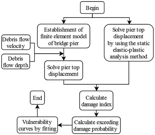
Large-scale infrastructure construction continues in the western region of China, and the highway construction task in mountain areas is huge and arduous. A distinctive feature of highway in mountain areas is the large proportion of bridge, especially the simple-supported and continuous beam bridge with small and medium-sized span. Additionally, after Wenchuan, Yushu, Ludian and Jiuzhaigou earthquakes, the aftershock kept up for a long time, resulting in the loosening of the mountain strata, increasing the probability of debris flow in rainier areas, which may cause major casualties and property losses. The progress of structural analysis and the continuous innovation of engineering building materials has gradually improved the resilience of highway and bridge structures. Although the number of casualties has been already reduced, the social and economic losses are increasing. Accurate hazard risk assessment for hazard prevention and hazard relief is particularly significant. Therefore, the quantitative analysis of the vulnerability of the bridge structure is of great value and significance for the development of hazard prevention and mitigation measures, improving structural resilience and reducing hazard losses. Following consideration of the uncertainty of the model, the impact force of the debris flow is simulated by a finite element analysis method in this paper. Based on the damage evaluation index and the probability of exceeding damage, the debris flow vulnerability of typical highway bridge substructure is quantitatively analyzed by establishing debris flow fragility curve. The flowchart of the proposed methodology is shown as Figure 1.

Figure 1. The flowchart of the proposed methodology.

2. Research background

2.1. Vulnerability model

Vulnerability models provide valuable information to local authorities, emergency and hazard planners concerning the economic loss related to different intensity scenarios that can be used for cost-benefit analysis of structural protection measures (Fuchs and McAlpin 2005). At present, there are two models for vulnerability assessment expressing the vulnerability of buildings to debris flow and the corresponding model uncertainty (Eidsvig et al. 2014). The first model based on structural loss is the main direction and means of the current research, in which the structure loss rate is defined as a ratio of the value (or cost) of loss to its original value. The original value of the structure is estimated by the construction cost, and the value (or cost) of loss mainly access to government agencies, commercial insurance companies, and other public welfare institution. The second model based on damage probability of the structure, namely under the condition of different debris flow intensity, structure reach or exceed the probability of a damage level, in order to achieve the purpose of quantifying the vulnerability of the damaged body. The model incorporates uncertainty implicit, and for each intensity, the curve describes the probability of exceeding certain damage (or probability distribution of damage) rather than a single value of loss degree.

Natural disasters have not been included in the compensation category of commercial insurance in China, and government or research institutes often lack uniform calculation standards when measuring buildings damaged by disasters. Therefore, the first method cannot be applied to the assessment of debris flow losses in China, and the second evaluation model is adopted in this study.

2.2. Forms of debris flow destruction to highway bridge

In order to reduce the loss in the occurrence of debris flow, most of the roads in the debris flow area use bridge structure to cross the debris flow gully to avoid direct flooding of roads and blocking traffic. Therefore, debris flow damage to highway bridges is mainly caused the substructure, which can be summarized as impact, abrasion, scouring and vibration.

(A) Impact: The impact of debris flow is mainly divided into the impact of debris flow slurry and the impact of large stone. The debris flow is a high-density viscous liquid with a large bulk density, often carrying large stones. When debris flow breaks out, the velocity of flow is larger, so it has a greater impact force, which is the main cause of damage to highway bridges.

(B) Abrasion: When flowing along the groove or slope, the debris flow carries a lot of sediment, stone chip and stone fragments, which will strongly abrade the substructure of the highway bridge, especially the pier surface and the collar beam surface. As a result, the protective concrete layer of the pier structure is detached and the steel bar is exposed, which affects the structural safety seriously.

(C) Scouring: The scouring of debris flow to the bridge can be divided into the lower cut of the upstream section, side erosion of the middle section, and the local erosion of the downstream section. Due to scouring, the base level of the abutment in debris flow ditch is lowered and the foundation is exposed, which has a serious influence on the structure.

(D) Vibration: The vibration of the debris flow is very strong, especially the viscous debris flow under high-speed flow, whose shock load is in the form of a pulse, and the most typical waveform is the saw tooth type. This vibration will cause cracks in the bridge structure, reducing its critical intensity, and increasing its probability of damage.

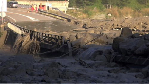
It should be noted that although mainly affects bridge substructure when debris flow reaches a certain volume, another form of damage will occur, that is buried damage, as shown in Figure 2. This form of damage will destroy the bridge deck structure, and inevitably cause road interruption, independent of the debris flow intensity and the probability of damage, so buried damage is not the scope of this study.

Figure 2. A debris flow in the Alps occurred in Bondo village, Glaubinden, Switzerland, on 23 August 2017.

Debris flow often occurs suddenly and fiercely. Among the above five forms of destruction, the impact force is the primary form of damage to highway bridges. The abrasion and scouring action affect the bridge structure repeatedly, which is a long-term destruction process and it will not result in damage to the bridge within a short time. The vibration will increase the probability of damage to the bridge structure to some extent, but it will not lead to structurally damaged directly. Buried damage will inevitably cause road interruptions, therefore, this paper takes impact as the main damage mode, to analyze the vulnerability of typical bridge substructure under debris flow.

2.3. Model uncertainty

Risks and uncertainties associated with civil engineering are crucial to engineers, who can deal with by ignoring, being conservative, using the observational method, or quantifying (Christian 2004). In engineering practice, both aleatory uncertainty and epistemic uncertainty often exist. The former is a kind of contingency with uncertainties expressed by events in a set of probabilistic events. It is accidental, but it has its inevitability. The latter is mainly due to a lack of knowledge, which can be eliminated if we acquire sufficient knowledge about the subject of study. Since epistemic uncertainty can be reduced as knowledge increases, it can also be called reduced uncertainty.

Uncertainty is associated with the input, procedure, and output of the model. For vulnerability models, the input could be qualitative (described with language related to the state and degree of change of things), semi-quantitative (described as classification or level) or quantitative (described as a dimensionless number between 0 and 1, Consortium MOVE 2010). In this paper, only quantitative models are considered.

Various factors related to the vulnerability of debris flow, for instance, house loss rate, debris flow velocity and debris flow depth, the degree of property loss in the building and damaged house height. Therefore, the uncertainty of the vulnerability model cannot be taken into account in an independent factor. In previous studies, the quantification of model uncertainty was not explicitly included or the effect of model uncertainty had been seriously underestimated, even ignored. (Whitman 2000). In this paper, quantitative methods are used to assess the uncertainty of vulnerability rather than qualitative or semi-quantitative methods, so as to provide decision-makers with a tool to identify uncertainty and inquiry into the relationship between risk strategies and actions.

2.4. Construction method of fragility curve

In debris flow area, bridge at different locations is damaged to varying severities. The distribution of damage index can be estimated by the intensity of the debris flow. In order to apply the vulnerability model of probability analysis, Eidsvig et al. (2014) expressed the vulnerability curve as an exceeding damage probability function. The numerical methods for establishing this curve are as follows:

1. Select the damage index and define damage levels relevant to the actual damage.

2. Re-range data on debris flow intensity and damage levels into a damage distribution matrix, and show the number and probability of each intensity interval and damage level.

3. Calculate the probability of exceeding damage for each intensity interval of the current damage state.

4. Fit a fragility curve expressed by the following equation to the data of exceeding damage probability as a function of debris flow intensity. (1) $$P=\raisebox{1ex}{$1$}\!\left/ \!\raisebox{-1ex}{$(1+e^{kI+c})$}\right.$$(1)

Where P is the exceeding damage probability of the structure, I is the intensity of debris flow, k and c are the constant, which can be solved by curve fitting. However, other types of functions are also possible.

3. Related parameter preparation

3.1. Damage index selection

The first step in constructing fragility curves is to select a damage index and define damage levels. The damage evaluation index is a quantitative description of the damage level and a reasonable definition of various damage states. At present, widely used indexes of highway bridge substructure damage are the material strain, the pier top displacement, the curvature ductility ratio, the displacement ductility ratio, and the capacity demand ratio (Hwang et al. 2000). In the seismic response analysis, it was found that for the high pier bridge (the pier height >40 m), the maximum displacement of the pier top does not occur synchronously with the curvature of the most unfavourable section. When the displacement of the pier top reaches its maximum value, the damage of the pier body is not the most serious. There is not a one-to-one correspondence between displacement and damage (Li et al. 2005). Therefore, the strain index and ductility ratio index are commonly used for damage assessment of high pier bridge. The index of capacity demand ratio needs to find the structure's capacity and actual demand for a certain degree of disaster. Its calculation is more complex and less used.

In this paper, the commonly used 20 m height pier in China is selected as the research object. Considering the structure studied in this paper does not involve reciprocating vibration and the dissipation of hysteretic energy is not obvious, this paper simplifies the original Park-Ang index (Park and Ang 1985) and omits one of the cumulative energy dissipation items. It is found that the transverse displacement of the pier top can directly reflect the deformation degree of the structure. Therefore, in the subsequent calculation, the displacement of the pier top is selected as the calculation parameter of damage index, and the following equation is used to calculate and classify the damage degree of the bridge structure. (2) $$D=\frac{{\Delta }_{\text{max}}}{{\Delta }_u}$$(2) where Δ_max is the ultimate displacement of the pier top under the impact force of a certain intensity of debris flow, and Δ_u is the allowable displacement of the pier top.

Originally, 10 damage states with equal interval sizes were defined: 0–0.1; 0.1–0.2; … and 0.9–1. However, due to a few data for some damage index, the corresponding damage states are merged, namely, a larger interval size is used. The interval size 0.1 is kept for damage states up to 0.3 or 0.4 in order to not make the span of the interval too large compared to the damage it represents. Referring to the damage state described by the Park-Ang index, the damage state in this paper is divided into five levels, including non-damage, minor damage, moderate damage, severe damage, and collapse. The relationship between the state description of each damage characteristic and the quantification of the damage index is shown in Table 1.

Table 1. Damage characteristic description and damage quantitative indexes.

Damage state	Damage feature state description	Damage index (D)	Damage level
No damage	Minor local damage	D ＜ 0.1	Level 1
Minor damage	Minor damage is widespread	0.1≤D ＜ 0.25	Level 2
Moderate damage	Severe cracking or peeling of protective layer	0.25≤D ＜ 0.4	Level 3
Severe damage	Concrete crush or longitudinal bar damage	0.4≤D ＜ 0.8	Level 4
Collapsed	Pier fracture	D ≥ 0.8	Level 5

3.2. Bridge substructure sample and finite element model

In order to simulate the impact force of the debris flow and calculate the displacement of the pier top, the sample bridge substructure in this study needs to be confirmed. Shi (2013) conducted a survey on the types of expressway piers in Guizhou, Chongqing, Fujian, Hunan and other provinces in China. Among the 201 sample piers <40 m in length, 156 double column solid piers account for 77.6% of all sample piers. They are the main form of piers below 40 m, and often used in pre-stressed concrete structures. The T-section beam or box-section beam can be selected for the superstructure, and continuous structure or simple support structure can be utilized also. The span is usually 20–40 m. It is commonly used in the construction of highways in China. This paper takes the double column pier shown in Figure 3(a) as an example to discuss the vulnerability characteristics and laws of the substructure of the bridge under the debris flow.

Figure 3. Diagram of double column pier and finite element model. (a) Diagram of double column pier (cm). (b) CSIbridge finite element model.

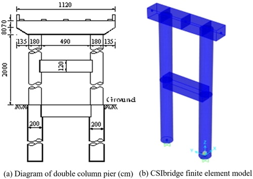
The height of the double-column pier selected in this paper is 20 m, and the pier is a circular section with a diameter of 1.8 m. The length of the cover beam is 11.2 m, of which the height of the middle section is 1.5 m, the width is 2.2 m, and the end is in variable cross-section. The collar beam is positioned in the middle of the pier, which is 1.8 m high and 1.5 m wide, and the bottom is 10 m above the ground. The pier, cover beam, and collar beam are all C30 concrete, and the elastic modulus is 3 × 10⁷ kPa. The longitudinal reinforcement is HRB335, whose ratio of the pier is 1.2%, and the hooping ratio is 0.5%. The finite element analysis is carried out by using CSI-bridge which is a structural analysis and design software (Computers and Structures, Inc. 2013).

Generally, when analyzing the vulnerability of piers, only cantilever pier elements are needed to establish. Although some scholars have established a model that integrates piers, abutments, and superstructure, most of the models are based on consolidation method and do not need too much special treatment for the simulation of the pier bottom boundary. Elastic three-dimensional beam element simulation is adopted in this paper, and the situation of the pile bottom hinge or semi-solid half hinge is not considered. The bridge pier is consolidated with the ground and the pier top is rigidly connected with the cover beam. The finite element model is presented in Figure 3(b).

3.3. Allowable transverse displacement of bridge pier top

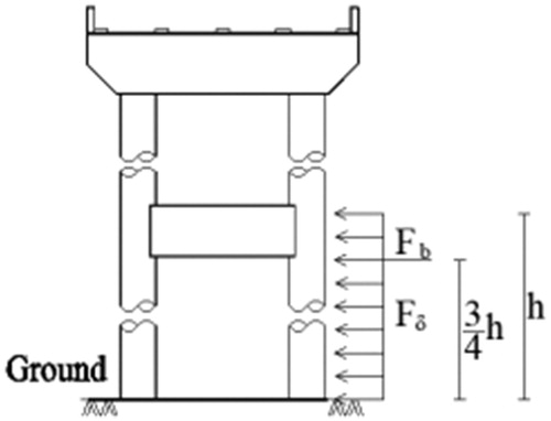
Considering that bridge structures often cross the debris flow gully directly, the impact force of the debris flow is usually perpendicular to the pier surface, which is also the most disadvantageous condition. The damage index established in Section 3.1 needs to calculate the allowable transverse displacement of the pier top of the sample bridge substructure. Chinese highway bridge seismic code (Tang et al. 2008) stipulates that transverse allowable displacement of the double pier can be obtained by using the static elastic-plastic analysis method. Namely, put a horizontal force F in the cap beam, when any of the plastic hinge points of the pier reach the maximum allowable turning angle, cap beam lateral horizontal displacement is the allowable displacement, as shown in Figure 4. The specific calculation process is as follows:

1. Establish a pier model, and configure reinforcement. It is also possible to remove the excess part directly in a full bridge model and retain the constitutive relationship of the material.

2. Set the main control data. The first step is to add the superstructure load. That is, to consider the nonlinear structural analysis under the initial dead load. The second step is to set the horizontal structural thrust F. Since the later analysis adopts displacement control, so the horizontal thrust of this step can be arbitrarily assigned.

3. Define the plastic hinges. The hinge points of the bridge structure generally refer to bending moment hinge. In this case, eight plastic hinge points are set, as shown in Figure 4.

4. Set load conditions. In this case, the initial working condition is the superstructure load and the self-weight of the piers, and relay working condition is the horizontal thrust.

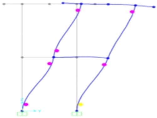
5. Read the structure displacement. The CSI-bridge software uses different colours to represent the state of the plastic hinge (as shown in Figure 5, pink represents the yield condition and yellow for the limit state). Viewing the limit rotation of each plastic hinge at each step. When any plastic hinges at limit state (appear yellow), read the lateral displacement of the pier top in this step.

Figure 4. Schematic diagram of static elastic-plastic analysis and loading of bridge pier.

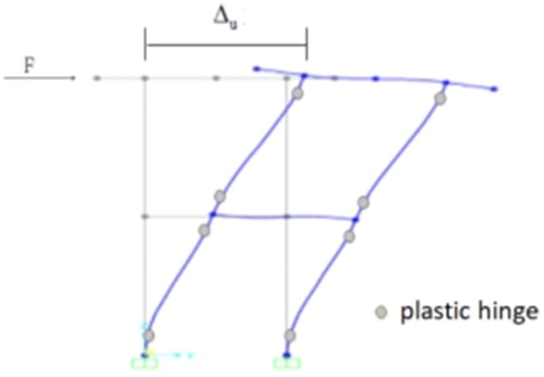
Figure 5. Structural deformation at the limit state of plastic hinge.

According to the above steps, the allowable transverse displacement of the pier top calculated in this example is 0.2107 m.

3.4. Calculation formula and parameters of debris flow impact

As mentioned earlier, the impact of debris flow on the bridge pier is divided into the overall impact of slurry pressure and the impact of the large stone. By adopting the idea of quasi-static equivalent impact load, the overall impact of slurry pressure can be simplified as the pier surface uniformly distributed load, and the impact of the big stone can be simplified to a concentrated load, as shown in Figure 6. The specific calculation Eqs. (3)(3) $$F_{\delta }=\lambda \frac{{\gamma }_c}{g}{\mathrm{v}}^2\hspace{0.17em}\text{sin}\hspace{0.17em}\alpha$$(3) and (4)(4) $$F_b=\sqrt{\frac{3EJ{V}_{\mathrm{s}}{}^{2}W}{g{L}^3}}\hspace{0.17em}\text{sin}\hspace{0.17em}\alpha$$(4) come from the code for design of debris flow resistance of China (China Geological Survey Bureau 2004). (3) $$F_{\delta }=\lambda \frac{{\gamma }_c}{g}{\mathrm{v}}^2\hspace{0.17em}\text{sin}\hspace{0.17em}\alpha$$(3) (4) $$F_b=\sqrt{\frac{3EJ{V}_{\mathrm{s}}{}^{2}W}{g{L}^3}}\hspace{0.17em}\text{sin}\hspace{0.17em}\alpha$$(4)

Figure 6. Schematic diagram of debris flow impact force.

In the equations, F_δ is the overall impact pressure (kPa) of the debris flow, ${\gamma }_c$is the volume-weight of debris flow (kN/m³), v is the velocity of debris flow (m/s), g is the gravity acceleration, α is the angle between the loading surface of the building and the direction of the debris flow stamping (degree), and λ is building shape factor, for example circular building is 1.0, rectangular building is 1.33, square building is 1.47. F_b is impact force of large stone (kN), E is engineering component modulus of elasticity (kPa), J is inertia moment of the central axis of the engineering component section (m⁴), L is the length of the component (m), V_s is the speed of the large stone movement (m/s), and W is the weight of the large stone (kN). The speed of the large stone in the Eq. (4)(4) $$F_b=\sqrt{\frac{3EJ{V}_{\mathrm{s}}{}^{2}W}{g{L}^3}}\hspace{0.17em}\text{sin}\hspace{0.17em}\alpha$$(4) is solved by the empirical Eq. (5)(5) $$V_{\mathrm{s}}=a\sqrt{d_{\max }}$$(5) deduced by Флейшман and Yao (1986). (5) $$V_{\mathrm{s}}=a\sqrt{d_{\max }}$$(5)

In the above equation, a is a comprehensive consideration of friction coefficient, the proportion of stone, debris flow density and basin slope of constant, whose usually value is 3.5–4.5, an average is 4.0. d_max is the diameter of the large stone (m). Assuming that the large stone in the debris flow is granite with a density of 2800 kg/m³ and the average diameter is 1 m, the velocity of the large stone is 4 m/s by Eq. (5)(5) $$V_{\mathrm{s}}=a\sqrt{d_{\max }}$$(5) . The impact force of the large stone is calculated as 521.24 kN according to Eq. (4)(4) $$F_b=\sqrt{\frac{3EJ{V}_{\mathrm{s}}{}^{2}W}{g{L}^3}}\hspace{0.17em}\text{sin}\hspace{0.17em}\alpha$$(4) .

The loading surface of the sample pier is not large compared with that of the large stone, and according to the result of researched by Hu et al. (2006), the large stone in the debris flow is semi-floating movement. Therefore, it is assumed that only one big stone act on the pier at the same time and three-quarters of the debris flow depth is selected as the loading position of the large stone concentrated force, as shown in Figure 6.

4. Construction of debris flow vulnerability model

4.1. Displacement of pier top under different load conditions

For the impact force of the debris flow, the velocity (v) and the depth (h) are important physical indexes and important parameters. According to the previous site investigation of debris flow (Yu and Tang 2016), the velocity of the debris flow in this paper is set as 1, 2, … 15 m/s in total fifteen working conditions, the depth of the debris flow is set as 2, 4, 6,… 20 m in total 10 kinds of working conditions, and a total of 150 working conditions are simulated in this study. At the same time, assuming that density of debris flow is 2100 kg/m³, and inertia moment of the central axis of the cross section is taken as 1.03. The overall impact pressure (F_δ) of the debris flow is obtained by Eq. (3)(3) $$F_{\delta }=\lambda \frac{{\gamma }_c}{g}{\mathrm{v}}^2\hspace{0.17em}\text{sin}\hspace{0.17em}\alpha$$(3) , and the impact force (F_b) of the large stone is 521.24 kN calculated by Eqs. (4)(4) $$F_b=\sqrt{\frac{3EJ{V}_{\mathrm{s}}{}^{2}W}{g{L}^3}}\hspace{0.17em}\text{sin}\hspace{0.17em}\alpha$$(4) and (5)(5) $$V_{\mathrm{s}}=a\sqrt{d_{\max }}$$(5) , which are all working together on the finite element model. The ultimate displacement of the pier top under numerical simulated 150 working conditions can be obtained, as shown in Table 2.

Table 2. Ultimate displacement of pier top under different conditions.

	Velocity (m/s)
Depth(m)	1	2	3	4	5	6	7	8	9	10	11	12	13	14	15
2	0.0002	0.0002	0.0003	0.0003	0.0004	0.0005	0.0006	0.0007	0.0009	0.0010	0.0011	0.0012	0.0014	0.0016	0.0018
4	0.0005	0.0007	0.0009	0.0013	0.0018	0.0024	0.0031	0.0039	0.0049	0.0058	0.0071	0.0083	0.0096	0.0111	0.0127
6	0.0009	0.0014	0.0022	0.0033	0.0048	0.0066	0.0087	0.0112	0.0139	0.0171	0.0204	0.0254	0.0283	0.0327	0.0378
8	0.0017	0.0028	0.0042	0.0071	0.0112	0.014	0.0184	0.0232	0.0291	0.0363	0.0397	0.0471	0.0550	0.0640	0.0732
10	0.0023	0.0041	0.0071	0.0112	0.0161	0.0233	0.0315	0.0393	0.0496	0.0617	0.0742	0.0879	0.1027	0.1188	0.1360
12	0.0033	0.0068	0.0113	0.0176	0.0254	0.0341	0.0467	0.0594	0.0744	0.0912	0.1179	0.1396	0.1633	0.1889	0.2162
14	0.0045	0.0083	0.0142	0.0238	0.0342	0.0482	0.0642	0.0836	0.1041	0.1283	0.1574	0.1856	0.2178	0.2525	0.2894
16	0.0052	0.0113	0.0192	0.0311	0.0461	0.0644	0.0862	0.1127	0.1411	0.1731	0.2162	0.2356	0.2802	0.3186	0.3664
18	0.0063	0.0135	0.0234	0.0354	0.0527	0.0742	0.0993	0.1282	0.1622	0.1995	0.2394	0.2837	0.3328	0.3858	0.4417
20	0.0081	0.0157	0.0287	0.0457	0.0682	0.0954	0.1287	0.1653	0.2085	0.2567	0.3083	0.3672	0.4276	0.4961	0.5683

Jakob et al. (2012) compared the rate of debris flow loss with the four indicators of debris flow which are velocity (v), depth (h), v²h, and vh², and concluded that v²h is most suitable to represent the intensity of debris flow to construct fragility functions. Therefore, v²h is adopted as the index to measure the intensity of debris flow in this paper, and the fragility curve of bridge piers under debris flow is established by using this index as abscissa coordinates. After calculation, 128 different debris flow intensities can be obtained for the above 150 working conditions. The intensity index is denoted by I. The minimum value of intensity is 2, and the maximum is 4500. It should be pointed out that there are 22 identical strength indexes, but the resulting pier top limit displacements are not the same.

After obtaining the ultimate displacement of the pier top under 150 working conditions, the damage index D can be obtained by Eq. (2)(2) $$D=\frac{{\Delta }_{\text{max}}}{{\Delta }_u}$$(2) . The damage indexes can be classified according to Table 1. There are 66 no damage conditions, 22 minor damage conditions, 17 moderately damage conditions, 20 severely damage conditions, and 25 collapsed conditions. Among them, 14 conditions with the debris flow intensity >2500 have all collapsed, so we focus on the study of the rest 136 working conditions of debris flow intensity between 0 and 2500.

4.2. Damage distribution matrix

The data on debris flow intensity and damage level for bridge substructure are re-arranged into a damage level distribution matrix by every 50 intervals of intensity. The number of damage levels generated by different debris flow intensity and their corresponding probabilities can be obtained, as shown in Table 3. The number outside the brackets is the number of corresponding damage levels caused by the intensity of debris flow in this interval, and the number inside the brackets is the probabilities that the intensity of this interval will produce different levels of damage. For example, for an intensity (v²h) of 351–400, a total of 4 working conditions are within damage level 1, accounting for 67%; 1 working condition is within damage level 2, accounting for 17%; 1 working condition is within damage level 3, accounting for 17% too. For intensities less than 150, all the damages are within level 1, that is the v²h of debris flow is <0.1. For intensities higher than 2300, all the damages are within level 5.

Table 3. Damage levels and probabilities of different debris flow intensity interval.

Debris flow intensity	Damage level 1 (P1)	Damage level 2 (P2)	Damage level 3 (P3)	Damage level 4 (P4)	Damage level 5 (P5)
0–50	20 (1)
51–100	12 (1)
101–150	7 (1)
151–200	6 (0.75)	2 (0.25)
201–250	2 (0.5)	2 (0.5)
251–300	4 (0.57)	3 (0.43)
301–350	2 (0.5)	2 (0.5)
351–400	4 (0.67)	1 (0.17)	1 (0.17)
401–450	1 (0.33)	1 (0.33)	1 (0.33)
451–500	2 (0.5)		2 (0.5)
501–550		2 (1)
551–600	2 (0.5)	1 (0.25)	1 (0.25)
601–650		1 (0.33)	2 (0.67)
651–700	1 (0.5)		1 (0.5)
701–750	1 (0.5)			1 (0.5)
751–800	1 (0.25)	1 (0.25)	1 (0.25)	1 (0.25)
801–850			1 (1)
851–900	1 (0.25)	1 (0.25)	1 (0.25)	1 (0.25)
901–950
951–1000		1 (0.25)	2 (0.5)	1 (0.25)
1001–1050		1 (0.5)		1 (0.5)
1051–1100
1101–1150				1 (1)
1151–1200		2 (0.5)		2 (0.5)
1200–1250			1 (1)
1250–1300				2 (1)
1300–1350		1 (1)
1350–1400			1 (0.5)	1 (0.5)
1400–1450				1 (1)
1450–1500				2 (1)
1500–1550
1550–1600			1 (0.5)		1 (0.5)
1600–1650					1 (1)
1650–1700				2 (1)
1700–1750				1 (1)
1750–1800			1 (0.5)		1 (0.5)
1800–1850
1850–1900
1900–1950					1 (1)
1950–2000				1 (0.5)	1 (0.5)
2000–2050				1 (0.5)	1 (0.5)
2050–2100
2100–2150
2150–2200					1 (1)
2200–2250				1 (1)
2250–2300
2300–2350					1 (1)
2350–2400					2 (1)
2400–2450					1 (1)
2450–2500

4.3. Exceeding damage probability

The exceeding damage probability is under a certain intensity of debris flow, structure reaches or exceeds the probability of a certain level of damage, and the calculation method is given in Table 4. From this, the probability of structure exceeding damage in different debris flow intensity intervals can be obtained, as shown in Table 5. It should be pointed out that damage level 5 (collapsed) is the highest level damage, and cannot be surpassed, so there is no sequence of exceeding level 5 damage probability.

Table 4. Calculation methods of exceeding damage probability.

Damage probability	P1	P2	P3	P4	P5
Exceeding damage probability	1 – P1	1 – P1 – P2	1 – P1 – P2 – P3	1 – P1 – P2 – P3 – P4	–

Table 5. Exceeding damage probability under different intensity interval of debris flow.

Debris flow intensity	Exceeding damage probability
	Level 1	Level 2	Level 3	Level 4
0–50	0	0	0	0
51–100	0	0	0	0
101–150	0	0	0	0
151–200	0.25	0	0	0
201–250	0.5	0	0	0
251–300	0.43	0	0	0
301–350	0.5	0	0	0
351–400	0.33	0.17	0	0
401–450	0.67	0.33	0	0
451–500	0.5	0.5	0	0
501–550	1	0	0	0
551–600	0.5	0.25	0	0
601–650	1	0.67	0	0
651–700	0.5	0.5	0	0
701–750	0.5	0.5	0.5	0
751–800	0.75	0.5	0.25	0
801–850	1	1	0	0
851–900	0.75	0.5	0.25	0
901–950	1	1	1	1
951–1000	1	0.75	0.25	0
1001–1050	1	0.5	0.5	0
1051–1100	1	1	1	1
1101–1150	1	1	1	0
1151–1200	1	0.5	0.5	0
1200–1250	1	1	0	0
1250–1300	1	1	1	0
1300–1350	1	0	0	0
1350–1400	1	1	0.5	0
1400–1450	1	1	1	0
1450–1500	1	1	1	0
1500–1550	1	1	1	1
1550–1600	1	1	0.5	0.5
1600–1650	1	1	1	1
1650–1700	1	1	1	0
1700–1750	1	1	1	0
1750–1800	1	1	0.5	0.5
1800–1850	1	1	1	1
1850–1900	1	1	1	1
1900–1950	1	1	1	1
1950–2000	1	1	1	0.5
2000–2050	1	1	1	0.5
2050–2100	1	1	1	1
2100–2150	1	1	1	1
2150–2200	1	1	1	1
2200–2250	1	1	1	0
2250–2300	1	1	1	1
2300–2350	1	1	1	1
2350–2400	1	1	1	1
2400–2450	1	1	1	1
2450–2500	1	1	1	1

4.4. Construction of fragility curve

Approximately take the median value of each debris flow intensity interval in Table 5 as the abscissa and exceeding damage probability as the ordinate. Using Eq. (1)(1) $$P=\raisebox{1ex}{$1$}\!\left/ \!\raisebox{-1ex}{$(1+e^{kI+c})$}\right.$$(1) to fit curve data. The fitting results are presented in Table 6 and the fitting curves are shown in Figure 7. The debris flow fragility curve of sample bridge substructure is shown in Figure 8.

Figure 7. Exceeding damage probability of different levels and their fitting curves. (a) Exceeding damage probability of level 1. (b) Exceeding damage probability of level 2. (c) Exceeding damage probability of level 3. (d) Exceeding damage probability of level 4.

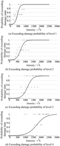
Table 6. Results of fitting exceeding damage probability.

Parameter	Fitting curve of exceeding damage probability
	Level 1	Level2	Level 3	Level 4
K	–0.0122	–0.0083	–0.0061	–0.0034
C	5.5512	5.5624	6.7745	5.8272

4.5. Comparison with existing curves

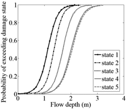
The resulting vulnerability curves proposed in this paper can be compared with other existing curves for debris flows. As mentioned earlier, the model based on structural loss is the main direction and the means of the current research, such as the ones proposed by Luna et al. (2011), Totschnig et al. (2011), Papathoma-köhle et al. (2012), Kang and Kim (2016), and Zhang et al. (2018), as shown in Figure 9. However, there are limited studies based on damage probability of the structure, such as the one proposed by Eidsvig et al. (2014), as shown in Figure 10.

Figure 8. Debris flow fragility curve of sample bridge substructure.

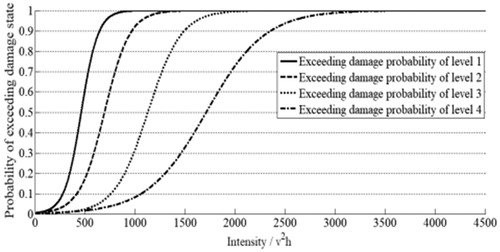
Figure 9. Vulnerability curves based on damage probability.

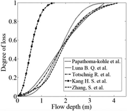
At present, research on the vulnerability curve of debris flow is mostly about the building structure, but the author has not found more research in the field of transportation infrastructure. These studies are all carried out around the building structure, in which the abscissa coordinates are the height of debris flow, not the intensity of debris flow defined in this paper, and the results of vulnerability curves are displayed using different approaches, therefore, a direct comparison has to be carefully interpreted. The vulnerability curves proposed by the above scholars all present the “S” type, and the structural damage increases with the increase of the intensity of the debris flow. The velocity of increase shows the trend of first slow, then fast and last slow, which is consistent with the conclusions drawn in this paper.

The main difference is the slope of the curves. The slope of the curve reflects the resistance of the structure to a certain extent. The larger the slope, the worse the resistance. That is to say, for the same intensity of damage, the larger the slope of the disaster-bearing body, the faster the damage degree increases, and the more vulnerable it is to suffer. This conclusion is confined to the same debris flow, and different debris flows are not applicable due to topography, landform, and types of debris flows.

The vulnerability curve of debris flow based on damage probability of the structure can be used to understand the resistance change of the hazard bearing body from the slope of each curve, as shown in Table 7. Because of the different abscissa, the maximum slope of the curve is altered, but both the results of this study and Eidsvig et al. (2014) show that the slope of each curve presents a downward trend as a whole. That is to say, when the intensity of the debris flow is small, the resistance of the structure is poor, but with the increase of the intensity of debris flow, the resistance of the structure increases, so that it is not easy to collapse. This is very helpful to disaster prevention and control, and the corresponding disaster reduction policies can be formulated according to the characteristics of the structural resistance. Therefore, the author considers that the vulnerability model based on damage probability is superior to the model based on structural loss.

Table 7. Results of fitting exceeding damage probability.

Maximum slope	Exceeding damage probability
	Level 1	Level 2	Level 3	Level 4	Level 5
This paper	0.0029	0.0021	0.0015	0.0008	–
Eidsvig et al. (2014)	1.2819	2.2797	1.0802	0.6457	0.5405

However, unlike the continuous decline of the maximum slope of the fragility curves in this paper, the maximum slope of the curve established by Eidsvig et al. (2014) increases first and then decreases. From this point of view, the vulnerability curve established in this paper is more realistic.

5. Results discussion

5.1. Results analysis

The vulnerability curves shown in Figures 7 and 8 are well fitted with the numerical simulation data, presenting a hypothetical “S” type, which indicates that this is a reasonable hypothesis. With the increase of debris flow intensity, the exceeding damage probability of bridge substructure continues to increase. The shape of each curve is relatively consistent, and the growth at both ends of the curve is slow, and the growth in the middle of the curve is fast, which is in line with the traditional seismic vulnerability curve. As the damage level increases, the debris flows intensity span of each curve increases. Such as the curve of exceeding damage level 1, which intensity of the debris flow is from 0 to 900, and the intensity of the curve of exceeding damage level 4 is from 0 to 3000. That is to say, a higher level of damage requires a higher intensity debris flow. This is more conform to the actual situation.

Figure 10. Vulnerability curves based on structural loss.

5.2. Results application

Quantitative analysis of vulnerability is helpful. It can help us to understand the extent of disaster damage, and it can also be used to fund prioritization by comparing risk estimates associated with different hazard types or for different locations. The debris flow vulnerability model based on this paper can be further applied in the following two aspects:

1. It is possible to calculate the slope of each curve and find out the intensity value with the greatest increase in the slope, which is intensity control point. As shown in Figure 10, when the intensity of the four vulnerability curves in this paper is about 200, 300, 700, and 1200, the slope of the curve increases suddenly, which means that the loss increases suddenly. So these points are the control point of all damage levels. Some effective measures should be taken, such as building protection works, to reduce the intensity of debris flow before it impacts the structure of bridge.

2. The damage probability distribution for a certain debris flow intensity can be obtained, which can help management to better understand the extent of damage caused by debris flow to bridge engineering, to facilitate timely reinforcement and formulate maintenance strategy. The calculation equation is shown in Table 8. Table 9 shows the calculation results when the debris flow intensity is 650 which as an example.

Table 8. Calculation method of damage probability distribution under specific debris flow intensity.

Damage level	Level 1	Level 2	Level 3	Level 4	Level 5
Damage probability	1 – P1(I)	P1(I) – P2(I)	P2(I) – P3(I)	P3(I) – P4(I)	P4(I)

Table 9. Results of the probability distribution of the debris flow intensity at 650.

Damage level	Level 1	Level 2	Level 3	Level 4	Level 5
Damage probability	1 – P1(650) =0.10	P1(650) – P2(650) =0.49	P2(650) – P3(650) =0.36	P3(650) – P4(650) =0.03	P4(650) =0.02

According to the calculation, the probability of damage level 1 is 0.10, level 2 is 0.49, level 3 is 0.36, level 4 is 0.03, and level 5 is 0.02. That is to say, when the intensity of debris flow is 650, of 100 double column pier samples, there are 10 occur level 1 damage, 49 occur level 2 damage, 36 occur level 3 damage, 3 occur level 4 damage, and 2 occur level 5 damage.

The above application is very important for bridge maintenance department. They can take measures to prevent high-intensity debris flow from impacting bridge structure before debris flow occurs. They can also preliminarily judge the disaster situation of bridge structure after debris flow occurs, which provides basis and reference for the next bridge maintenance and reinforcement.

5.3. Model improvement

Admittedly, the vulnerability model proposed in this paper still has some shortcomings, and the improvement of these shortcomings may improve the reliability and results of quantitative analysis in the future. It is, for example, noteworthy that within the 150 working conditions may need further refinement. At the beginning of this study, 150 working conditions were constructed by numerical simulation in order to establish the relationship between the intensity (v²h) of debris flow and the displacement of the pier top. However, the following problems were raised. Firstly, under 150 working conditions, 22 intensity indexes are the same, but the corresponding ultimate displacement of pier top is different. There seems to be no good explanation. Secondly, this paper does not use empirical data obtained from disaster surveys, which reduces the impact of model uncertainty to some extent. But in numerical simulation, a large number of empirical formulas are used. Although these formulas have been verified by many professionals and written into the relevant codes of China, they still add some new uncertainty to the model. This is another drawback of this model.

In order to overcome the above shortcomings, future work can improve the model established in this paper in the following aspects. First, in the simulation of working conditions, the number of working conditions of the debris flow can be further increased, especially the conditions of small-intensity debris flow, which is very helpful for the accurate construction of vulnerability curve. Secondly, in order to obtain more accurate basic data, an equal proportion of the debris flow impact model experiment may need to be implemented. It is believed that the data from this experiment will make the results more accurate.

6. Conclusion

This paper summarized the damage forms of debris flow to bridge substructure. A three-dimensional finite element software is implemented in the preparation of a model for the analysis of typical bridge substructure in China. Based on the exceeding damage probability and the ratio of the ultimate displacements to the allowable displacements of the pier top under different working conditions, the fragility curves of the bridge substructure under the impact of the debris flow is constructed. The following conclusions are achieved in this paper.

1. Debris flow vulnerability curves established in this paper, together with the numerical simulation data show that the S-shaped hypothesis is a sensible assumption, and there is a good fit between the curve and the data. With the increase of debris flow intensity, the probability of damage continues to increase, and it grows fastest in the middle of the curve, which is consistent with the traditional fragility curve.

2. With the improvement of damage level, the debris flow intensity span of exceeding the damage probability of level 1 is from 0 to 900 or so, and the maximum slope is 0.0029, while the intensity span exceeding the damage probability of level 4 is from 0 to 3500 or so, and the maximum slope is 0.0008, that is to say, when the intensity of debris flow is small, the resistance of the structure is poor, but with the increase of the intensity of debris flow, the resistance of the structure increases, so that it is not easy to collapse.

3. The vulnerability curves established in this paper are the same as the existing vulnerability curves, presenting the “S” type. The structural damage increases with the increase of the intensity of debris flow, and the growth rate shows the trend of first slow, then fast and last slow. From the point of view of decreasing the maximum slope of curves with different damage levels, the vulnerability curves established in this paper are more realistic.

4. The vulnerability curve based on the exceeding damage probability established this paper provides the intensity control point and the probability distribution calculation method, which are crucial for the quantification of potential losses. And the Monte Carlo method or other methods can be used to calculate and count probability distribution.

5. At present, there are few kinds of research on the vulnerability of bridge structures under debris flow. The method and application of vulnerability curve model proposed in this paper can provide a reference for vulnerability analysis of highway bridges, and provide the basis for bridge hazard prediction, risk management, and reliability analysis of the traffic system in the future.

Disclosure statement

The authors have no conflict of interest, financial or otherwise.

References

- Akbas SO, Blahut J, Sterlacchini S. 2009. Critical assessment of existing physical vulnerability estimation approaches for debris flows. Proceedings of Landslide Processes: From Geomorphologic Mapping to Dynamic Modeling, Strasbourg, pp. 229–233.
- Bell R, Glade T. 2004. Quantitative risk analysis for landslides-examples from Bíldudalur, NW-Iceland. Nat Hazards Earth Syst Sci. 4(1):117–131.
- Cardinali M, Reichenbach P, Guzzetti F, Ardizzone F, Antonini G, Galli M, Cacciano M, Castellani M, Salvati P. 2002. A geomorphological approach to the estimation of landslide hazards and risks in Umbria, Central Italy. Nat Hazards Earth Syst Sci. 2(1/2):57–72.
- China Geological Survey Bureau. 2004. Design code for debris flow hazard prevention engineering of China. Beijing: China Geological Survey Bureau. pp. 9–15.
- Christian JT. 2004. Geotechnical engineering reliability: how well do we know what we are doing? J Geotech Geoenviron Eng. 130(10):985–1003.
- Флейшман СМ, Yao DJ. (translate) 1986. Debris flow velocity. Debris Flow. Beijing: Science Press; pp. 207–217.
- Computers and Structures, Inc. 2013. CSI Analysis Reference Manual. Berkeley, CA: Computers and Structures, Inc.
- Consortium MOVE. 2010. Methods for the improvement of vulnerability assessment in Europe, guidelines for development of different methods, deliverable D6 in the MOVE project. Chapter 9. In: Eidsvig U, Vangelsten BV, Uzielli M, Welle T, Romieu E, Rohmer J, Ulbrich T, Zaidi RZ, editors. Treatment of uncertainty in vulnerability estimation.http://www.alpaslanhamdikuzucuoglu.com/move-project-move-methods-for-the-improvement-of-vulnerability-assessment-in-europe.html?lang=az.
- Eidsvig UMK, Papathoma-Köhle M, Du J, Glade T, Vangelsten BV. 2014. Quantification of model uncertainty in debris flow vulnerability assessment. Eng Geol. 181((1):15–26.
- Fuchs S, McAlpin MC. 2005. The net benefit of public expenditures on avalanche defense structures in the municipality of Davos, Switzerland. Nat Hazards Earth Syst Sci. 5:319–330.
- Fuchs S, Heiss K, Hübl J. 2007. Towards an empirical vulnerability function for use in debris flow risk assessment. Nat Hazards Earth Syst Sci. 7(5):495–506.
- Huang X. 2015. Study on the vulnerability of debris flow in strong earthquake areas. Dynamic characteristics and quantitative risk assessment of catastrophic debris flows in Wenchuan earthquake-stricken area. PhD thesis, Chengdu University of Technology, Chengdu.
- Hwang H, Jernigan JB, Lin YW. 2000. Evaluation of seismic damage to Memphis bridges and highway systems. J Bridge Eng. 5(4):322–330.
- Hu KH, Wei FQ, Hong Y, et al. 2006. Field measurement of impact force of debris flow. Chinese J Rock Mech Eng. 25(z1):2813–1819.
- Jakob M, Stein D, Ulmi M. 2012. Vulnerability of buildings to debris flow impact. Nat Hazards. 60(2):241–261.
- Kaynia AM, et al. 2008. Probabilistic assessment of vulnerability to landslide: application to the village of Lichtenstein, Baden-Württemberg, Germany. Eng Geol. 101(1–2):33–48.
- Kang HS, Kim YT. 2016. The physical vulnerability of different types of building structure to debris flow events. Nat Hazards. 80(3):1475–1493.
- Li JZ, Song XD, Fan LC. 2005. Investigation for displacement ductility capacity of tall piers. J Earthquake Eng Eng Vibrat. 25(1):43–48.
- Lo W-C, Tsao T-C, Hsu C-H. 2012. Building vulnerability to debris flows in Taiwan: a preliminary study. Nat Hazards. 64(3):2107–2128.
- Luna BQ, et al. 2011. The application of numerical debris flow modelling for the generation of physical vulnerability curves. Nat Hazards Earth Syst Sci. 11(7):2047–2060.
- Luna BQ, Remaître A, van Asch TWJ, Malet J-P, van Westen CJ. 2012. Analysis of debris flow behavior with a one-dimensional run-out model incorporating entrainment. Eng Geol. 128:63–75.
- Luna BQ. 2012. Dynamic numerical run-out modeling for quantitative landslide risk assessment. PhD thesis, University of Twente, Enschede.
- Luna BQ, et al. 2014. Physically based dynamic run-out modelling for quantitative debris flow risk assessment: a case study in Tresenda, northern Italy. Environ Earth Sci. 72:645–661.
- Michael-Leiba M, Baynes F, Scott G, Granger K. 2003. Regional landslide risk to the Cairns community. Nat Hazards. 30(2):233–249.
- Papathoma-Köhle M, Keiler M, Totschnig R, Glade T. 2012. Improvement of vulnerability curves using data from extreme events: debris flow event in South Tyrol. Nat Hazards. 64(3):2083–2105.
- Park YJ, Ang AHS. 1985. Mechanistic seismic damage model for reinforced concrete. J Struct Eng. 111(4):722–739.
- Shi CF. 2013. Calculation and analysis of horizontal displacement on the top of the high piers and a comparison about the pier type in the mountain regions. PhD thesis. Changan University, Xi’an.
- Shinozuka M, Feng MQ, Kim H-K, Kim S-H. 2000. Nonlinear static procedure for fragility curve development. J Eng Mech. 126(12):1287–1295.
- Tang GW, et al. 2008. Seismic design rules for highway bridges. Beijing: China Communications Press; pp. 33–38.
- Totschnig R, Sedlacek W, Fuchs S. 2011. A quantitative vulnerability function for fluvial sediment transport. Nat Hazards. 58(2):681–703.
- Totschnig R, Fuchs S. 2013. Mountain torrents: quantifying vulnerability and assessing uncertainties. Eng Geol. 155((2):31–44.
- Tsao T-C, et al. 2010. A preliminary study of debris flow risk estimation and management in Taiwan. International Symposium Interpraevent in the Pacific Rim, Taipei, pp. 930–939.
- Uzielli M, Lacasse S. 2007. Scenario-based probabilistic estimation of direct loss for geohazards. Georisk. 1:142–154.
- Uzielli M, et al. 2009. Probabilistic risk estimation for geohazards: a simulation approach. International Symposium on Geotechnical Safety and Risk, Gifu, pp. 355–362.
- Whitman RV. 2000. Organizing and evaluating uncertainty in geotechnical engineering. J. Geotech. Geoenviron. Eng. 125(6):583–593.
- Winter MG, Smith JT, Fotopoulou S, Pitilakis K, Mavrouli O, Corominas J, Argyroudis S. 2014. An expert judgement approach to determining the physical vulnerability of roads to debris flow. Bull Eng Geol Environ. 73(2):291–305.
- Xu SB. 2016. Evaluation of vulnerability of subgrade suffering from debris flow hazards. Bull Soil Water Conserv. 36(5):235–241.
- Yu B, Tang C. 2016. Average velocity of debris flow movement. Study on dynamic characteristics and activities of debris flow. Beijing: Science press; pp. 47–64.
- Zhang S, Zhang L, Li X, Xu Q. 2018. Physical vulnerability models for assessing building damage by debris flows. Eng Geol. 247:145.