Changes in river bed terrain and its impact on flood propagation – a case study of River Jayanti, West Bengal, India

Abstract

The investigation of river bed evolution is a principal part of fluvial morphology as it clarifies the procedure of bed deformation and morphological changes on alluvial river bed. Truth be told, the advancement of such bed landscape is additionally accompanied with the regular calamity like flood as it is anticipated due to immense precipitation in Himalayan foot slopes. The flood coverage area is expanding persistently while rainfall homogeneity is acceptable aside from extremely least number of years with sudden precipitation in most recent 101 years. The height of Jayanti riverbed had changed massively in most recent 101 years influencing the idea of channel planform accompanied by huge sediment aggradations and morphological changes which increases the expansion of flood water extension likelihood over bank. It has been discovered through the Fuzzy logic and PCA examination that precipitation does not assume a key job for flood water development yet dynamism of explicit river bed topography prompts bed rise that guarantees the flood propagation of the area unexpectedly.

Keywords:

• River bed terrain
• Evolution
• Flood
• Propagation
• Fuzzy logic

1. Introduction

In India, flow of monsoon rivers permit the unnatural behaviour of channel flow path resulting calamities like flood. Flood is a standout amongst the most unavoidable, unpredictable frequent natural hazard causing severe consequences due to extreme hydrological conditions (Kale 2002; Ahmad and Simonovic 2011). Rivers in foothill of Himalaya regain their 80% flow in monsoon that expresses their hydrological regime along with sediment carrying capacity. During the study, it has been notified that sometime flood propagancy are dignified by not only monsoon rain, but also riverine morphology, especially topographic nature of bed encouraging the water expansion over banks. Unexpected climatic change in the Himalayas because of variation in temperature offers ascend to brisk events of flood (Nandargi and Dhar 2011). It is considered that flood in North Bengal Foothill Rivers are because of unreasonable precipitation in the catchment area (Chakrabortty 2017), however, as stated above, there are numerous other morphological components including sediment transport through channel that engender flood alongside immense measure of precipitation that typically turns into a prime reason for flood each year (Gharbi et al. 2016; Kuo et al. 2017; Lotsari et al. 2018). Understanding the channel morphology in flood studies of the study area is indispensable (Nanson and Croke 1992; Howard 1996; Jain and Sinha 2003; Hooke 2008; Lane et al. 2010). In this investigation site, it has been seen that the idea of precipitation in most recent 101 years is very homogenous in character with the exception of few in some extreme years. In any case, flood probability and expansion of flood water inclusion over the two banks of River Jayanti is expanding in an alarming rate. Jayanti is a perennial river having dynamic water-level characteristics and it gets overwhelmed nearly in each monsoon ensuring harms to damage forest habitat, ecological habitat, human settlements and forest establishments (Das 2009, 2012). After almost every monsoon, the river channel changes its path and widen its planform eroding both the banks vigorously. This disrupts the morphological stability exceeding its geomorphologic thresholds leading to a dynamic fluvial system that tends to adjust its equilibrium condition (Coates and Vitek 1980; Newson 1992; Panniza 1996; Leys and Alan Werritty 1999; Ghosh and Mistri 2012). It brings down overwhelming residue both flaggy and fine comprising Dolomite, limestone, slaty phyllite, calcite and so on, from the Buxa group of Bhutan Hills. Along these lines, constant dregs load that is being conveyed by the stream is deposited in the bed particularly on the chosen investigation zone causing increase in the bed terrain height and diminishing the bank stature. In this study, we have established terrain evolution as a primary cause of flood in river Jayanti (Figure 1), which is a tributary of Torsa and originated from Indo-Bhutan border and situated in the western portion of Kumargram Block of Alipurduar District extending from 26^° 36′00"N to 26^°44′30"N and 89^° 35′30"E to 89^°40′30"E, respectively, covering an area of about 53.73 sq.km. Though hypothetical thinking says that excessive rainfall is a prime cause of flood, but the study reveals a morphological cause that increases the flood propensity which marked the river as flood prone (Das 2012). This paper is concerned about the investigation of river bed terrain evolution in most recent 101 years in a chose stretch of Jayanti River and its effect as far as extension of flood water overbank with time. For the fulfillment of the study in quantitative sense, techniques like principle component analysis (PCA) and the use of Fuzzy Logic has been intended to illuminate the flood stimulation computation of the investigation zone. These two methods have portended the terrain morphological cause dominantly in flood propagation consequences in the area under consideration.

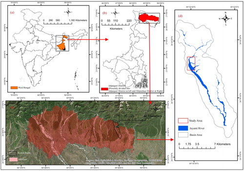
Figure 1. Detail location map of the study area River Jayanti (a–d) showing administrative location details with distinct identified Jayanti River Basin and considered studied stretch of the river. Source: Author (Based on Google Map, SRTM 30m and Toposheet 78F/9, 78F/10 using Arc GIS 10.3.1 platform).

2. Methods

2.1. Riverbed terrain evolution

The terrain evolution process in the most recent 101 years of the Jayanti river bed was obtained using both secondary data and field measurements. Secondary data incorporate Shuttle Radar Topography Mission (SRTM) at a resolution of 1 arc-second (30 m) Digital Elevation Model 2014 and ASTER Digital Elevation Model 2011 from the U.S. Geological Survey for measuring the elevation changes in respective time span. For extraction of contour map, the SRTM Data 2010 and the ASTER DEM 2013 were computed using the Arc GIS 10.3.1 software. As the field measurements were performed for last three years 2016–2018; total station (FOIF, EL302A) survey conducted in the year 2017 at different sections of the riverbed planform were utilized for investigating the recent bed relief of river Jayanti. These data from field were likewise used in creating a contour map on using Arc GIS and TNTmips platform. Furthermore, the contour maps of these three years; 2010, 2013 and 2017 were overlaid which strikingly represents the variation in elevation patterns in terms of values for respective years. GPS (Garmin Oregon 750) was additionally utilized for ground truthing.

The study area is located in a remote location which has nearly lost any economic importance after post-independence and explicitly in the wake of prohibiting of dolomite mining. The stretch of the river chosen for study is the most widest and elevated part of the whole stream. A truss bridge over the river was a standout amongst the most vital imparting components connecting between the village and the mining area. Due to the absence of adequate secondary data, this decay bridge structure which is nearly submerged under the sediments brought down by the river, built in the year 1916 is one of the pioneers in examining the elevation of the riverbed in the last 101 years. Previous study on this area (Ghosh and Saha 2014) has examined the cross section along the bridge from 1993 to 2013 and the measurements of cross section from field survey along the bridge in the year 2017 alongside the height of the bridge provided by the Public Works Department, Jalpaiguri built in the year 1916 clearly proves the elevation changes of the river bed planform. Supporting relevant pictorial images of the bridge as secondary documents have been collected from the local administrative authorities in different time scales. These images have been measured at a scale in respect to the measurement of the remaining decay structure spotted in the field.

Topographical sheet 78 F/9 and 78 F/10 of 1 inch scale, 1929 from National Atlas and Thematic Map Organization (NATMO) was used in preliminary processing of the SRTM data to validate its morphometric attributes like slope map and drainage frequency map created from the SRTM data providing us with an idea of the entire terrain slope and its adjoining tributaries at a glance. The basin boundary was divided into grids of 1 km/1 km scale for grid-wise extraction of various morphometric parameters. Then interpolation of the extracted parameter values from the centroid of each grid was computed using the software’s like Arc GIS 10.3.1 and TNTmips 2013. The long profile of the river has been drawn on the basis of the elevation value obtained from Shuttle Radar Topography Mission (SRTM) 30 m Digital Elevation Model 2014 from the U.S. Geological Survey after error correction at a segment length of 500 m in order to examine its variation in gradient. A graded curve has been drawn on the long profile of the river and its tributaries with the help of the mathematical expression given below (i) $$\mathit{Yc}=a{b}^x+K$$(i) where Y = Altitudinal elevation of the thalweg of the river and its tributaries which is computed as Yc and x = length of the river thalweg.

2.2. Flood propagation

All the rivers in the North Bengal foot hills experience flood almost every year in the monsoon season. Through our study, it has been notified that the rainfall amount in the last 101 years maintains a normal trend. Outrageous precipitation is seen just in couple of years’ rainfall data due to monsoonal characteristics. River Jayanti welcomes flood almost every year. Huge amount of sediment deposition from its tributaries and its sources, specially the finer particles consisting unique characteristics initiates the process of cementation. Cementation leading to change in cross-section area and wetted perimeter of the river (Charlton 2008) further increases flood probability. It rather exceeds the range of flood coverage area threatening human settlement and forest establishments.

The rainfall data of last 101 years were obtained from Atia bari Tea Estate, Kalchini Tehesil, Alipurduar. The data were analysed to find its trend in the last 101 years independent of high flood devastation in the years 1993 and 1998. In relation to explain the overflow expansion of flood water over time, bank height of the river in both sides need to be considered as it acts as a barrier to overbank flow which is distinctly decreasing in nature throughout the time. In this regard, the mean bank height data of 2017 have been collected from the field survey with the help of a staff and a measuring tape. For temporal analysis of bank height, the past bank height data have been collected from qualitative data survey from the local respondents at different time periods. The flood stimulation was computed in Arc GIS Platforms and Global Mapper. The village area being affected due to flood at a water level of 1.73 m was surveyed from the field in July 2017. A digital elevation model was created for two respective years (2011, 2017) from ASTER DEM Data and Total station Survey, respectively. The DEM was prepared using Arc Scene and global mapper 15 platform. The water-level (1.73 m) height surveyed from the field was raised using the software’s mentioned above, to find the stimulation of water in the area. Keeping the water-level constant, flood stimulation was performed on both the DEM (2011 and 2017) pertaining different bed elevation values to analyze its coverage area at the water level of 1.73 m.

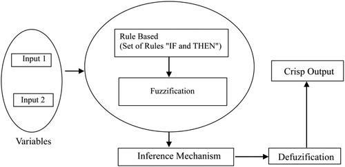
The factor components have also been quantified using a Fuzzy logic binary model using Matlab 15 platform to analyze flood extension in the area studied. The Fuzzy theory proposed by Zadeh (1965) can be summed up in four main parts. First, Fuzification modifies the input into linguistic values which can be further compared to rules. Second, set of rules in rule base controls the system, thirdly, inference mechanism evaluates and fourthly, defuzification provided crisp output (Figure 2) from the conclusion provided by inference mechanism (Nayak et. al, 2005; Kaur and Kaur 2012). The fuzzy logic-based analysis has been designed in respect of five parameters: Bed elevation (be), Bank height (bh), width (w), water level (wl) and depth (d) that initiate flood propagation. These five parameters have been divided into two input membership function sets individually according to its priority. Each input membership function is grouped into three respective classes as mf₁, mf₂ and mf₃ in respect of three considered years, 1916, 1993 and 2017. The degree of membership functions are real and ranges between 0 and 1. All probable Fuzzy relations are drawn between the input and output. Each designed sets have a set of rules in order of “IF and THEN” for each class, respectively that generates a surface view showing its output as flood extension and will help to portray the role of morphological parameters in flood occurrences in this study. If we consider the Fuzzy set as A ranging between [0,1] theoretically, then: $$\left(\forall x\in A\right)\mathrm{ }(A\left(x\right)\in \left[0,1\right])$$ where $A\left(x\right)$ is the membership function of $x$ in A

Figure 2. Schematic representation of the Fuzzy Logic system using Matlab 15.

The flood extension as crisp output values lies between 0 and 1. Here, 0 refers to the least area covered by flood and 1 as the maximum area covered by flood (Van Ranst et al. 1996) with time. If the flood extension value completely belongs to the class than, the membership value is 1, and if not than the membership value is 0. If it to an extent belongs to the class, than the intermediate value will be computed by the S-membership function and can be defined as follows: (ii) $$S\left(x;\mathrm{ }\alpha ,\mathrm{ }\beta ,\mathrm{ }\gamma \right)=\left\{\begin{array}{c}\begin{array}{ll}0;& x\in \left[-x,\alpha \right]\\ 2[(x-\alpha )/(\gamma -\alpha ){]}^2;& x\in [\alpha ,\mathrm{ }\beta ]\\ 1-2[(x-\gamma )/(\gamma -\alpha ){]}^2;& x\in \left[\beta ,\gamma \right]\\ 1;& x\mathrm{ }\in [\gamma ,\mathrm{ }+x]\end{array}\end{array}\right.$$(ii) where$\mathrm{ }\beta =(\alpha +\gamma )/2.$ Here, the complement of the function describes a decreasing membership value (Tang et al. 1991; Van Ranst et al. 1996). In our study, we have considered a three S-membership function as mf₁, mf₂ and mf₃. The rating scale for each parameter’s classes mentioned in Table 1 has been set from both field survey and secondary data. The data for the parameters of the year 2017 were collected entirely from the field observation. For the years 1916 and 1993 were obtained from the images measured at scale and from qualitative data survey from the local respondents at different time periods. Fuzzy rules have been set for rule-based controlling fuzzification and also helping in inference mechanism using “IF and THEN” format. The entire rule for each input set is listed in Table 2. For example: In Bed Elevation (be) and Bank Height (bh), rules has been set as “IF” be is mf₁ and bh is mf₃ then Flood Extension is mf₁ and so on. The inference mechanism further evaluates the input variables with a rule base to defuzzify the set into single crisp value showing a unique value of flood extended area with time in surface viewer. Fuzzy logic using the combination of above-mentioned parameters will portray the significance of the morphological factors in propagation flood mentioning its water-level constant.

Table 1. Flood Extension representing parameters rating scale.

	Flood extension rating scale
Parameters	mf3	mf2	mf1
Bed elevation	180–170.3	174.9–160	160.3–150
Bank height	7.0–4.06	5.516–2.08	2–0.926
Width	500–250	350–200	150–50
Water level	0–2	0–2	0–2
Depth	5–3	4–2	2–0.5

Table 2. Rule set for the parameters in combination.

Input	Rule base	Output
be and bh	(a) if be is mf1 and bh is mf3 than flood extension is mf1	Flood extension
	(b) if be is mf2 and bh is mf2 than flood extension is mf2
	(c) if be is mf3 and bh is mf1 than flood extension is mf3
be and wd	(a) if be is mf1 and wd is mf1 than flood extension is mf1
	(b) if be is mf2 and wd is mf2 than flood extension is mf2
	(c) if be is mf3 and wd is mf3 than flood extension is mf3
bh and wl	(a) if wl is mf1 and bh is mf3 than flood extension is mf1
	(b) if wl is mf2 and bh is mf2 than flood extension is mf2
	(c) if wl is mf3 and bh is mf1 than flood extension is mf3
be and d	(a) if be is mf1 and bh is mf3 than flood extension is mf1
	(b) if be is mf2 and bh is mf2 than flood extension is mf2
	(c) if be is mf3 and bh is mf1 than flood extension is mf3
bh and w	(a) if w is mf1 and bh is mf3 than flood extension is mf1
	(b) if w is mf2 and bh is mf2 than flood extension is mf2
	(c) if w is mf3 and bh is mf1 than flood extension is mf3

Principle component analysis (PCA) is also computed using SPSS for the same number of parameters except depth (data unavailable) for six respective years (1916, 1993, 1998, 2002, 2013 and 2017) to find the most significant factor causing increase in flood coverage area in the study site. PCA is a unique statistical method that converts the interrelated variable to a set of correlated variables computing the maximum weighted component.

3. Results and discussion

3.1. River bed terrain processes in the last 101 years

The terrain evolution for the last 101 years at a cross section has been evaluated from the decayed bridge whose deck is sharing the same ground with the elevated stature of the Jayanti river bed terrain at present. The height of the bridge at the time of its construction in 1916 was 52 feet from its deck. It has been now currently seen that only the decayed supporting towers are visible existence of the bridge over the Jayanti River. Rest of the portion which means 52 ft or 15.85 m is completely submerged under the sediments brought down by the river. This bridge structure clearly reveals that there has been 15.85 m elevation in the height of the river bed including the deck, 0.15 m which has been mentioned as −0.15 m (the deck is considered 0 m) in last 101 years (1916–2017).

SRTM 30 m (2010), ASTER DEM (2013) and the total station data helped us to create a contour map at an interval of 50 m. By overlaying the map of three respective years into a single layout, it is noticed that contour line spacing’s are sifting northwards and an overall increase in bed height by 2017. This also proves the rise of the river bed terrain and thus disrupting its cross section area and its wetted perimeter. The overlaid contour map (Figure 3) reveals the change in contour lines and its shift towards north with respective time period as mentioned. In the year 2017, the brown contour line shows an increase in its height all over the river bed terrain from the year 2010 and 2013. Minute visual observation can state a maximum increase in height at the widest portion of the bed. The isopleth maps (Figure 4) state three individual years 2011, 2014 and 2017 of varied change in elevation in our observed widest part of the river in recent times. Analyzing a particular cross section along the decayed bridge from 1993 to 2017 at respective time period intervals also portrays an increase in its height with time. The cross section was studied for the years 1993, 1998, 2002, 2012 and 2017 which focus on idea of the bed filling in the last 24 years graphically. Thus, graphical representation (Figure 6) clearly depicts the increase of river bed elevation throughout the entire section line. It also portrays the aggradations of sediments towards the left bank of the river at a minor scale in last 24 years which is (Figure 5) clear in the conceptual diagram of the bed filling with time (1993–2017). Figure 7 represents the image of the bridge in 1975, 1993, 1998, 2002, 2013 and 2017 which gives a photographic evidence of the sedimentation width of this particular cross section. In 1975, the bridge was of 11.66 m in height excluding the height of the deck. In 1993, the bridge was 5 m above the river bed floor whereas in 1998, the height of the bridge was only 4.1 m above the Riverbed floor. In 2002, the river bed had been further elevated due to bed filling and the height of the bridge had reduced to 3.5 m. Further in 2013, the height of the bridge had reduced to 0 m or nil which has been further evident to have submerged the deck thus exceeding the initial bridge height. Table 3 shows a change in river elevation from last 101 years and its estimated change every year keeping all factors as constant. Though in real life, uniform state of the controlling factors is not possible. It has been measured that the highest rate of river bed elevation had occurred between 1916 and 2002. This continuous bed filling is a resultant river aggradation process and mostly river is observed to be aggraded towards its left bank between 1993 and 1998 because of huge rate of sediment deposition during the extreme flood in 1993. Thus, the above-explained river bed terrain process in the last 101 years clearly defines 15.85 m of an increase in river bed elevation from the last 101 years.

Figure 3. Superimposition of contour values in three respective years; 2017, 2013 and 2010 at an interval of 50 meter showing the spatio-temporal changes in contour spacing towards upstream. Source: Author (Based on extracted data from SRTM 30m, Aster DEM,Total Station using Arc GIS 10.3.1 and TNTmips platform).

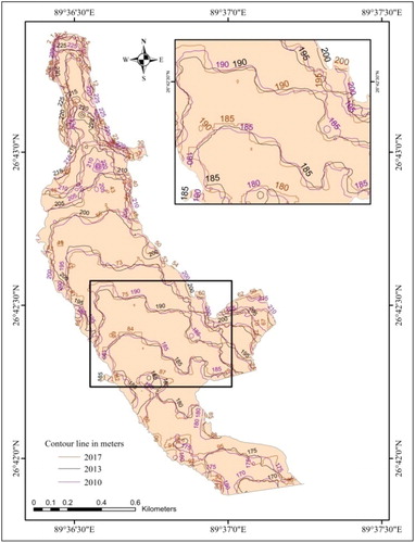
Figure 4. Elevation (m) maps of the riverbed representing topographic variation for three individual years 2011, 2014 and 2017. Source: Author (Based on Data Extracted from SRTM 30m, Aster DEM and Total Station survey using Arc GIS 10.3.1 platform).

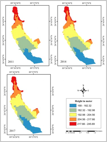
Figure 5. Conceptual diagram of the cross section measured in four respective years depicting increase in bed height (m).

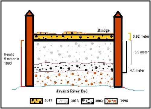
Figure 6. Graphical representation of the cross section considered for showing temporal planform change in five respective years. Source: Pwd office: Jalpaiguri, 2017: self-measured.

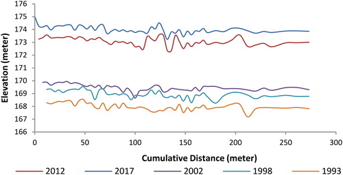
Figure 7. Continuous sediment aggradation resulting riverbed filling and submergence of Jayanti River Bridge with time. (a) Bridge in 1975, (b) 1993, (c) 1998, (d) 2002, (e) 2013, (f) 2017. Source: (a) Local government authority, (b)–(e) Ghosh D., Saha S.; 2013, (f) self-clicked.

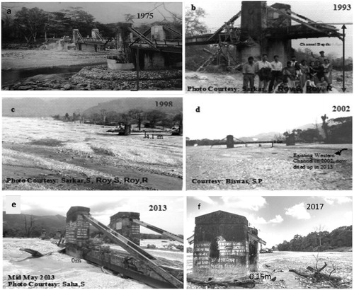
Table 3. Tabular representation of an increase in riverbed height with time along the cross section.

Year	Bridge height from the riverbed (in m)	Change	Interval (in years)	Expected increase in riverbed elevation per year provided all other factors constant (in m/year)
1916	15.85
1975	11.66	4.19	59	0.071
1993	5	0.8	18	0.044
1998	4.1	0.9	5	0.18
2002	3.5	0.6	4	0.15
2013	0	3.5	11	0.05
2017	0.15 (height of the deck)	0.15	4	0.03

3.1.2. Slope and long profile analysis

The Slope map (Figure 8) depicts the nature of the basin slope in degrees ranging between 61.252° and 6.752° and below. The northern and North West part of the map shows a steep slope whereas the southern extent part is under alluvial flat plain. The sudden change in slope after the river gushes down nearly for 2 km downstream from the source area is the major part where aggradation process is continuing in an alarming rate. It is also evident from the long profile (Figure 9) analysis and a distinct break of slope point from where the deposition has started suddenly. The fitted exponential curve (Equation 1(i) $$\mathit{Yc}=a{b}^x+K$$(i) ) that ensure the gradient nature of the channel slope along the river towards the downstream. It is clearly notified that the exponential curve merges with the channel gradient in the concerned point (area from the break of slope till the decayed bridge structure), showing a decrease in value, thus very high rate of deposition. Decrease in channel gradient is prime cause of velocity minimization and an increase in sedimentation overtime.

Figure 8. Spatial differentiation of slope orientation from upstream to downstream of the river.

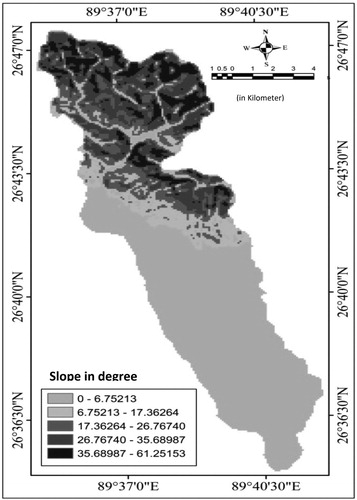
Figure 9. Long profile of River Jayanti portraying the sediment aggradation point near the concerned studied Bridge.

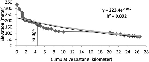
The change in the channel terrain which has been contemplated in regard to River Jayanti has strongly put an impact on the adjoining areas causing flood due to overbank flow. The middle course of the River Jayanti running down from the steep slopes of the Bhutan hills gushes down with high velocity (Ghosh and Saha 2014) and sudden break of slope further helps in the process of huge sediment deposition. The long profile (Figure 9) of the river portrays the break of slope and thus sudden deposition of sediments flattens the channel slope. The river Jayanti studied for the last 101 years (1916–2017) reveals huge deposition of sediments filling up the bed at an alarming rate. Nearly, 15.85 m increase in the height of the bed terrain has completely reformed and reframed the channel in the last 101 years. This entire deforming nature of the river bed terrain that has been analysed from the decayed bridge and field survey measurement values. In every monsoon, the river aggrades huge sediments which do not move downstream in an equilibrium dissemination rate due to its flat channel slope. This occurrence of flow-deposition cycle in every year increases the bed height and decreases the bank height propagating flood.

3.2. Flood propagation

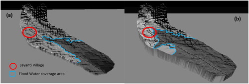
Excessive rainfall in the catchment areas of the Torsa and Raidak-I and II is one of the principle reason causing flood in Jalpaiguri, Alipurduar and Cooch Behar districts (Chakrabortty 2017). Jayanti being a tributary of Torsa River is similarly affected by flood in every monsoon specifically in the month of July and August. The mean monsoon rainfall data for 100 years represented graphically (Figure 10) state a decrease in its rate of mean precipitation with recent time period. The fitted linear line describes the rainfall data homogeneity descending in nature where the value of r² is 0.313 representing normal distribution of rainfall relationship along the foothills. In these regard, the flood propagation and the flood coverage area is increasing with time (Das 2012). Through this work, we have tried to incorporate the channel morphological issues that are acting as a component factor such as riverbed elevation, bank height, width and depth propagating flood. So, as a result, considering the bank height at specific time spans (1993, 1998, 2002, 2013 and 2017) and the height of the water level as constant (1.73 m), we have studied the flood propagation along with increasing scenario of flood expansion area (Figure 11). In 1993, the bank height seems to be 3.24 m and in 1998 it decreases to 2.9 m with the increase of river bed height to 0.34 m. Following this, the bank height of 2002, 2013 had further decreased to 2.17, 1.26, respectively, and 0.96 m in 2017 from the river bed at present. Second, water level as a prime factor of flood has been considered constant to appropriately find the significant role played by the river bed terrain and its continuous elevation propagating flood. The bank height is found decreasing with time initiating flood extending its flood coverage area and is marked as most vulnerable. As a result, the river cross section area has become incapable to hold the same volume of fluid as it could hold in past years before when the height of the bed terrain was much lower and its bank height much higher than what it is at present. This has been further analysed with the flood stimulation on the DEM extracted from Total Station data (2017) and ASTER DEM (2011), respectively. The water level was raised in both the DEM keeping it constant which is 1.73 m (Figure 12). It is observed that the area coverage has exceeded in 2017 (Figure 12b) than in the year 2011 (Figure 12a) increasing its flood water extension area. With a water level of only 1.73 m, the water is observed to have spilled from its wetted perimeter and propagated into the human and forest establishments in 2017. Whereas, with the same water level, 1.73 m, the area covered after the water spill from its planform is less in 2011 than the area observed in 2017. This further proves that increase in river bed terrain height is responsible for flood in the study area rather than the rate of precipitation.

Figure 10. Trend of mean monsoon rainfall in last 100 years (station: Atiabari Tea Estate).

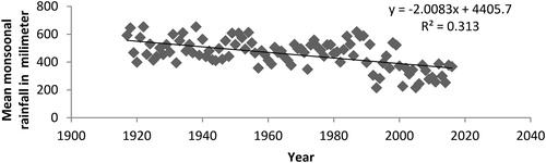
Figure 11. Graphical layout to show a decrease in mean bank height with time in respect of the constant water level (1.73 m).

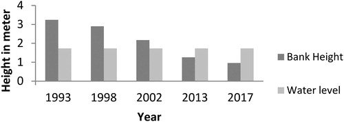
Figure 12. Stimulation of Flood model showing the same water level (1.7 meter) in two respective years; (a) 2011 and (b) 2017 detecting the increased expansion of water coverage due to bed elevation.

The stimulated flood area analysis using Arc GIS has been further clarified by Fuzzy logic binary modeling. As the rainfall data for the last 101 years are homogenous thus other morphological factors such as bed elevation (be), bank height (bh), width (w) and depth (d) has been considered as parameters causing flood in the study area. Here too the water level (1.73 m) observed in 2017 is kept constant like flood stimulation analysis as this vividly explains the significance of the morphological parameters considered in propagating flood in our study area. The combination of be and bh, be and w, be and d, bh and wl, bh and w sets shows a relationship giving a unique value to obtain flood extension, respectively, where, mf₃>mf₂>mf₁ in all the mentioned combinations. Figure 13 is an example of a graphical representation of bank height (bh) as an input variable where S-Membership function where mf₃>mf₂>mf₁. The flood extension as output generates a unique value between 0 and 1. According to the surface view in Figure 14(a) of be and bh, bed elevation (be) is increasing (≤180 m), the bank height (bh) is decreasing (2–0.92 m) resulting the maximum extension of flood whereas, when bed elevation ranging between 140 and 160 m and bank height ≤3.5 m, the overbank flow is observed almost nil. The surface view of be and w (Figure 14(b)) portrays a direct relationship between bed elevation (be) and width (w). As be is increasing, w is also increasing. The third membership function (mf₃) of both shows the maximum extension of flood water. Simultaneously, in combination of be and d (Figure 14(c)), flood water extension is maximum with a decrease in depth and an increase in bed height. Flood extension is maximum when be is mf₃ (180–170.3) and d is mf₁ (2–0.5). This portrays a change in cross section area causing overspill of flood water and increasing its flood coverage area. In combination of bh and w (Figure 14(e)), with a decrease in bank height there is an increase in width. When the bank height is ranging between 0.92 and 2 m, the width is ranging between 500 and 250 m portraying an increase in its coverage area after the bridge was built and changing its width from 86.15 to 338.80 m states an increase in the rivers planform area. As our study signifies the morphological factors as a prime cause of flood water expansion apart from rainfall which is generally a known cause for flood in Himalayan foothills, in combination of bh and wl, the range for wl in all four respective membership functions (mf₁, mf₂ and mf₃) is considered 0–4 m. As water level of a river is a result of rainfall in its catchment area or the area, it is flowing through its range is considered constant in respect of other morphological factors with time. In the surface view of bh and wl, flood extension is increasing with a decrease in bh and decreasing with an increase in its bank height, respectively, with time (Figure 14(d)).

Figure 13. Graphical representation of the S-Shaped membership function (mf₃>mf₂>mf₁) where Bank Height is an input variable.

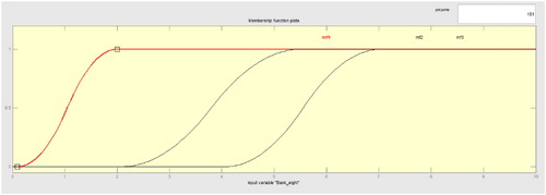
Figure 14. Surface view showing 3-dimensional model of the combinations and flood extension as its output. (a) bed elevation and bank height, (b) bed elevation and width, (c) bed elevation and depth, (d) bank Height and water level and (e) bank height and width as input variables.

PCA is a statistical technique using orthogonal linear combination where the Eigen values are the measures of the explained variance. It finds the most weighted component from the set of variables. PCA for the five parameters already mentioned previously for 6 individual years (1916, 1993, 1998, 2002, 2013 and 2017) states that Bed elevation is one of the most significant components that obtain the maximum weightage with 92.947% variance and Eigen value as 4.649. The Scree plot extracted from IBM SPSS Statistics 23 is shown in Figure 15 portrays the Eigen value in the Y-axis and component value on the X-axis. Table 4 represents the principal component Eigen value and % of variance which further clarify the prime significance of bed elevation in initiating flood propagation. Bank Height also plays a key role in initiating flood with a variance of 5.355% in the second position. The probable cause of not obtaining a Rotated Matrix can be explained as data plotted in one row might be linear combination from the data of other row hence not generating required number of equation as no. of variables.

Figure 15. Graphical representation of the Eigen Value and Component Number in Principle Component Analysis (PCA).

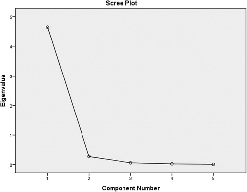
Table 4. PCA showing extraction of Eigen values and % of Variance.

Total variance explained
Component	Initial Eigenvalues			Extraction sums of squared loadings
	Total	% of Variance	Cumulative %	Total	% of Variance	Cumulative %
1	4.649	92.974	92.974	4.649	92.974	92.974
2	0.268	5.355	98.329
3	0.056	1.120	99.449
4	0.022	0.432	99.881
5	0.006	0.119	100.000

Extraction Method: PCA.

Thus, we can outline that irrespective of excessive rainfall, an increase in bed height and an increased volume of water of a cross section of a river can vigorously initiate flood in monsoon. Both flood stimulation, Fuzzy Logic has clarified the significance of the bed elevation playing a prime role in initiating flood and increasing its flood coverage area in our study site including PCA with extracting bed elevation with time as the highest % of variance and Eigen value. The width of the river if noticed in the last 101 year has increased from 86.15 to 338.80 m which also portrays an increase in its planform to nearly 252.65 m with time resulting an increase in its flood coverage area.

4. Conclusion

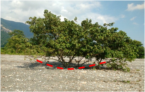
Flood is one of the most uncertain hazards that lead to disaster (Biswas and Banerjee 2018). The study area is affected by flood every year at an alarming rate eroding its manmade artificial banks. Increase in bed elevation at a vigorous rate had almost reached the same ground shared by the village settlement premises that is incorporating the flood water expansion. Village Jayanti and Bhutia Basti are the most affected areas. According to study in 2011, it is found that almost 250 hectors of land is affected (Khalid and Patel 1999; Das 2012) and is increasing unprecedentedly. Sediments and gravels brought down by the river causes decay in plants (Figure 16) as they lose moisture holding capacity resulting physiological drought and siltation due to flood also causes death of plants in huge number (Das 2012).

Figure 16. Submergence of natural vegetation in Jayanti river bed due to sediment and debris aggradation process by the river in monsoon months.

Acknowledgements

The authors convey a token of thanks to the Geography Department, Presidency University, Kolkata. We express our sincere gratitude to Ratnadeep Ray (Former Lecturer at Department of Remote Sensing and GIS, Vidyasagar University, West Midnapore) for his earnest cooperation.

Disclosure statement

No potential conflict of interest was reported by the authors.

Additional information

Funding

This work was supported by the Faculty Research programme and Development Fund for field survey Presidency University, Kolkata.

References

- Ahmad SS, Simonovic SP. 2011. A three-dimensional fuzzy methodology for flood risk analysis. J Flood Risk Manage. 4(1):53–74.
- Biswas M, Banerjee P. 2018. Bridge construction and river channel morphology – a comprehensive study of flow behavior and sediment size alteration of the River Chel, India. Arab J Geosci. 11(16): 1–23.
- Chakrabortty D. 2017. Sit Rep-ii: north Bengal flood report, state inter agency group – West Bengal State, IAG. 1–4. https://sphereindiablog.files.wordpress.com/2017/08/2017-08-17-sitrep-iii-north-bengal-flood.pdf
- Charlton R. 2008. Fundamentals of fluvial geography. London/New York: Taylor and Francis Group/Routledge.
- Coates DR, Vitek JD. 1980. Perspectives on geomorphic thresholds. In: Coates, DR, Vitek, JD editors. Thresholds in geomorphology. London: George Allen and Unwin; p. 3–23.
- Das BK. 2009. Flood disasters and forest villagers in Sub Himalayan Bengal. Economic and Political Weekly. XLIV(4):24–30.
- Das BK. 2012. Losing biodiversity, impoverishment forest villagers: analysing forest policies in the context of flood disaster in a National Park of Sub Himalayan Bengal, India. Occasional Paper. 35:1–2.
- Gharbi M, Soualmia A, Dartus D, Masbernat L. 2016. Floods effects on rivers morphological changes application to the Medjerda River in Tunisia. J Hydrol Hydromech. 64(1):56–66.
- Ghosh S, Mistri B. 2012. Hydrogeomorphic Significance of Sinuosity Index in relation to river instability: a case study of Damodar River, West Bengal, India. Int J Adv Earth Sci. 1(2):49–57.
- Ghosh D, Saha S. 2014. Channel bed aggradation in relation to channel Morphometry: A case study of river Jainti, Jalpaiguri, West Bengal. Int J Geomat Geosci. :192–208. ISSN 0976–4380.
- Hooke JM. 2008. Temporal variations in fluvial processes on an active meandering river over a 20-year period. Geomorphology. 100(1/2):3–13.
- Howard AD. 1996. Modelling channel evolution and floodplain morphology. Floodplain processes. John Willey & Sons Ltd.; Chichester. p.15–53.
- Jain V, Sinha R. 2003. Geomorphological manifestations of the flood hazard: a remote sensing based approach. Geocarto Int. 18(4):51–59.
- Kale V. 2002. Fluvial geomorphology of Indian rivers – an overview. Prog Phys Geog. 26(3):400–433.
- Kaur A, Kaur A. 2012. Comparison of Fuzzy logic and neuro Fuzzy algorithms for air conditioning system. Int J Soft Comput Eng. 2(1):417–420. VolumeIssue-ISSN: 2231–2307.
- Khalid MA, Patel S. 1999. Ecological assessment of habitat loss due to boulder/bed material deposit in rivers of Buxa Tiger Reserve. A Research Report. Department of Forests, Government of West Bengal, 1–4.
- Kuo CW, Chen CF, Chen SC, Yang TC, Chen CW. 2017. Channel planform dynamics monitoring and channel stability assessment in two sediment-rich rivers in Taiwan. Water. 9(2):84–16.
- Lane SN, Widdison PE, Thomas RE, Ashworth PJ, Best JL, Lunt IA, Sambrook Smith GH, Simpson CJ. 2010. Quantification of braided river channel change using archival digital image analysis. Earth Surf Process Landforms. 35(8):971–985.
- Leys KF, Alan Werritty A. 1999. River channel planform change: software for historical analysis. Geomorphology. 29(1/2):107–120.
- Lotsari ES, Calle M, Benit G, Kukko A, Kaartinen H, Hyyppä J, Hyyppä H, Alho P. 2018. Topographical change caused by moderate and small floods in a gravel bed ephemeral river – a depth-averaged morphodynamic simulation approach. Earth Surf Dyn. 6(1):163–182.
- Nandargi S, Dhar ON. 2011. Extreme rainfall events over the Himalayas between 1871 and 2007. Hydrolog Sci J. 56(6):930–945.
- Nanson GC, Croke JC. 1992. A genetic classification of floodplains. Geomorphology. 4(6):459–486.
- Nayak PC, Sudheer KP, Ramasastri KS. 2005. Fuzzy computing based rainfall–runoff model for real time flood forecasting. Hydrol Process. 19(4):955–968.
- Newson MD. 1992. Geomorphic thresholds in gravel-bed rivers—refinement for an era of environmental change. In: Billi P, Hey RD, Thorne CR, Tacconni P, editors. Dynamics of Gravel-Bed Rivers. Chichester: Wiley; p. 1–20.
- Panniza M. 1996. Environmental geomorphology. Amsterdam: Elsevier.
- Tang H, Debaveye J, Ruan D, Van Ranst E. 1991. Land suitability classification based on Fuzzy set theory. Pedologie. XLI-3:277–290.
- Van Ranst E, Tang H, Groenemam R, Sinthurahat S. 1996. Application of fuzzy logic to land suitability for rubber production in Peninsular Thailand. Elsevier, Geodema. 70(1):1–19.
- Yeshewatesfa, H, Bardossy A, Werner HW. 2001. Development of a Fuzzy logic-based rainfall-runoff model. Hydrolog Sci J. 46(3):363–376.
- Zadeh, LA. 1965. Fuzzy sets. Inf. Control. 8(3):338–353. doi: 10.1016/S0019-9958(65)90241-X.