Salinization information extraction model based on VI–SI feature space combinations in the Yellow River Delta based on Landsat 8 OLI image

Abstract

The interference of soil salt content, vegetation, and other factors greatly constrain soil salinization monitoring via remote sensing techniques. However, traditional monitoring methods often ignore the vegetation information. In this study, the vegetation indices–salinity indices (VI–SI) feature space was utilized to improve the inversion accuracy of soil salinity, while considering the bare soil and vegetation information. By fully considering the surface vegetation landscape in the Yellow River Delta, twelve VI–SI feature spaces were constructed, and three categories of soil salinization monitoring index were established; then, the inversion accuracies among all the indices were compared. The experiment results showed that remote sensing monitoring index based on MSAVI–SI₁ with SDI₂ had the highest inversion accuracy (R² = 0.876), while that based on the ENDVI–SI₄ feature space with SDI₁ had the lowest (R² = 0.719). The reason lied in the fact that MSAVI fully considers the bare soil line and thus effectively eliminates the background influence of soil and vegetation canopy. Therefore, the remote sensing monitoring index derived from MSAVI–SI₁ can greatly improve the dynamic and periodical monitoring of soil salinity in the Yellow River Delta.

Keywords:

• Soil salinization
• feature space
• Landsat8 OLI
• monitoring model
• Yellow River Delta

1. Introduction

Soil salinization, currently a global environmental menace, usually occurs in areas characterized by arid climate, great amount of evaporation, shallow groundwater level, and high water-soluble salt content. Salinization critically affects the limited soil resources and results in the deterioration of the regional ecological environment (Allbed et al. 2014; Peng et al. 2018). In addition, the processes of land degradation, such as soil erosion can be triggered by making the ground conditions unsuitable for construction (Fan et al. 2012; Bai et al. 2016). Generally, human-induced activities (the usage of poor quality irrigation water, intense application of fertilizers, and unreasonable cultivation methods) and natural factors (climate change, frequent occurrences of agricultural drought events, and) are the two main driving factors influencing soil salinization (Bouaziz et al. 2011; Allbed and Kumar 2013).

Dynamic and periodical monitoring of soil salinity by knowing when, where, and how salinity may occur is significant for proper management of soil and water resources (Ding and Yu 2014; Fan et al. 2015). However, due to the high spatio-temporal variability, the traditional laboratory analysis methods of characterizing soil salinization cannot provide the dynamic information on a large scale, especially for regions with scare known data (Kumar et al. 2015; El-Battay et al. 2017). Remote sensing techniques have been widely used to assess soil salinity since the 1960s, and they are advantageous, as they allow for ground observations at large spatial scales and high temporal resolutions (Fallah Shamsi et al. 2013; Gorji et al. 2017). Moreover, using these techniques, the spectral information of soil salinization can be obtained repeatedly with short temporal intervals (Gorji et al. 2015; Scudiero et al. 2015). The spectral characteristics of saline soils are theoretical basis for remote sensing monitoring. There is a positive relationship between soil reflectance in visible-near infrared–shortwave infrared bands and soil salinization. However, the dynamic processes occurring at the saline soil interface largely constrain the periodic monitoring of soil salinization (Wu et al. 2014).

Currently, there are two main approaches to obtain the salinization information based on remote sensing images, which are visual interpretation and automated classification considering soil salinity, groundwater, and other auxiliary factors (Khan et al. 2005; Allbed and Kumar 2013). However, quantitative analysis using the above two methods are insufficient because of the influence of human factors (Noroozi et al. 2012). Moreover, most quantitative analysis methods consider only spectral information of bare soil, ignoring the indirect response of vegetation information to salinization (Weng et al. 2010). Several researchers have conducted quantitative studies on soil salinity by utilizing digital indices derived from different spectral bands of satellite images (Wang et al. 2002; Yao and Yang 2010; Zhang et al. 2011; Yahiaoui et al. 2015; Zhang et al. 2015; 2019). The effects of salinization on the characteristics of spectral reflection by acquiring field samples and reflectance by spectrometer were analyzed to identify (Farifteh et al. 2008). Multiple indices comprising of spectral bands in different combinations were calculated and compared to identify salinized soils with a higher degree of accuracy . In addition, it has been found that the scatter plots of vegetation cover and soil moisture appear as a triangle when the variation range of the two parameters is large. The characteristic information of feature spaces has been widely applied to study soil salinity inversion and monitor information of surface evapotranspiration, soil moisture, crop moisture content, and desertification, and beneficial results have been realized (Allbed and Kumar 2013). Moreover, the significant relationship has been confirmed by previous studies. Ha et al. (2009) proposed the Albedo-SI feature space model to monitor the salinization information, which obtained better results. However, the above model did not take the indirect response of vegetation to soil salinization into consideration. Ding et al. (2013) utilized the modified soil adjust vegetation index (MSAVI) and Wetness Index (WI) to construct MSAVI–WI feature space to obtain the salinization index, which ignored the direct salt content of soil. Wang et al. (2010) chose normalized difference vegetation index (NDVI) and SI to establish the model of NDVI–SI feature space, which could better distinguish the spatial distributions of different levels of salinization. However, the comparisons between NDVI and other vegetation indices (VI) were not conducted to select the optimal VI to construct the feature space model. Zhang et al. (2016) also established a model derived from MSAVI–SI feature space to monitor the salinization of Manas River Basin, which, however, ignored the non-linear characteristic between vegetation and salinized soil. Thus, by comprehensively considering the bare soil and vegetation information, the inversion accuracy of soil salinity can be improved.

The objectives of this study are to fully consider the interference of soil salt content, vegetation, and other factors on soil salinization monitoring via remote sensing techniques, and to improve monitoring accuracy, especially for the surface vegetation landscape in Yellow River Delta. These concerns are crucial in remote sensing monitoring of soil salinization. In this paper, different vegetation indices–salinity indices (VI–SI) feature spaces are compared and analyzed to recommend the optimal model for monitoring soil salinization in the Yellow River Delta.

2. Materials and methods

2.1. Study area

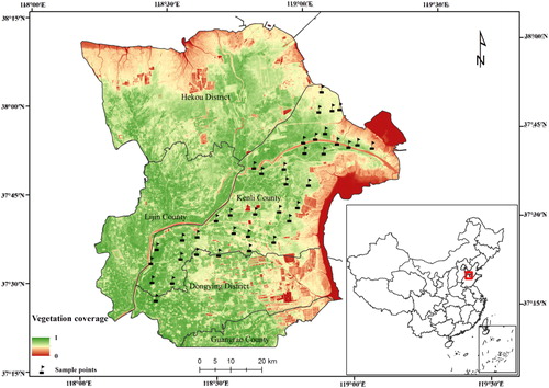
The Yellow River Delta, situated on the northern coast of China (37°20′–38°12′N, 118°07′–119°10′E, Figure 1), encompasses an area of over 6000 km². It is a neoteric delta, which starts from Ninghai and ends at Zimai Stream mouth at southeast, and Taoer River at northwest (Weng et al. 2008). The newly formed wetland extends from the mouth of the Yellow River to the Bohai Sea. The study area has a monsoon climate, which is characterized by average annual temperature ranging from 11.7 to 12.6 °C and average annual precipitation ranging from 530 to 630 mm. The annual average evapotranspiration ratio is 3.22. The groundwater table is relatively high and ranges from 1.6 to 2.4 m, with a mineralization degree of 32.4 g L⁻¹. The saline land covers more than 70% of the total area with the salt content of the soil surface (0–15 cm) ranging f from 0.4% to 1.5% due to the low and flat terrain, heavy seawater intrusion, high ground water table and high ground water salinity. The main soil type is gleyic solonchaks with a high sand proportion and high salinization. The dominant plant species include Suaeda salsa (L.) Pall, Tamarix chinensis Lour., Tamarix ramossisima Ledeb., Suaeda glauca (Bunge) Bunge, and Phragmites australis Trin., which are most commonly salt-tolerant herbaceous plants and shrubs (Zhang et al. 2017).

Figure 1. Location of the study area and spatial distribution of sample points.

2.2. Data collection and preprocessing

A Landsat8 OLI image (August 26, 2016), with a path/row of 121/34, was downloaded from https://glovis.usgs.gov/. The image quality was higher with a total cloud cover of less than 5%. In this study, five spectral bands in visible and infrared wavelengths to calculate typical vegetation and salinity indices—band 2 (blue, 0.45–0.51 µm), band 3 (Green, 0.53–0.59 µm), band 4 (Red, 0.64–0.67 µm), band 5 (NIR, 0.85–0.88 µm), and B7 (SWIR2, 2.11–2.29 µm)—with a spatial resolution of 30 m were utilized. To eliminate the effect of geometric–radiometric distortions and atmospheric perturbations on the image quality, geometrical calibration (to adjust the deviation between image and map positions) and atmospheric correction using the tool of Registration and FLAASH model were performed with ENVI 5.3. On the August 25 and 26, 2016, 160 topsoil samples were collected at a depth of 0–10 cm, which were selected from regions with different soil types and vegetation types. This quadrat (30 m × 30 m), including at least three samples (generally plum blossom shape with five samples) was set with GPS to match the pixel of Landsat8 OLI. There were 26 valid quadrats in this investigation. The sampled top soil was preserved in freshness protection package with different labels. To measure soil salt content, 250 ml distilled water was mixed with different 50 g of processed soil sample. And, the soil salt content of one quadrat was the mean value of those samples in the quadrat.

2.3. Vegetation and salinity indices

The electromagnetic energy that is reflected from targets to obtain information can be utilized to monitor the Earth's surface by remote sensing. Thus, the remotely sensed vegetation reflectance can be used as an indirect indicator of soil salinity because that soil salinity can impact the grown of vegetation. Healthy vegetation has a high reflectance in the near infrared region due to the cellular structure of plant leaves and a low reflectance in the visible region due to absorption by chlorophyll. However, unhealthy vegetation shows an increased reflectance in the visible region and reduced reflectance in the near infrared region because of less chlorophyll in the leaves.

Khan and Sato (2001) found that the red band of ETM + image had a significantly sensitive response to soil salinity. In addition, by comparing the spectral characteristics and band mixing experiments of typical objects, it has been found that the soil salinity indices derived from blue and red bands of remote sensing images can better reflect the information of soil salinization (Scudiero et al. 2015). Moreover, there was a significant positive correlation between the soil salinity indices and field observed salt content. Thus, in the present study, soil salinity indices were selected as a biophysical parameter for monitoring the salinization process.

Salt is one of the most important factors that restrict vegetation growth in soil chemistry (Fan et al. 2015). The type, biomass, and succession characteristics of halophytic vegetation are highly related with soil salt content. Moreover, with increase of salt content in surface soil, the vegetation indices decrease and the soil electrical conductivity increases (Wu et al. 2014). Thus, the vegetation indices can be used as an indirect parameter for discriminating saline soil.

Considering the surface eco-environmental landscape of the Yellow River Delta and related studies, four typical vegetation indices and three salinity indices were selected to construct VI–SI feature spaces (Table 1).

Table 1. Summary of some widely used vegetation and soil salinity indices for soil salinization assessments.

Formulation	Study area	References
$\text{NDVI}=\frac{\text{NIR}-R}{\text{NIR}+R}$	Western San Joaquin Valley, California	Scudiero et al., 2015
$\text{GNDVI}=\frac{\text{NIR}-G}{\text{NIR}+G}$	Dujaila of Iraq	Wu et al., 2014
$\text{MSAVI}=\frac{\left(2\text{NIR}+1\right)-\sqrt{{\left(2\text{NIR}+1\right)}^2-8\left(\text{NIR}-R\right)}}{2}$	Indo-Gangetic plains of India,Wei Gan River, and the Kuche River basin in Xinjiang	Peng et al., 2018; Kumar et al., 2015
$\text{ENDVI}=\frac{\left(\text{NIR}+{\text{SWIR}}_2-R\right)}{\left(\text{NIR}+{\text{SWIR}}_2+R\right)}$	The Yellow River Delta of China	Weng et al., 2008; Fan et al., 2012
${\text{SI}}_1=\sqrt{B\times R}$	The Yellow River Delta of China	Fan et al., 2012
${\text{SI}}_3=\sqrt{G^2+R^2+{\text{NIR}}^2}$	Lower Chéliff plain, Algeria	Yahiaoui et al., 2015
${\text{SI}}_4=\sqrt{G^2+R^2}$	Lower Chéliff plain, Algeria	Yahiaoui et al., 2015

Note: B, G, R, NIR, and SWIR2 refer to blue band, green band, red band, and shortwave infrared band (2100–2290 nm), respectively; ENDVI: enhanced normal differential vegetation index; GNDVI: green normalized difference vegetation index; NDVI: normal differential vegetation index; MSAVI: modified soil-adjusted vegetation index.

2.4. Standardization of indices

To eliminate the differences in magnitude of vegetation indices and salinity indices, the maximum and minimum values for these variables were calculated and were applied in the data standardization process. (1) $$V_i=\frac{{\text{VI}}_i-{\text{VI}}_{i,\text{min}}}{{\text{VI}}_{i,}{}_{\text{max}}-{\text{VI}}_{i,\text{min}}}$$(1) (2) $$S_i=\frac{{\text{SI}}_i-{\text{SI}}_{i,\text{min}}}{{\text{SI}}_{i,\text{max}}-{\text{SI}}_i{}_{,\text{max}}}$$(2) where V_i denotes the normalized vegetation indices i; VI_i denotes the vegetation indices i; VI_i,min denotes the minimum value of vegetation indices i; VI_i,max denotes the maximum value of vegetation indices i; S_i denotes the normalized salinity indices i; SI_i denotes the salinity indices i; SI_i,min denotes the minimum value of salinity indices i; and SI_i,max denotes the maximum value of salinity indices i.

3. Constructions of feature space and remote sensing monitoring model of salinization

3.1. Construction of the VI–SI feature space

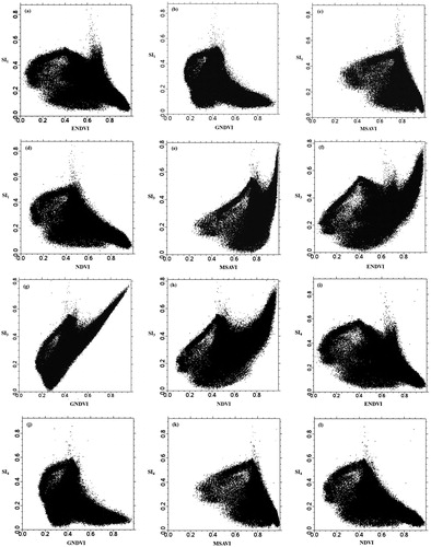
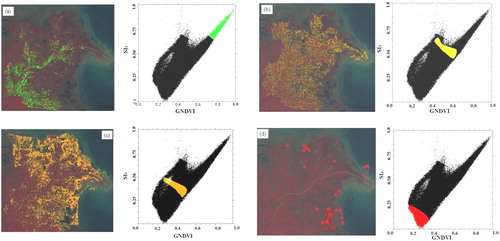
Using the four vegetation indices and three salinity indices, 12 VI–SI feature spaces were constructed. Figure 2 shows that the VI–SI feature spaces can be divided into three categories based on the shape of feature space and the spatial patterns (in the feature space) of different levels of salinized soil. The first category includes Figure 2(a), (b), (d), (i), and (j) while the second category includes Figure 2(e), (f), (g), and (h). In addition, Figure 2(c) and 2(k) belong to the third category. In this paper, NDVI-SI₁, MSAVI-SI₁, and GNDVI-SI₃ were selected to analyze the characteristics of the feature spaces of the above three categories, respectively.

Figure 2. Twelve VI-SI feature spaces: (a) ENDVI-SI₁; (b) GNDVI-SI₁; (c) MSAVI-SI₁; (d) NDVI-SI₁; (e) MSAVI-SI₃; (f) ENDVI-SI₃; (g) GNDVI-SI₃; (h) NDVI-SI₃; (i) ENDVI-SI₄; (j) GNDVI-SI₄; (k) MSAVI-SI₄; (l) NDVI-SI₄.

3.2. Analysis of salinization process in feature space

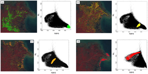
As shown in Figure 3, the spatial distributions of different levels of salinized soil in NDVI-SI₁ feature space (plotted by the tool of ENVI 5.3) differed significantly. The vegetation coverage declined while the salinity increased continuously. According to the distance to the point (1, 0), we chose four point clusters which were distributed in different areas in this study region. Twenty-five field-observed samples for each point cluster were utilized for analysis to investigate the relationship between different levels of soil salinization and four point clusters. The results showed that different levels of salinized soil (non-salinization (<1.0 g kg⁻¹), slight salinization (1.0–2.0 g kg⁻¹), moderate salinization (2.0–4.0 g kg⁻¹), and severe salinization (>4.0 g kg⁻¹)) were located in different areas in the NDVI–SI₁ feature space. Moreover, the process of soil salinization could be better distinguished and was consistent with the field survey results.

Figure 3. Different soil salinization contents in image and NDVI-SI₁ feature space: (a) non salinization; (b) slight salinization; (c) moderate salinization; (d) severe salinization.

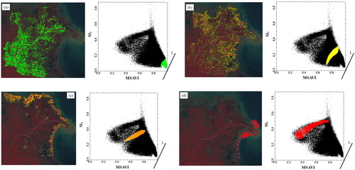
As shown in Figure 4, the spatial distributions of different levels of salinized soil in MSAVI–SI₁ feature space differed significantly. Similar to the perpendicular drought index proposed by Zhang et al. (2009), there also existed L line in the MSAVI–SI₁ feature space, which was perpendicular to the soil line. The distance from any point in the feature space to line L can be utilized to explain the soil salinization process. The farther away from line L, the more serious salinization is. According to the distance to the line L, we also chose four point clusters which were distributed in different areas in this study region. To investigate the relationship between different levels of soil salinization and four point clusters, twenty-five field-observed samples for each point cluster were utilized for analysis and verification. The results showed that different levels of salinized soil (non, slight, moderate, and severe) were located in different areas in the MSAVI–SI₁ feature space.

Figure 4. Different soil salinization contents in image and MSAVI-SI₁ feature space: (a) non salinization; (b) slight salinization; (c) moderate salinization; (d) severe salinization.

According to the distance to the point (1, 1), four point clusters were also selected, and their corresponding areas were distributed in different regions (Figure 5). Then, twenty-five field-observed samples for each point cluster were utilized to analyze the relationship between soil salinization process and four point clusters. The results indicated a better relationship between different levels of soil salinization and point clusters.

Figure 5. Different soil salinization contents in image and GNDVI-SI₃ feature space (a) non salinization; (b) slight salinization; (c) moderate salinization; (d) severe salinization.

3.3. Remote sensing monitoring model of salinization

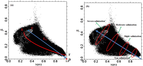
As shown in Figure 6(a), an obvious non-linear relationship existed between NDVI and SI₁, which nearly approximates the trajectory of soil salinization process in the NDVI–SI₁ feature space. The E–F line is the trajectory line of feature space with the start point E and end point F. The straight line perpendicular to the E–F line can distinguish different levels of salinized soils. The distance from any point in the feature space to point D (1, 0) can be used to indicate the soil salinization state; that is, the farther away from point D, the more salt the soil has, and the more serious salinization is. The remote sensing monitoring model of soil salinization (salinization detection index, SDI₁) can be expressed as the distance L₁ from point C (any point in the NDVI–SI₁ feature space) to point D: (3) $${\text{SDI}}_1={\mathrm{L}}_1=\sqrt{{(\text{NDVI}-1)}^2+{\text{SI}}_1{}^2}$$(3) where L₁ refers to the distance from C to D.

Figure 6. Construction of NDVI–SI₁ feature space: (a) model of salinization detection index; (b) distance for different soil salinization levels in NDVI-SI₁ space.

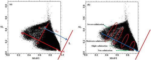
There was an obvious non-linear relationship between MSAVI and SI (Figure 7). The distance from any point in the feature space to line L can be utilized to explain the soil salinization process. The farther away from line L, the more serious salinization is. Taking any point P in the MSAVI–SI₁ feature space and according to the distance formula between point and line, the remote sensing monitoring model of soil salinization (salinization detection index, SDI₂) can be expressed as the distance L₂ from P to line L: (4) $${\text{SDI}}_2={\mathrm{L}}_2=\frac{\left|1-\text{MSAVI}+\mathrm{M}\times {\text{SI}}_1\right|}{\sqrt{{\mathrm{M}}^2+1}}$$(4) where L₂ refers to the distance from point P to line L, the M refers to the gradient of soil line.

Figure 7. Construction of MSAVI–SI₁ feature space (a) Model of salinization detection index (SDI₂); (b) Distance for different soil salinization in MSAVI-SI₁ feature space.

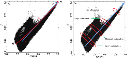
Similar to Figure 6, an obvious non-linear relationship also existed between GNDVI and SI₃ (Figure 8). The straight line perpendicular to the M–N line can distinguish different levels of salinized soils. The distance from any point in the feature space to point O (1, 1) can be utilized to explain the soil salinization process. The farther away from point O, the more serious salinization is. According to the formula for distance between two points, the remote sensing monitoring model of soil salinization (salinization detection index, SDI₃) can be expressed as the distance L₃ from point Q (any point in the GNDVI–SI₃ feature space) to point O: (5) $$\mathit{SD}{I}_3=L_3=\sqrt{{(\text{GNDVI}-1)}^2+{({\text{SI}}_3-1)}^2}$$(5)

Figure 8. Construction of GNDVI-SI₃ feature space: (a) model of salinization detection index; (b) distance for different soil salinization levels in GNDVI-SI₃ space.

4. Results and discussion

Utilizing the above three types of models, the salinization information has been calculated with the tool of Band Math (ENVI 5.3). Then the spatial patterns of different levels of soil salinization have been shown in Figure 9.

Figure 9. Spatial distributions of salinization index for twelve models based on VI-SI feature spaces (a) MSAVI-SI₁; (b) ENDVI-SI₁; (c) GNDVI-SI₁; (d) NDVI-SI₁; (e) ENDVI-SI₃; (f) GNDVI-SI₃; (g) MSAVI-SI₃; (h) NDVI-SI₃; (i) ENDVI-SI₄; (j) GNDVI-SI₄; (k) MSAVI-SI₄; (l) NDVI-SI₄.

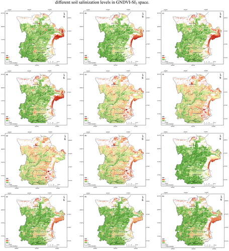
To examine the inversion accuracy of the twelve monitoring models of soil salinization, 26 filed observed samples were utilized (Table 2). As shown in Figure 10, the inversion accuracy of different monitoring modes differed greatly with the R² ranging from 0.719 to 0.876. The inversion accuracy of the MASVI–SI₁ feature space with SDI₂ was the highest, with R² = 0.876, while that of the ENDVI-SI₄ feature space with SDI₁ was the lowest, with R² = 0.719. Overall, the monitoring models based on SI₁ indices had the best mean inversion accuracy (0.842), followed by SI₃ and the monitoring models based on SI₄ had the lowest mean inversion accuracy (0.731). The red band had a sensitive response to soil salinity (Khan and Sato 2001). Moreover, the SI₁ indices derived from blue band and red band could better indicate the salinization process; this has been confirmed by comparing the spectral characteristics of typical objects and the band mixing test analysis (Scudiero et al. 2015). In addition, the monitoring models composed of MSAVI had better mean inversion accuracy (0.817) than those composed of NDVI (0.803). The NDVI was sensitive to changes in soil background. In an area with lower vegetation coverage, NDVI is greatly influenced by soil background and thus can underestimate some vegetation information. However, MSAVI fully considers the bare soil line and thus effectively eliminates the background influence of soil and vegetation canopy (Weng et al. 2008). The mean inversion accuracy of monitoring models composed of ENDVI (0.810) was higher than those composed NDVI (0.803) and GNDVI (0.783). This is because that the ENDVI had considered shortwave infrared band (2100–2290 nm), which could better reflected the influence of soil salt content on vegetation. Therefore, the remote sensing monitoring model based on MSAVI-SI₁ with SDI₂ was the most effective approach to obtain the information of saline soil in the Yellow River Delta.

Figure 10. Comparisons of inversion accuracy for different monitoring modes.

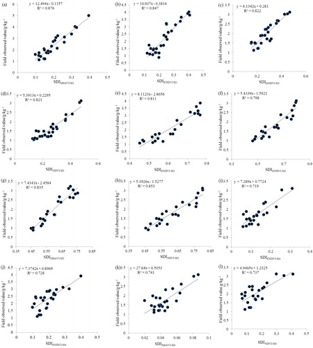
Table 2. Values of measured soil salt content.

Sample number	Measured soil salt content/g kg^−1	Sample number	Measured soil salt content/g kg^−1
F01	3.07	F14	1.74
F02	5.01	F15	1.72
F03	4.031	F16	2.65
F04	1.59	F17	3.97
F05	2.72	F18	1.51
F06	2.82	F19	1.22
F07	3.38	F20	1.22
F08	3.23	F21	1.20
F09	3.12	F22	1.12
F10	2.09	F23	1.89
F11	2.32	F24	1.49
F12	2.14	F25	1.84
F13	1.99	F26	1.41

For different study regions, the sensitive parameters of feature space to monitor the soil salinization differed significantly. In addition, the vegetation response to salinization process is non-linear. Through the comprehensive comparisons among different VI–SI feature space, linear and non-linear models, the optimal model based on MSAVI–SI₁ for the Yellow River Delta was proposed to better improve the above deficiencies than previous studies.

5. Conclusion

Considering the surface eco-environmental landscape of the Yellow River Delta and related studies, four typical vegetation indices (ENDVI, NDVI, GNDVI, and MSAVI) and three salinity indices (SI₁, SI₃, and SI₄) derived from Landsat8 OLI were selected to construct twelve VI-SI feature spaces. Then the optimal monitoring model of salinization for the Yellow River Delta based on VI-SI feature space were proposed by the inversion accuracies comparison among the twelve models with the field sampling data. The results showed that: (1) The relationship between vegetation indices and salinity indices in a feature space can be used to retrieve regional soil salinity information. (2) The remote sensing monitoring index based on MSAVI–SI₁ with SDI₂ had the highest inversion accuracy, with R² = 0.876, while that based on the ENDVI–SI₄ feature space with SDI₁ had the lowest, with R² = 0.719. The reason lied in the fact that NDVI was greatly influenced by soil background and thus can underestimate some vegetation information, while MSAVI could fully consider the bare soil line and thus effectively eliminates the background influence of soil and vegetation canopy. And, SI₁ that composed of blue band and red band was a better biophysical parameter for monitoring the salinization process than other salinity indices. The results further clarify the mechanism and occurrence of soil salinization and therefore provide a scientific basis for the prevention and treatment of soil salinization. However, further studies need to be conducted to clarify the mechanisms underlying the process of soil salinization and strengthen the inversion accuracy.

Disclosure statement

No potential conflict of interest was reported by the authors.

Additional information

Funding

This work was supported by Natural Science Foundation of Shandong Province (Grant Nos. ZR2018BD001); Project of Shandong Province Higher Educational Science and Technology Program (Grant No. J18KA181); Key Research Program of Frontier Science of Chinese Academy of Sciences (Grant No. QYZDY-SSW-DQC007); Open Fund of Key Laboratory of Geographic Information Science (Ministry of Education), East China Normal University (Grant No. KLGIS2017A02); Open Fund of State Laboratory of Information Engineering in Surveying, Mapping and Remote Sensing, Wuhan University (Grant No. 17I04); Open fund of Key Laboratory for National Geographic Census and Monitoring, National Administration of Surveying, Mapping and Geoinformation (Grant No. 2016NGCM02); Project of Hubei Key Laboratory of Regional Development and Environmental Response (Hubei University) (No. 2017(B)003), and The National Key R&D Program of China (Grant No. 2017YFA0604804).

References

- Allbed A, Kumar L. 2013. Soil salinity mapping and monitoring in arid and semi-arid regions using remote sensing technology: a review. Adv Remote Sens. 2(4):373–385.
- Allbed A, Kumar L, Aldakheel YY. 2014. Assessing soil salinity using soil salinity and vegetation indices derived from IKONOS high-spatial resolution imageries: applications in a date palm dominated region. Geoderma. 230:1–8.
- Bai L, Wang CZ, Zang SY, Zhang YH, Hao QN, Wu YX. 2016. Remote sensing of soil alkalinity and salinity in the Wuyu'er-Shuangyang River Basin, Northeast China. Remote Sens. 8(2):163–116.
- Bouaziz M, Matschullat J, Gloaguen R. 2011. Improved remote sensing detection of soil salinity from a semi-arid climate in Northeast Brazil. C R Géosci. 343(11–12):795–803.
- Ding JL, Qu J, Sun YM, Zhang YF. 2013. The retrieval model of soil salinization information in arid region based on MSAVI-WI feature space: a case study of the delta oasis in Weigan-Kuqa watershed. Geogr Res. 32(2):223–232.
- Ding JL, Yu DL. 2014. Monitoring and evaluating spatial variability of soil salinity in dry and wet seasons in the Werigan–Kuqa Oasis, China, using remote sensing and electromagnetic induction instruments. Geoderma. 235–236(4):316–322.
- El-Battay A, Bannari A, Hameid NA, Abahussain AA. 2017. Comparative study among different semi-empirical models for soil salinity prediction in an arid environment using OLI Landsat-8 data. Adv Remote Sens. 6(1):23–39.
- Fallah Shamsi SR, Zare S, Abtahi SA. 2013. Soil salinity characteristics using moderate resolution imaging spectroradiometer (MODIS) images and statistical analysis. Arch Agron Soil Sci. 59(4):471–489.
- Farifteh J, van der Meer F, van der Meijde M, Atzberger C. 2008. Spectral characteristics of salt-affected soils: a laboratory experiment. Geoderma. 145(3–4):196–206.
- Fan X, Pedroli B, Liu G, Liu Q, Liu H, Shu L. 2012. Soil salinity development in the yellow river delta in relation to groundwater dynamics. Land Degrad Dev. 23(2):175–189.
- Fan X, Liu Y, Tao J, Weng Y. 2015. Soil salinity retrieval from advanced multi-Spectral sensor with partial least square regression. Remote Sens. 7(1):488–511.
- Gorji T, Sertel E, Tanik A. 2017. Monitoring soil salinity via remote sensing technology under data scarce conditions: a case study from Turkey. Ecol Indic. 74:384–391.
- Gorji T, Tanik A, Sertel E. 2015. Soil salinity prediction, monitoring and mapping using modern technologies. Procedia Earth Planet Sci. 15:507–512.
- Ha XP, Ding JL, Taxipulati TYB, Luo JY, Zhang F. 2009. SI-Albedo space-based extraction of salinization information in arid area. Acta Pedol Sin. 46(3):382–390.
- Khan NM, Sato Y. 2001. Monitoring hydro-salinity status and its impact in irrigated semi-arid areas using IRS-1B LISS-II data. Asian J Geoinform. 1(3):63-73.
- Khan NM, Rastoskuev VV, Sato Y, Shiozawa S. 2005. Assessment of hydrosaline land degradation by using a simple approach of remote sensing indicators. Agric Water Manag. 77(1–3):96–109.
- Kumar S, Gautam G, Saha SK. 2015. Hyperspectral remote sensing data derived spectral indices in characterizing salt-affected soils: a case study of Indo-Gangetic plains of India. Environ Earth Sci. 73(7):3299–3308.
- Noroozi AA, Homaee M, Farshad A. 2012. Integrated application of remote sensing and spatial statistical models to the identification of soil salinity: a case study from Garmsar Plain, Iran. Environ Sci. 9(1):59–74.
- Peng J, Biswas A, Jiang QS, Zhao RY, Hu J, Hu BF, Shi Z. 2018. Estimating soil salinity from remote sensing and terrain data in southern Xinjiang Province, China. Geoderma 337:1309-1319..
- Scudiero E, Skaggs TH, Corwin DL. 2015. Regional-scale soil salinity assessment using Landsat ETM + canopy reflectance. Remote Sens Environ. 169:335–343.
- Wang D, Wilson C, Shannon M. 2002. Interpretation of salinity and irrigation effects on soybean canopy reflectance in visible and near-infrared spectrum domain. Int J Remote Sens. 23(5):811–824.
- Wang F, Ding JL, Wu MC. 2010. Remote sensing monitoring models of soil salinization based in NDVI-SI feature space. Trans Chin Soc Agric Eng. 26(8):168–173.
- Weng YL, Gong P, Zhu ZL. 2008. Soil salt content estimation in the Yellow River delta with satellite hyperspectral data. Can J Remote Sens. 34(3):259–270.
- Weng YL, Gong P, Zhu ZL. 2010. A spectral index for estimating soil salinity in the Yellow River Delta Region of China using EO-1 Hyperion data. Pedosphere. 20(3):378–388.
- Wu W, Mhaimeed AS, Al-Shafie WM, Ziadat F, Dhehibi B, Nangia V, De Pauw E. 2014. Mapping soil salinity changes using remote sensing in Central Iraq. Geoderma Reg. 2–3:21–31.
- Yahiaoui I, Douaoui A, Zhang Q, Ziane A. 2015. Soil salinity prediction in the Lower Cheliff plain (Algeria) based on remote sensing and topographic feature analysis. J Arid Land. 7(6):794–805.
- Yao RJ, Yang JS. 2010. Quantitative evaluation of soil salinity and its spatial distribution using electromagnetic induction method. Agric Water Manag. 97(12):1961–1970.
- Zhang XQ, Wang LK, Fu XS, Li H, Xu CD. 2017. Ecological vulnerability assessment based on PSSR in Yellow River Delta. J Clean Prod. 167:1106–1111.
- Zhang TT, Qi JG, Gao Y, Ouyang ZT, Zeng SL, Zhao B. 2015. Detecting soil salinity with MODIS time series VI data. Ecol Indic. 52:480–489.
- Zhang TT, Zeng SL, Gao Y, Ouyang ZT, Li B, Fang CM, Zhao B. 2011. Using hyperspectral vegetation indices as a proxy to monitor soil salinity. Ecol Indic. 11(6):1552–1562.
- Zhang TY, Wang L, Zeng PL, Wang T, Geng YH, Wang H. 2016. Soil salinization in the irrigated area of the Manas River basin based on MSAVI-SI feature space. Arid Zone Res. 33(3):499–505.
- Zhang W, Jia Z, Zhang Y, Hu K, Ding L, Wang F. 2019. The effect of direct-to-plant styrene-butadiene-styrene block copolymer components on bitumen modification. Polymers, 11(1):140.