Air quality index prediction using IDW geostatistical technique and OLS-based GIS technique in Kuala Lumpur, Malaysia

Abstract

It is known, that the polluted air influences straightforwardly on human wellbeing. Along these lines, the air quality checking surveys the nature of air and recognize defiled territories. Geographic information systems (GIS) provides appropriate tools for the purpose of creating models and describing spatial relationships. This study aims to develop an AQI prediction algorithm based on some meteorological parameters collected using an inverse distance weighted geostatistical technique analysis results, from measurements of three meteorological stations adjacent to the study area Kuala Lumpur of the period June to August 2018. A GIS spatial statistical analysis approach was used. An ordinary least squares (OLS) process was adopted for the 3 months data separately and three models have been obtained. An accuracy value of model performance has been computed were set as (97, 99, and 97%) respectively, specified thru the analysis. So as to test the model, validation applied again using predicted AQI and compared them with observed AQI data, the accuracy was set as (96, 99, and 93%), respectively. The result indicated a very good fit of the OLS model to the observed points, verified that the consequences of these analyses are able to monitor and predict AQI with high accuracy.

Keywords:

• GIS
• AQI
• OLS
• IDW
• meteorological stations

1. Introduction

There is an important necessity to determine the changing levels of air contaminants in cities because of their negative effects on health and to take future precautionary measures (Jumaah et al. 2018). Cities air quality can be improved with a number of interferences, on various sectorial (industrial, transportation, and residential, etc.), as well as geographic levels, (internationally, European, nationally, locally, etc.; Pisoni et al. 2019). The U.S. Environmental Protection Agency defined a set of hazardous air contaminants that perhaps beyond the high hazards in urban counties, which related to influence to populations wellbeing (Wu et al. 2007). Nowadays, there is widespread concern about increasing the number of vehicles on the roads and its relation to public health. Where the recently published medical articles have identified this concern over the increase in respiratory diseases and their relationship with air pollution. It is thus important to ascertain areas where contamination levels exceed the standards in order to derive a reliable air quality prediction if can (Gattrell and Loytonen 1998). Given serious air contamination problems, monitoring of the AQI has currently received more attention (Yang et al. 2018).

The Air Quality Index (AQI) is a beneficial index for reporting levels of daily air quality. It reports to the public about recent air quality in relation to its health impacts (Liu 2002). Where refers to the number that is used by government agencies to communicate the level of air pollution in the atmosphere to the public and its value can increase or decrease depending on the variation of air emission (Anjum et al. 2019). Values of AQI are divided into ranges, and each division has a description and color code (Zheng et al. 2013). AQI is advanced by the U.S. Environmental Protection Agency (www.epa.gov/aqi), and it describes the harmfulness of air effluence level. It involves five main air pollutants; ground-level O₃, PM, CO₂, SO₂, and NO₂ (Poursafa et al. 2014). To calculate the AQI requires an air contaminant concentration from a model or monitor (Zheng et al. 2013). AQI is considered one of the essential tools presented for analyzing and reporting air quality status regularly. The massed effect of the concentrations of different contaminants in ambient air is generally expressed over a single value in the form of AQI (Dadhich et al. 2018). The function that used to change from air contaminant concentration to AQI are varied by contaminants and is different in each country (Zheng et al. 2013).

Geographic information systems (GIS) offers powerful data processing, analyzing, and modeling methods to help academics and decision-makers to interpret and visualize data better, to advance beneficial and more significant data (Murayama and Thapa 2011; Tian 2016). Where analysts utilize various sources of GIS statistics for a more cooperative view of difficult situations (Nyerges and Jankowski 2009).

For the purpose of introducing research studies in the field of air quality, GIS is considered a very crucial tool for monitoring and serves various purposes (Somvanshi et al. 2019). But from a geographic viewpoint, definite challenges remain, involving the modeling of geographical featured environments thru the GIS statistic model, the improvement of GIS analysis functions for inclusive geographical analysis and attaining of best geographic info presentation (Lü et al. 2019).

Not many measurable empirical studies describing and characterizing the relations between environmental quality and personal well-being have been issued to date. These studies, which involve air pollution, climate, and noise all find in important positive relationships (MacKerron and Mourato 2009). Efforts were made to develop statistical models that help to retrieve air quality data. Various advanced models were introduced but most inclusive studies involved specific cities or regions. The outcomes of empirical statistical models reflect the best methods in the distribution and evaluation of air pollutants levels (Jumaah et al. 2018). These mathematical models build an integration to the existing info into a logical context of equations, functions, and relations to reflect the system actions (Corwin and Wagenet 1996).

Generally, there is high awareness of GIS in its role in controlling or managing the wide volumes of spatially referenced records consistently collected at small scales in the public and environmental field (Gattrell and Loytonen 1998). For instance, GIS assessing health care necessities for small regions by facilitating the spatial linking of diverse health, social, and environmental facts (McLafferty 2003).

A GIS interpolation for mapping haze has been successfully applied, study outcomes determined the clear spatial distribution of pollutants in Malaysia (Ahmad et al. 2009). Interpolation calculates the value of cells at a location that lacks a sample data. Moreover, interpolation is built on the principle of spatial dependents, where measure the rate of relationships dependency among nearby and distant features (Ajaj et al. 2017). Generally, if used data points are accurate, quite dense, and regularly distributed over the study area, the predicted statistics will be extra reliable. Otherwise, if the recorded points are less or in groups with massive data gaps in between, the estimate will be difficult to succeed, no matter which interpolation process is used (Tian 2016).

Various regression models related to land use types have been constructed to analyze the spatial-temporal distributions of air contaminants (Tian et al. 2019). The main types of linear regression technique are; parametric such as the Ordinary or Least-Square Linear Regression, and Deming’s-Linear Regression, and non-parametric like Passing-Bablok Linear Regression (Twomey and Kroll 2008). As a result of the existence of large-scale software for the fitting linear regression models, Ordinary Least Squares (OLS) fitting of the linear mean function to geostatistical info is clear straightforward (Gelfand et al. 2010).

Data modeling involves a mathematical and statistical procedure that types through complex data and the relationships between data, patterns, and its trends then transform them into easier designs like charts and info visualization that so closely linked to analysis and modeling of data (Tian 2016). Modeling of the spatial variations in air quality is consequently necessary if accurate and reliable estimations are to be established (Gattrell and Loytonen 1998). In addition, the use of statistical modeling provides a promising approach to estimating air quality parameters for large-scale regions (He and Huang 2018). These models can then offer detailed info and accurate maps of air contamination. Besides, the models can be used to predict future levels in air quality. Additionally, air quality maps can be used to assistance monitoring networks design and choosing locations for new monitoring stations and so on (Gattrell and Loytonen 1998).

In this article, we proposed an alternate strategy to measure AQI utilizing regression models dependent on data attained by GIS toolbox of geostatistical technique analysis. Afterward, the recommended strategy utilized the OLS based GIS procedure model to assess three separate AQI estimation equations for every month of the period June to August based on the measurements collected in each month in the Kuala Lumpur city. Utilizing linear regressions to model the correlation between the dependent variable (AQI) with the other independent variables; hence, the predicted values will be used to describe AQI levels, and the predictor variables clarify the spatial variability of air pollutant concentration properly well.

2. Study area

Kuala Lumpur, the capital city of Malaysia, has 1.79 millions of population in 2017 and it has been increasing since 2013 (Hashim et al. 2019).

It is located at latitude 3°08′N and longitude 101°44′E, of the total area of 243 km² approximately. The city of Kuala Lumpur is considered among the most densely populated states with 6891 persons/km² (Sreetheran 2017). Also, the city portrayed by a tropical atmosphere of high degrees of temperature with a high level of dampness in all the year (temperature ranges 30–36 °C) (Zain et al. 2012). Humidity average for daily levels exceeds 80%. The climate is facing two monsoonal winds, which initiate from the northeast among October and February, and from the southwest between May and September (Cheong et al. 2013). Some countries of Southeast Asia has faced a severe event of haze in 2015 (Sharma and Balasubramanian 2019). Figure 1 shows the study area Kuala Lumpur.

Figure 1. Study area Kuala Lumpur. Source: Author

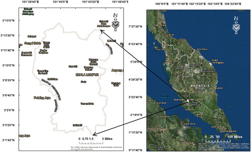
Kuala Lumpur urban area, alike to other metropolises in Southeast Asia and developing states, is facing air contamination problems related to heavy traffic. It is thus of importance to embark on research on predicting the air pollution levels and provide models which can be used to predict future levels in air quality.

3. Methodology

Along with basic data management and mapping tools, ArcGIS comprises analytical techniques that long been a foundation for GIS. Spatial statistic toolbox includes a set of methods for describing and modeling spatial information. As well as, they extend to assess the spatial pattern, processing, trends, distributions, and relationships. The methodology of the study has been applied in three steps; inverse distance weighted (IDW) geostatistical technique analysis, generation of regression models, and validation. The analysis of this study is based on two types of data; Malaysia climate database has been downloaded from NASA satellite data via RETScreen program and, daily historical data of AQI from the source of http://apims.doe.gov.my/ have been downloaded from https://air-quality.com/country/malaysia/44660bec?lang=en&standard=aqi%20us. Arc GIS version10.3 has been used for OLS model building and interpolation analysis, in addition to creating the outputs of the final maps included the legend and scale bar.

3.1. IDW

Inverse distance weighting (IDW) is the most communal process in GIS. IDW is a particular interpolator, hence the statistics values are well considered. The interpolation algorithm objective is to use measurements $z\left(s_i\right),$ $i=\mathrm{ }1,\mathrm{ }2,\dots ,\mathrm{ }n,$ set in points locations, to create an probability of the point value of the experimented property in the location $s_0$ when the observations are not existing. The weights given to elements are a function of the distance of the element from the estimate location. The weights are typically acquired through the inverse squared distance (signified by the exponent -2), and the estimate function of interpolation can be set as: (1) $$\widehat{z}\left(s_0\right)\frac{\sum _{i=1}^{n}z\left(s_i\right)d_{i0}^{-2}}{\sum _{i=1}^n{d}_{i0}^{-2}}$$(1) where $d_{i0}$ is the distance by which the s₀ and the $s_i$ are detached (Lloyd 2010). IDW was the best interpolation method in India air quality and had a smaller error than the kriging method in all pollutants (Jha et al. 2011). GIS offers a practical and significant working environment for integrating, analyzing, and visualizing these data together with new spatial data sources (Dobesch et al. 2013). The IDW was the best interpolation method to expect the air pollution conditions than Ordinary Kriging (OK) and Universal Kriging (UK) methods (Vorapracha et al. 2015). But, because of the minimum RMSE, Ordinary Kriging (OK) was the most accurate method for modeling AQI distribution (Saniei et al. 2016). Many studies have been carried out on air quality assessment using interpolation methods, the results of 71 methods showed that in most cases, the geostatistical processes is best than the deterministic techniques (Eslami and Ghasemi 2018).

AQI and meteorological records were statistically analyzed using GIS geospatial analysis techniques, based on IDW interpolation. For modeling meteorological patterns, climate database was obtained from three weather stations in Malaysia. The stations are Jerantut, Seremban, and Shah Alam. Temperature (T), Relative humidity (H), Wind speed (Ws), and Precipitation (P) data of the 3 months selected and analyzed using IDW from these stations, in addition to AQI data. IDW process was applied and the procedure was followed for every five parameters at all prediction locations. In this procedure, a worked sample of IDW is specified using three observations of each parameter, with the objective of predicting each parameter at another location in the study area.

3.2. OLS model

The standard method for fitting a provisional linear mean function to geostatistical data is OLS (Gelfand et al. 2010). OLS regression for k independent parameters is specified as: (2) $$z_i={\beta }_0+{\beta }_{1\mathrm{ }}{x}_{1i}+\dots +{\beta }_{k\mathrm{ }}{x}_{ki}+\epsilon$$(2)

Where $i$ denotes to a location, $x_{1i}\dots x_{ki}$ denote to the independent parameters at location $\mathrm{i},\mathrm{ }{\mathrm{\beta }}_0,\mathrm{ }{\mathrm{\beta }}_1,\mathrm{ }\dots ,{\mathrm{\beta }}_{\text{k }}$ are the parameters that will be predicted, and $\mathrm{\epsilon }$ denotes to the error term. In matrix form, this can be set as: (3) $$z=X\beta +\epsilon$$(3)

The variables of the model can be predicted via OLS thru solving: (4) $$\widehat{\beta }={(X}^T{X)}^{-1}{X^T}_Z$$(4) and the standard error is set as (Lloyd 2010): (5) $$\mathit{Var}\left(\widehat{\beta }\right)={\sigma }^2{(X}^T{X)}^{-1}$$(5)

Linear regressions are statistical techniques for modeling the linear relationships between variables to describe the relationship among a dependent variable and various independent variables in such a way that the behavior of the dependent one can be predicted from the independent variables if the relationship exists (Egbo and Bartholomew 2018). Linear regression is one of the more prevalent methods used, it is as well as common to use linear regression for its explanatory abilities rather than labels prediction. OLS is used in statistic to create a correlation among an attribute and a label in the presence of other features which are potentially correlated (Sheffet 2019).

GIS analysis can be used to investigate or quantify relations among variables. Modeling spatial relationships tool constructs spatial weight matrices or its modeling spatial relationship via regression analyses. The procedure for variable selection was AQI as a dependent variable and metrological parameters as independent variables to estimate AQI from metrological variables. Generating of the regression model, definitely, depends upon some aspects that essential to be taken into consideration. For instance, probability values for whole used factors in the equation must be less than 0.05. This value signifies the probability that none of the explanatory variables have an effect on the dependent variable. Also, the values of R² (R-Squared; Coefficient of Determination) and AdjR² (R-Squared adjusted for model complexity) should be high. All these aspects must be applied in order to obtain a high-quality model

3.3. Validation of OLS predictive algorithms

Information fitting is the method for fitting the model to information and analyzing how accurate the fit. Researchers practice the fitting process, involving mathematical calculations and nonparametric techniques permissible for modeling attained statistics (Shareef et al. 2014). Two types of validation have been applied, an accuracy value of model performance has been computed, given by the regression analysis model, and additionally testing model validation by using calculated AQI and comparing them with observed AQI data. Where 20 testing points used for testing the model and selected from IDW result different from the 45 trained points which were used for model building.

4. Results and discussion

4.1. The IDW analysis

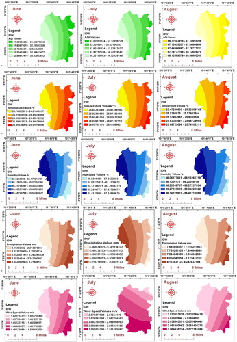
The analysis of IDW applied using the measured parameters values of the three stations to expect values for any site in the study area. The resultant IDW map included AQI, T, H, P, and Ws values classified as classes ranged by colors from low to high value. The estimated values are restricted to the range of the values used for interpolation. As IDW is a weighted distance average, hence, this average cannot be more than the higher value or lesser than the smaller value. Thus, it cannot create ridges or valleys if these limits have not previously been sampled. IDW of interpolation methods was used to define the cell values via a set of sites sample points. Comparing with other tools, the IDW is easier in applying in the program and no necessity to pre-modeling or subjective assumptions. Figure 2 represents IDW resultant maps of the period June to August 2018.

Figure 2. IDW resultant maps of the period June to August 2018. Source: Author

4.2. Air quality index OLS prediction models

By using the regression technique is easy to present equations to calculate AQI based on the category of independent variables used with a typical accurateness (97%). Summary of OLS results in June, July, and August 2018 are shown in Tables 1, 2, and 3 respectively.

Table 1. Summary of OLS results in June 2018.

Variable	Coefficient	StdError	t_Statistic	Probability	StdCoefficient
Intercept	−540.465431	207.5856928	−2.603577461	0.012884326	0
Temperature	−5.894326305	2.848119904	−2.069549915	0.044997269	−0.685345185
Humidity	7.975458349	1.674982207	4.76151825	2.51509E − 05	1.993337286
Wind speed	10.0685178	3.210469539	3.13615117	0.003206084	0.440862954
Precipitation	10.73357593	2.367889861	4.532970941	5.16269E − 05	1.305102285

Table 2. Summary of OLS results in July 2018.

Variable	Coefficient	StdError	t_Statistic	Probability	StdCoefficient
Intercept	−9.79689678	31.13020532	−0.314707105	0.754620902	0
Temperature	0.091779149	0.561712716	0.163391617	0.87103413	0.014818895
Humidity	0.192288445	0.231533815	0.830498325	0.411186016	0.074252353
Wind speed	3.53005047	0.741447404	4.76102614	2.51901E − 05	0.070997564
Precipitation	2.522535944	0.239144831	10.54815165	3.54945E − 13	0.930546222

Table 3. Summary of OLS results in August 2018.

Variable	Coefficient	StdError	t_Statistic	Probability	StdCoefficient
Intercept	−430.2939518	200.9159091	−2.14166192	0.038365026	0
Temperature	−1.393425327	0.631913806	−2.205087645	0.033260506	−0.226165684
Humidity	5.826824717	2.159007789	2.698843769	0.010144625	1.159345533
Wind speed	18.12528468	2.562350227	7.073695271	1.42851E − 08	0.718066005
Precipitation	−0.741358189	1.254253379	−0.591075298	0.557794921	−0.254550825

Once regression and modeling analysis has been completed, three analytical models to observe AQI have been prepared. As well as we tested the modeling and correlation among dependent and independent parameters based on the mentioned conditions.

The obtained three modeling equations that have been set for the records for the period of June to August indicated in Equations (6(6) $${\mathrm{AQI}}_{\mathrm{calculated}}=-540.465-5.899\mathrm{ }T+7.975\mathrm{ }H+10.068\mathrm{ }Ws+10.733P$$(6) , 7, and 8) respectively. (6) $${\mathrm{AQI}}_{\mathrm{calculated}}=-540.465-5.899\mathrm{ }T+7.975\mathrm{ }H+10.068\mathrm{ }Ws+10.733P$$(6) (7) $${\mathrm{AQI}}_{\mathrm{calculated}}=-9.796+3.530\mathrm{ }Ws+2.522\mathrm{ }P$$(7) (8) $${\mathrm{AQI}}_{\mathrm{calculated}}=-430.293-1.393\mathrm{ }T+5.826\mathrm{ }H+18.125\mathrm{ }Ws$$(8)

Where, AQI represents the Air Quality Index value, T (°C) represents the temperature, H (%) represents the relative humidity, $Ws$ (m/sec) represents the wind speed, and P (mm) represents precipitation. Parameters were used; AQI as a dependent variable, H, T, Ws, and P as independent variables. Based on the chosen data from IDW results and NASA satellite data, which have been collected via the RETScreen program, the OLS model equations were introduced to estimate the AQI values at all recorded points. Depending on the basic formula of multiple linear regression equation, the statistical analysis for model constructing was conducted through three runs of variable selection. The first case, the OLS was employed to analyze the relationship between each independent variable and the dependent variable AQI. The employed data have been collected in June. The introduced equation included all parameters used in the modeling is represented in Equation (6)(6) $${\mathrm{AQI}}_{\mathrm{calculated}}=-540.465-5.899\mathrm{ }T+7.975\mathrm{ }H+10.068\mathrm{ }Ws+10.733P$$(6) .

The second case, the OLS regression model was used to analyze the relationship between the independent variables and the dependent variable AQI. The employed data have been collected in July. The introduced equation included precipitation and wind speed used in the modeling. It is necessary to identify the potential dependencies amongst the predictors for model specification. Here the temperature has no impact in July. The correlation matrix limits the strength of linear relationships. Most of the tested parameters of a high level of collinearity with others, except in temperature and humidity in this case only. The probability value of temperature is 0.87 as shown in Table 2, which is more than 0.05 so, it has been excluded from the equation. The studies specify the correlation to be more than 0.70 as a good correlation. Nevertheless, in this case of analysis, the aim was to attain the lowest relationship among studied variables to study of their impact. Therefore, we depended on two parameters that can be used to create the regression model represented in Equation (7)(7) $${\mathrm{AQI}}_{\mathrm{calculated}}=-9.796+3.530\mathrm{ }Ws+2.522\mathrm{ }P$$(7) .

The third case employed data collected during August to predict AQI values. The model that we have obtained represented in Equation (8)(8) $${\mathrm{AQI}}_{\mathrm{calculated}}=-430.293-1.393\mathrm{ }T+5.826\mathrm{ }H+18.125\mathrm{ }Ws$$(8) included temperature, humidity and wind speed variables. Also, because of no correlation, we excluded the precipitation variable from the equation and model constructing.

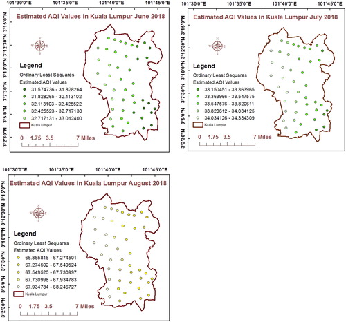
In fact, these equations do not produce the absolute values of the predicted variable but denote to the closed or near approximated to the real value. The physical significance of coefficients in the equations represents the best optimization, which refers to the close value of real value that can be estimated. Two types of data were used for model equation construction. For correlation and model construction NASA satellite data were utilized. For the absence of AQI data of NASA, we used daily historical data of AQI obtained from The Global Air Quality Service Provider in order to validate and test correlation. All estimated mathematical equations have accuracy correspondent to R² as well as probability value obtained from the regression analysis of the model. In completely estimated models equations, we utilized the forward computations in order to achieve the extra high R² adjusted. The obtained models showed a high correlation between the AQI and the independent variables. Where Ws was the most important independent variable more contribute the estimation then P was the next contributor followed by the other variables. The strong and medium winds generate turbulent environments and local disturbances in the environs which results in the hazy environment and dust storm which cause increasing of the particles sizes (Mamta and Bassin 2010). Effects of meteorological parameters may perhaps be the alternatives factors in the explanation of the differences of the observed R values, because of their non-negligible impacts (Guo et al. 2017). In Figure 3, the regression resultant map of AQI estimation of each predictive model of the period June to August 2018 has been represented.

Figure 3. The regression resultant map of AQI estimation of each predictive model of the period June to August 2018. Source: Author

4.3. Validating of OLS predictive algorithms

Two types of validation have been used in order to examine the power of the achieved models. The confidence bounds models analysis were applied to determine the estimated algorithm's accuracy. Validation of estimated algorithms applied by both trained and tested points selected randomly. The result showed that all selected points that used have well fit besides all stations fall in the confidence range.

4.3.1. OLS model validation

As shown in Figure 4, using 45 training points the validation has been practiced. This validation uses the polynomial linear fitting to estimate AQI values by OLS model and compare them with trained (observed) AQI.

Figure 4. OLS model validation. Source: Author

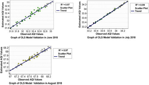
The validation applied for all 3 months. The results showed the whole records are in the confidence boundary with R² up to 0.97 in June and August, and 0.99 in July. Here the observed AQI values refer to the entered values in the model building and the estimated AQI values refer to the predicted values by regression analysis and model building. The goal of applying the predicted algorithms by trained points is to achieve the typical accuracy and to test the amount of equivalent at the point position.

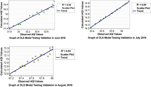
4.3.2. OLS model testing validation

As shown in Figure 5, using 20 testing points, the validation and degree of confidence have been practiced again. Polynomial linear fitting is the base of this validation in this study in order to obtain AQI values by estimation models then compare them with tested (observed) AQI. Additionally to examine the performance of the model using different testing points. The result showed that all calculated parameters demonstrated a good agreement with observed parameters with R² equal to (0.96, 0.99, and 0.93), respectively. Here the calculated AQI values refer to the calculated points by regression equations using testing parameters.

Figure 5. OLS model testing validation. Source: Author

5. Conclusion

In this research, prospective application for analyzing and modeling the AQI has been demonstrated by OLS based GIS technique and IDW geostatistical analysis. The aim of this approach was to present an AQI analytical estimation model. Three equations have been introduced to predict AQI from metrological parameters (temperature, humidity, wind speed, and precipitation) for the period from June to August 2018. In this study, we utilized the data obtained from the IDW analysis in the production of the three predicting AQI models. Moreover, high accuracies have been obtained given by regression analysis and model testing analysis, where maximum accuracy value was 99% in July indicating the parameter wind speed more contribute AQI predicting then precipitation. Furthermore, significant applied and methodological outputs presented using the IDW with OLS regression. It yields predictions of daily AQI levels with high predictive accuracy. These models offer detailed statistics and accurate maps of air pollutant levels distribution in addition to predicting air quality levels.

Acknowledgements

The authors would like to thank Dr. Muntadar A. Shareef for his assistance with the statistical programming. The data of this study were obtained from the NASA satellite via RETScreen program funded through the CanmetENERGY Research Center of the Natural Resources Canada’s NRCan. We are also thankful to the RIKEN Centre for Advanced Intelligence Project (AIP), Tokyo, Japan for the funding support.

Disclosure statement

No potential conflict of interest was reported by the authors.

Additional information

Funding

The authors would like to thank the RIKEN Centre for Advanced Intelligence Project (AIP), Japan for the APC funding.

References

- Ahmad A, Hashim M, Hashim MN, Ayof MN, Budi AS. 2009. The use of remote sensing and GIS to estimate Air Quality Index (AQI) Over Peninsular Malaysia. GIS development. https://www.geospatialworld.net/linkout/154551.
- Ajaj QM, Pradhan B, Noori AM, Jebur MN. 2017. Spatial monitoring of desertification extent in western Iraq using Landsat images and GIS. Land Degrad Develop. 28(8):2418–2431. doi:10.1002/ldr.2775.
- Anjum SS, Noor RM, Aghamohammadi N, Ahmedy I, Kiah MLM, Hussin N, Anisi MH, Qureshi MA. 2019. Modeling traffic congestion based on air quality for greener environment: an empirical study. IEEE Access. 7:57100–57119. doi:10.1109/ACCESS.2019.2914672.
- Cheong Y, Burkart K, Leitão P, Lakes T. 2013. Assessing weather effects on dengue disease in Malaysia. Int J Environ Res Public Health. 10(12):6319–6334. doi:10.3390/ijerph10126319.
- Corwin DL, Wagenet RJ. 1996. Applications of GIS to the modeling of nonpoint source pollutants in the vadose zone: a conference overview. J Environ Qual. 25(3):403–411. doi:10.2134/jeq1996.00472425002500030004x.
- Dadhich AP, Goyal R, Dadhich PN. 2018. Assessment of spatio-temporal variations in air quality of Jaipur city, Rajasthan, India. Egypt J Remote Sens Space Sci. 21(2):173–181. doi:10.1016/j.ejrs.2017.04.002.
- Dobesch H, Dumolard P, Dyras I. 2013. Spatial interpolation for climate data: the use of GIS in climatology and meteorology. 2nd ed. New York: Wiley. https://books.google.iq/books?isbn=1118614992.
- Egbo MN, Bartholomew DC. 2018. Forecasting students’ enrollment using neural networks and ordinary least squares regression models. J Adv Stat. 3(4):45–57. doi:10.22606/jas.2018.34001.
- Eslami A, Ghasemi SM. 2018. Determination of the best interpolation method in estimating the concentration of environmental air pollutants in Tehran city in 2015. J Air Pollut Health. 3(4):187–198. doi:10.18502/japh.v3i4.402.
- Gattrell A, Loytonen M, editors. 1998. GIS and Health. 1st ed. Vol. 6. Boston (MA): Houghton Mifflin Harcourt.
- Gelfand AE, Diggle P, Guttorp P, Fuentes M. 2010. Handbook of spatial statistics. 1st ed. Boca Raton (FL): CRC Press. doi:10.1201/9781420072884.
- Guo J, Xia F, Zhang Y, Liu H, Li J, Lou M, He J, Yan Y, Wang F, Min M, et al. 2017. Impact of diurnal variability and meteorological factors on the PM2. 5-AOD relationship: implications for PM2. 5 remote sensing. Environ Pollut. 221:94–104. doi:10.1016/j.envpol.2016.11.043.
- Hashim NI, Yusof NHS, Anuar ANA, Sulaiman FC. 2019. The restorative environment offered by Pocket Park at Laman Standard Chartered Kuala Lumpur. J Hotel Bus Manage. 8(194):2169–0286. doi:10.4172/2169-0286.1000194.
- He Q, Huang B. 2018. Satellite-based mapping of daily high-resolution ground PM2. 5 in China via space-time regression modeling. Remote Sens Environ. 206:72–83. doi:10.1016/j.rse.2017.12.018.
- Jha DK, Sabesan M, Das A, Vinithkumar NV, Kirubagaran R. 2011. Evaluation of Interpolation Technique for Air Quality Parameters in Port Blair, India. Univ J Environ Res Technol. 1(3):301–310. http://www.environmentaljournal.org/1-3/ujert-1-3-10.pdf.
- Jumaah HJ, Mansor S, Pradhan B, Adam SN. 2018. UAV-Based PM2. 5 Monitoring for small-scale urban areas. Int J Geoinf 14(4):61–69. https://www.researchgate.net/publication/333378629_UAVbased_PM25_monitoring_for small-scale_urban_areas.
- Liu CM. 2002. Effect of PM2. 5 on AQI in Taiwan. Environ Model Softw. 17(1):29–37. doi:10.1016/S1364-8152(01)00050-0.
- Lloyd CD. 2010. Local models for spatial analysis. 2nd ed. Boca Raton (FL): CRC Press.
- Lü G, Batty M, Strobl J, Lin H, Zhu AX, Chen M. 2019. Reflections and speculations on the progress in Geographic Information Systems (GIS): a geographic perspective. Int J Geogr Inf Sci. 33(2):346–367. doi:10.1080/13658816.2018.1533136.
- MacKerron G, Mourato S. 2009. Life satisfaction and air quality in London. Ecol Econ. 68(5):1441–1453. doi:10.1016/j.ecolecon.2008.10.004.
- Mamta P, Bassin JK. 2010. Analysis of ambient air quality using air quality index–a case study. Int J Adv Eng Technol. 1(2):106–114.
- McLafferty SL. 2003. GIS and health care. Annu Rev Public Health. 24(1):25–42. doi:10.1146/annurev.publhealth.24.012902.141012.
- Murayama Y, Thapa RB. 2011. Spatial analysis and modeling in geographical transformation process. 1st ed. Vol. 100. New York: The GeoJournal Library. doi:10.1007/978-94-007-0671-2.
- Nyerges TL, Jankowski P. 2009. Regional and Urban GIS: a decision support approach. 1st ed. New York: Guilford Press.
- Pisoni E, Christidis P, Thunis P, Trombetti M. 2019. Evaluating the impact of “Sustainable Urban Mobility Plans” on urban background air quality. J Environ Manag. 231:249–255. doi:10.1016/j.jenvman.2018.10.039.
- Poursafa P, Mansourian M, Motlagh ME, Ardalan G, Kelishadi R. 2014. Is air quality index associated with cardiometabolic risk factors in adolescents? The CASPIAN-III study. Environ Res. 134:105–109. doi:10.1016/j.envres.2014.07.010.
- Saniei R, Zangiabadi A, Sharifikia M, Ghavidel Y. 2016. Air quality classification and its temporal trend in Tehran, Iran, 2002-2012. Geospat Health. 11(2):213–220. doi:10.4081/gh.2016.442.
- Shareef MA, Toumi A, Khenchaf A. 2014. Prediction of water quality parameters from SAR images by using multivariate and texture analysis models. In SAR Image Analysis, Modeling, and Techniques XIV; October; Vol. 9243, p. 924319. Amsterdam, Netherlands : SPIE Remote Sensing. doi:10.1117/12.2067262.
- Sharma R, Balasubramanian R. 2019. Assessment and mitigation of indoor human exposure to fine particulate matter (PM2. 5) of outdoor origin in naturally ventilated residential apartments: A case study. Atmos Environ. 212:163. doi:10.1088/1748-9326/aa86dd.
- Sheffet O. 2019. Differentially private ordinary least squares. J Privacy Confid. 9(1): 1-43. doi:10.29012/jpc.654.
- Somvanshi SS, Vashisht A, Chandra U, Kaushik G. 2019. Delhi air pollution modeling using remote sensing technique. In: Hussain C, editor. Handbook of environmental materials management. Cham: Springer; p. 1–27. doi:10.1007/978-3-319-58538-3_174-1.
- Sreetheran M. 2017. Exploring the urban park use, preference and behaviours among the residents of Kuala Lumpur, Malaysia. Urban For Urban Green. 25:85–93. doi:10.1016/j.ufug.2017.05.003.
- Tian B. 2016. GIS technology applications in environmental and earth sciences. 1st ed. Boca Raton (FL): CRC Press. doi:10.1201/9781315366975.
- Tian Y, Yao X, Chen L. 2019. Analysis of spatial and seasonal distributions of air pollutants by incorporating urban morphological characteristics. Comput Environ Urban Syst. 75:35–48. doi:10.1016/j.compenvurbsys.2019.01.003.
- Twomey PJ, Kroll MH. 2008. How to use linear regression and correlation in quantitative method comparison studies. Int J Clin Pract. 62(4):529–538. doi:10.1111/j.1742-1241.2008.01709.x.
- Vorapracha P, Phonprasert P, Khanaruksombat S, Pijarn N. 2015. A comparison of spatial interpolation methods for predicting concentrations of Particle Pollution (PM10). Int J Chem Environ Biol Sci. 3(4):302–306.
- Wu CF, Larson TV, Wu SY, Williamson J, Westberg HH, Liu LJS. 2007. Source apportionment of PM2. 5 and selected hazardous air pollutants in Seattle. Sci Total Environ. 386(1–3):42–52. doi:10.1016/j.scitotenv.2007.07.042.
- Yang Y, Zheng Z, Bian K, Song L, Han Z. 2018. Real-time profiling of fine-grained air quality index distribution using UAV sensing. IEEE Internet Things J. 5(1):186–198. doi:10.1109/JIOT.2017.2777820.
- Zain SNM, Behnke JM, Lewis JW. 2012. Helminth communities from two urban rat populations in Kuala Lumpur, Malaysia. Parasit Vectors. 5(1):47. doi:10.1186/1756-3305-5-47.
- Zheng Y, Liu F, Hsieh HP. 2013. U-Air: when urban air quality inference meets big data. In Proceedings of the 19th ACM SIGKDD International Conference on Knowledge Discovery and Data Mining; August. p. 1436–1444. ACM.Chicago, Illinois, USA. doi:10.1145/2487575.2488188.