Application of NRCS-CN method for estimation of watershed runoff and disaster risk

Abstract

The NRCS-CN method is widely applied in the estimation of precipitation runoff. It primarily relies on soil mapping and land use data as input parameters, although land use data is not frequently updated. This study replaced such data with land cover classes based on satellite images, and found this approach favorable to investigate how land use affect runoff. The study further determined the relationship between typhoon events (between 2005 and 2009) and natural hazards using Chenyoulan watershed located in central Taiwan. to The Nash–Sutcliffe model efficiency coefficient was used to assess the accuracy of the NRCS-CN method, which revealed an efficiency coefficient as high as 90.8%. Numerous studies have applied the mean curve number of the whole watershed as the unit of analysis, resulting in poor fit between estimated and observed values. Therefore, this study employed the estimated values of the grids where the monitoring stations were located to form a relationship curve with observed values. This corrected the runoff values and improved the estimation of runoff in the watershed. Furthermore, the model can be applied to simulate runoff depths of grids, and estimate flooding risk, providing a reference for watershed disaster management.

Keywords:

• Curve number
• typhoon event
• runoff
• disaster risk

1. Introduction

Studies have demonstrated extensive application of remote sensing technologies in research areas such as land-use survey, environmental analysis, and slope disaster prevention (Ayanlade and Howard 2017; Cheţan et al. 2018; Swinbourne et al. 2018). In addition to reducing the surveying time in comparison with that required in conventional survey methods, remote sensing technology can reach regions that are inaccessible or dangerous to humans. Therefore, such technology can be adopted for land-use surveys in a largescale drainage basin having complex terrain. The use of predictive modeling on the relationship between watershed precipitation and runoff is instrumental in the management of flood hazards. Numerous studies on flood estimation have been published, most of which aim to more precisely discern the relationship between precipitation and runoff (Guru and Jha 2015; Li and Zhang 2017).

The frequency of floods is related to the characteristics of a watershed, including changes in land use induced by urbanization, which can reduce ground infiltration and increase surface runoff. For this reason, the development of a suitable model capable of using land use data to accurately predict the relationship between watershed precipitation and runoff should be prioritized. Understanding the characteristics of precipitation is crucial in controlling flood hazards, because surface runoff occurs when the intensity of precipitation surpasses the infiltration capacity. Moreover, land development intensity and soil characteristics affect the land’s capacity to retain water. The association between precipitation and runoff is complicated, dynamic, and nonlinear. Research on this subject is often difficult task because it entails long-term monitoring of a watershed, which is often impeded by the lack of monitoring stations or data. This has given rise to numerous predictive models for precipitation-runoff simulation, including the Tank model, HBV model, MIKE 11/NAM model, and NRCS-CN) model. Of these models, the NRCS-CN model is the most widely used for the estimation of runoff in watersheds where monitoring stations are lacking (Fan et al. 2013).

The NRCS-CN model was developed in 1972 by the US Soil Conservation Service (SCS), which was the predecessor of the Natural Resources Conservation Service (NRCS). The model makes extensive use of runoff curve number, which is also referred to as curve number (CN), to estimate surface runoff in a watershed. In this model, empirical data are used to simulate the relationship between stormwater and local hydraulic changes, and this approach enables the prediction of storm runoff from rainfall depth. Lately, the CN has been increasingly applied in fields pertaining to engineering, hydrology, and water resource management and has returned favorable results (Huang et al. 2006; Jung et al. 2012; Ozdemir and Elbaşı 2015).

Floods have become a global hazard and Taiwan is not immune. Her climate and terrain often induce instantaneous heavy rainfall and prolonged rainfall, which often lead to disastrous floods and subsequent loss of life and property (Yang et al. 2015). Located in the subtropics, Taiwan enjoys abundant rainfall associated with the monsoon rain in May and June, which is also known as plum rain. Taiwan’s mean annual rainfall is approximately 2500 mm, which is 2.6 times the world average (Tung and Pai 2015). Moreover, Taiwan is prone to typhoons between July and October, because it is in the path of most typhoons formed in the northwest Pacific. Typhoons are among the most dangerous and destructive natural hazards Taiwan is subjected to. For example, in 2009, Typhoon Morakot inflicted extremely heavy loss of life and property, with official statistics indicating that the associated floods alone were responsible for 681 deaths, with 18 missing (Lee et al. 2013). The watershed of the Chenyoulan River was among the most heavily hit; the raging torrent scoured riverbanks and blocked road networks, causing numerous waterfront properties to be swept away.

This study selected the Chenyoulan watershed for big data analysis, in which actual monitoring data were used to verify inferred runoff values in typhoon events. Additionally, environmental indicators were applied in risk assessment conceptual modeling, which analyzed hazard and vulnerability levels to establish a risk model. This model, which is capable of predicting areas that are vulnerable to sudden rise of water level, can be instrumental in hazard management.

2. Materials and methods

2.1. Study area

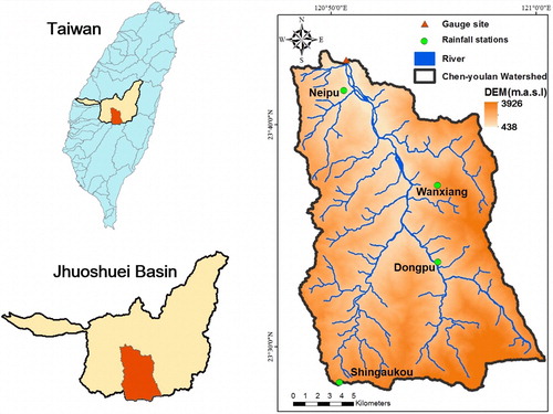
The Chenyoulan watershed is located in central Taiwan at approximately 23°20'−23°35'N, 120°47'−121°00'E (Figure 1). A tributary of the Jhuoshuei River, the Chenyoulan is roughly 42 km in length. Its watershed encompasses an area approximately 448 km² in size, where the annual average temperature is 19 − 23 °C, and receives an annual rainfall of 1600 − 2600 mm. This drainage basin forms a narrow and elongated fault-line valley that converges water from the north face of Yushan (Jade Mountain), the east face of the Alishan range, and the west face of the Jyunda range. As such, the main stream runs from south to north, and the tributaries flow into the main stream from east and west slopes (Lin et al. 2004). The main stream forms a longitudinal valley that is relatively straight, with the left bank made up of Miocene sedimentary rock formations and the right bank made up of Paleogene slate formations (Lee 1996).

Figure 1. Watershed with locations of rainfall stations and gauge sites. Source: Author

2.2. Study materials

The study materials are listed in Table 1. The land cover types were based on satellite image records from the United States Geological Survey, which were further verified by aerial photographs. Soil map was based on soil hydrology module of the Soil and Water Conservation Bureau, which, together with the land cover data, were used to infer the spatial distribution of CN values. Rainfall and runoff data, which were used to verify the long-term runoff predictions, were taken from the monitoring data of the Water Resources Agency. Additionally, a digital elevation model (DEM) with 5 × 5 grids was used to determine the administrative divisions of the watershed and for the extraction of topographic wetness indices (TWIs).

Table 1. Study materials.

Map/information	Year	Resolution	Source	Application
Satellite imagery (Landsat)	1990 ∼ 2010	30m*30m	U. S. geological survey	Land cover types extraction to estimate CN
Aerial photography	2010	1/5000	Google Earth	Land cover verification
DEM	2004	5m*5m	Department of land administration	Terrain analysis
Soil	2005	1/5000	Soil and water conservation bureau	To calculate CN
Rainfall	2005 ∼ 2009	Daily data	Water resources agency	Estimation of direct runoff
Runoff	2005 ∼ 2009	Daily data	Water resources agency	Model verification

2.3. Methods

The research method consisted of Seven parts: (a) Satellite image classification, (b) Accuracy assessment of Land use (Land cover), (c) NRCS-CN method, (d) Hydrological data collection, (e) Performance and efficiency, (f) Risk analysis, and (g) Buffer zone. Details of the research method are described as follows:

2.3.1. Satellite image classification

Radiant energy is absorbed by plants during photosynthesis, whereas near-infrared light either passes through them or is reflected. These characteristics have been extensively used by researchers to determine the status of groundcover. For this purpose, normalized difference vegetation index (NDVI) has been defined as the difference in the near-infrared and red spectral reflectance measurements, divided by the sum of their spectral reflectance measurements. As such, the value of NDVI ranges from −1 to 1, with a higher value denoting greater plant growth. The formula is as follows: (1) $$\text{NDVI}\hspace{0.17em}=\hspace{0.17em}\left(\text{NIR}\hspace{0.17em}-\hspace{0.17em}\mathrm{R}\right)/\left(\text{NIR}\hspace{0.17em}+\hspace{0.17em}\mathrm{R}\right)$$(1) where NIR and R denote the reflectance of near-infrared and visible red bands, respectively.

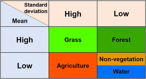
In Taiwan, summer is the rainy season and winter the dry season. Therefore, satellite images of these two seasons were analyzed by the mean and standard deviation values of NDVI. K-mean clustering was subsequently performed to divide the mean and standard deviation values into a ‘high’ group and a ‘low’ group. A high mean value denoted thriving growth of groundcover during both seasons, whereas a low mean value denoted sparse groundcover growth between the two seasons. In addition, a high standard deviation value denoted considerable groundcover changes between the seasons, whereas a low standard deviation value denoted limited groundcover changes. Furthermore, the products of the mean and standard deviation values yielded four more classifications, namely agriculture, grass, forest, and non-vegetation. In addition, a supervised classification method was used to extract waterlogged areas from the non-vegetation class (Figure 2).

Figure 2. Using statistical methods to sort land use on the basis of satellite images. Source: Author

2.3.2. Accuracy assessment of land use (land cover)

After classification, the satellite images were compared with aerial photographs (pixel comparison) to determine whether the classification had sufficient accuracy. Specifically, this was achieved by using an error matrix to analyze the overall accuracy (OA) and Kappa coefficient, based on which classification accuracy was judged (Fang 2003; Lin 2012). OA was acquired by dividing the total number of accurately classified samples with the total number of samples. OA is an objective approach because it takes the relative weight of each class into consideration. The formula is as follows: (2) $$OA\mathrm{ }=\mathrm{ }\left(\frac{{\sum }_{i=1}^n{X}_{ii}}{{\sum }_{i=1}^n{\sum }_{j=1}^n{X}_{ij}}\right)\mathrm{ }\times 100\mathrm{\%}$$(2) where X_ii denotes the number of samples with accurately classified groundcover types, X_ij denotes the element at the i-th row and j-th column of the error matrix, and n denotes the number of classes.

Additionally, the Kappa coefficient was used to assess interpretation results and results of random classification. Its formula is as follows: (3) $$\text{Kappa coefficient}=\frac{N{\sum }_{i=1}^n{X}_{ii}-{\sum }_{i=1}^n\left(X_{i+}\mathrm{*}{X}_{+i}\right)}{N^2-{\sum }_{i=1}^n\left(X_{i+}\mathrm{*}{X}_{+i}\right)}$$(3) where N denotes the total number of sample points, X_ii denotes the number of sample points on the diagonals of the classification matrix, X_i+ is the sample number of each column in the classification matrix, X_+i is the sample number of each row in the classification matrix, and n denotes the number of rows in the classification matrix. The Kappa coefficient can be derived from the calculations of an error matrix, making it widely applied in assessing the interpretation accuracy of remote sensing images. The Kappa coefficient ranges between 0 and 1, with a higher value denoting a higher accuracy. Typically, a value above 0.7 is considered to indicate excellent classification results, whereas a value below 0.4 indicates poor classification (Congalton 1991; Janssen and Vanderwel 1994). Employing satellite images to analyze land use can reduce the human and material resources required in land-use surveys and shorten the surveying time. Satellite images revealed that the types of land used consisted of farmlands, grasslands, forests, non-vegetated areas, and water areas.

Subsequently, aerial photographs captured in 2010 were used to assess the accuracy of the land cover analysis, and the results indicated an OA of 92% and Kappa coefficient of 0.71 (Table 2). A Kappa coefficient greater than 0.70 indicated that the sorting of land-use type achieved favorable results, which a satellite image analysis revealed to be the case for the Chenyoulan drainage basin.

Table 2. Results of accuracy assessment.

Observed Estimated	Non-vegetation	Forest	Agricultural	Grass	Water	Total
Non-vegetation	33	0	0	0	0	33
Forest	8	315	4	6	1	334
Agricultural	1	3	5	0	0	9
Grass	0	12	0	7	0	19
Water	0	0	0	0	5	5
Total	42	330	9	13	6	400

Overall accuracy = 92%, Kappa = 0.71.

2.3.3. NRCS-CN method

The NRCS-CN method is a simple method that is widely applied in engineering, hydrology, and watershed management. It is suitable for scenarios where monitoring data are lacking, because it draws input parameters from land use, land cover, and soil information (primarily satellite images and soil maps), which can be easily acquired. Regarding land-use type sorting in this study, satellite statistics were adopted to analyze the NDVI value of each grid. The seasonal differences in the conditions of vegetation coverage, the means and standard deviations obtained using statistical methods were employed to sort land parcels according to their use (Figure 2). The CN values of individual grids were determined by looking up the national engineering handbook using land-use sorting results and parameters of hydrologic soil groups (HSGs). In this study, the NRCS-CN method was used to predict the relationship between precipitation and runoff (NRCS 1972). The formula is as follows: (4) $$Q=\hspace{0.17em}0,P<\hspace{0.17em}0.2S$$(4) (5) $$Q=\hspace{0.17em}{\left(P-\hspace{0.17em}0.2S\right)}^2/\left(P+\hspace{0.17em}0.8S\right),P>\hspace{0.17em}0.2S$$(5) where Q denotes direct runoff depth (mm), P denotes storm rainfall depth (mm), and S denotes potential maximum retention (mm). The relationship between S and CN can be expressed as follows: (6) $$S=\hspace{0.17em}\left(25400/\text{CN}\right)\hspace{0.17em}–\hspace{0.17em}254$$(6)

The mean CN values for watersheds were computed using the following formula: (7) $${CN}_{av}\mathrm{ }=\sum A_i\mathrm{*}{CN}_i/\sum A_i$$(7) where CN_av denotes the mean CN value of the watershed, A_i denotes the area (m²) of a grid, and CN_i denotes the CN value of the grid.

2.3.4. Hydrological data collection

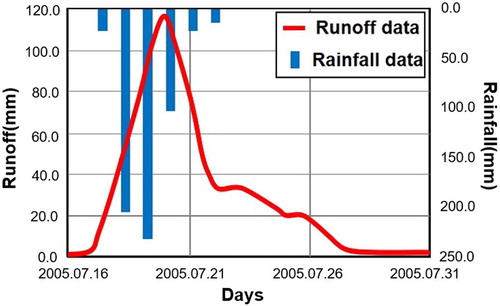
This study adopted the CN value method, using the measured precipitation to simulate runoff in the drainage basin and the measured runoff to assess the modeling accuracy. To successfully complete the model analysis, the authors obtained data of measured precipitation and runoff from the Water Resources Agency, Ministry of Economic Affairs. The four precipitation stations in the Chenyoulan drainage basin (Figure 1), namely the Neimaopu, Wanxiang, Dongpu, and Shingaukou Stations, are located upstream, midstream, and downstream from the Chenyoulan River. To calculate the average precipitation of the drainage basin, Thiessen’s polygon method was used to analyze the weights of individual precipitation stations. The average precipitation could then be calculated from the product of the weight and precipitation level of each station. The runoff produced by individual precipitation events could be monitored from the Neimaopu flow-observation station downstream from the Chenyoulan drainage basin. The runoff after Typhoon events was monitored in this study. Base flow was separated to eliminate its interference through the straight-line method, to determine the relationship between precipitation and runoff. Using the 2005 Typhoon Haitang as an example, a relation chart of rainfall and runoff was plotted based on relevant data (Figure 3). The figure displays the corresponding runoff of the rainfall at different time periods.

Figure 3. Rainfall and runoff for HAITANG typhoon event. Source: Author

2.3.5. Performance and efficiency

The accuracy of the simulation data was compared with the monitored data of a long-term runoff event using the Nash–Sutcliffe model efficiency coefficient (NSE), expressed as follows (Nash and Sutcliffe 1970): (8) $$\mathrm{NSE}\mathrm{ }=\mathrm{ }1-\mathrm{ }\frac{\sum (Q_{\mathit{obs}}-Q_{\mathit{comp}}{)}^2}{\sum (Q_{\mathit{obs}}-Q_{av})}\times \mathrm{ }100$$(8) where Q_obs denotes observed runoff, Q_comp denotes modeled runoff, and Q_av denotes mean observed runoff.

2.3.6. Risk analysis

The risk analysis performed in this study adopted the risk calculation model proposed by the United Nations Disaster Relief Organization (1979), which considered risk as a combination of hazard (the intensity and incidence of a hazard) and vulnerability (the capacity to withstand a hazard), expressed as the following formula (Chen et al. 2009): (9) $$\text{Risk}＝\text{hazard}\hspace{0.17em}\times \hspace{0.17em}\text{vulnerability}$$(9)

The construction of a drainage-basin flood risk assessment model requires a substantial amount of human and material resources. By comparison, the extraction of hazard and vulnerability values from big data not only yields accurate analysis results but also requires a shorter time for model construction and lower expenditure on research and development. The hazard and vulnerability data adopted in the model analysis were the accumulative event rainfall and the DEM of the drainage basin.

In this study, the hazard of a region with flood risk was determined by employing the rainfall data of Typhoon Morakot and the SCS runoff curves using the CN values for normalized excessive rainfall values. The data can be estimated by substituting the cumulative rainfall of Typhoon Morakot into Equation (5)(5) $$Q=\hspace{0.17em}{\left(P-\hspace{0.17em}0.2S\right)}^2/\left(P+\hspace{0.17em}0.8S\right),P>\hspace{0.17em}0.2S$$(5) . Excessive rainfall represents the influence of a rainfall event on flood probability and intensity. Higher values indicate more substantial effects of a disaster to the drainage basin.

The vulnerability was determined using normalized TWIs obtained through a terrain analysis. The TWI, which is widely used in topographic and hydrologic studies, can be obtained using the upslope area and slope of the targeted region (Sörensen et al. 2006). The formula is as follows: (10) $$\mathit{TWI}=\hspace{0.17em}\hspace{0.17em}\text{ln}\hspace{0.17em}\hspace{0.17em}\left(As/\hspace{0.17em}\text{tan}\hspace{0.17em}\beta \right)$$(10) where As denotes the area of the targeted drainage basin, particularly the upslope area draining through a grid; and β denotes the slope (radian) of the grid. The terrain humidity index reflects the cumulative capacity of runoff. If a grid is located downstream from the drainage basin and is part of the low-lying land, then the runoff in that grid tends to accumulate; therefore, topographically, the grid is susceptible to flooding.

2.3.7. Buffer zone

To mitigate the damage inflicted on riverbanks scoured by flooding, the concept of a riparian buffer zone was introduced (Lin et al. 2002). In this study, hydrographic, slope aspect, and elevation data were used to determine the elevation differences between the river banks and centerline of river channels. In regions where the elevation difference was found to be smaller than the flood level plus the depth of bottom scouring, a buffer zone should be created and the region should not be developed.

3. Results and discussions

3.1. Land use (land cover) and CN values

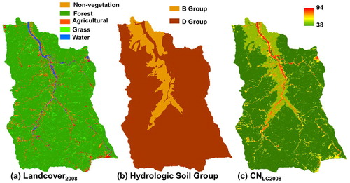
In this study, the land use of the drainage basin was determined by using satellite images. Aerial photographs were then used to evaluate the accuracy of land-use sorting (Figure 4). The results indicated that satellite images can be effective for land-use sorting. Figure 5(a) presents the 2008 land-use sorting results. Land parcels were sorted into five categories: non-vegetated areas, forests, farmlands, grasslands and water areas. Specifically, non-vegetated areas comprise construction and bare-land locations. Forests are locations that feature stable vegetation, minimal vegetation variance, and a high density of plant growth. Farmlands are primarily crop-planting locations. Grasslands are subject to seasonal variations and have relatively thriving vegetation during the rainy season. Water areas primarily consist of river channels and pools. The spatial distribution of soil in the drainage basin were obtained from the Soil and Water Conservation Bureau. The results of this inquiry indicated that the upstream area of the drainage basin is primarily composed of stone soil, whereas the downstream area primarily consists of colluvial soil. This information can serve as a reference for analyzing the spatial distribution of the HSGs in the investigated area. Figure 5(b) presents the HSG results; Group B consisted of areas located in proximity to river channels, and the remaining locations in the drainage basin were classified as Group D. Typically, under HSG classification, the infiltration rate of Group B was higher than that of Group D. Accordingly, when both groups were subject to the same type of land use, Group B generally demonstrated less runoff than Group D. The runoff of the drainage basin could be simulated using the CN value method, where land use, land-cover type, and HSG were the primary input parameters. With the global information system, drainage basin parameters can be used to estimate the spatial distribution of CN values in the drainage basin. Figure 5(c) depicts the spatial distribution of the CN values of each grid in the drainage basin, which indicated that relatively high CN values were mainly distributed along the river channels and nearby locations, and that these areas exhibited high runoff potential. Before using measured rainfall to simulate runoff, an analysis of the CN value in each grid of the drainage basin was acquired using Equation (7)(7) $${CN}_{av}\mathrm{ }=\sum A_i\mathrm{*}{CN}_i/\sum A_i$$(7) . The measured rainfall and mean CN value were then substituted into Equation (5)(5) $$Q=\hspace{0.17em}{\left(P-\hspace{0.17em}0.2S\right)}^2/\left(P+\hspace{0.17em}0.8S\right),P>\hspace{0.17em}0.2S$$(5) to estimate the runoff generated by a precipitation event in the drainage basin. This study used satellite images to analyze the spatial distribution of the CN values in the drainage basin and constructed a foundation for simulating runoff.

Figure 4. Comparison of land cover types obtained using satellite-image-based classification with aerial photographs. Source: Author

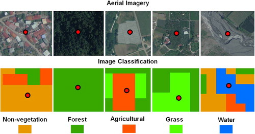
Figure 5. Spatial distributions of land cover types, hydrologic soil group, and CN values of the Chenyoulan watershed in 2008. Source: Author

3.2. Rainfall-runoff events

This study used runoff events of natural precipitation as the basis for runoff analysis. The data chosen were rainfall and runoff monitoring data from 2005 to 2009, during which 10 typhoon events occurred, the total rainfall of which ranged between 40.8 and 1419.7 mm, and cumulative runoff ranged between 8.8 and 1152.9 mm. The typhoon events were Typhoon Haitang (July 16, 2005), Typhoon Longwang (September 30, 2005), Typhoon Bilis (July 12, 2006), Typhoon Sepat (August 16, 2007), Typhoon Krosa (October 5, 2007), Typhoon Kalmaegi (July 16, 2008), Typhoon Fung-wong (July 26, 2008), Typhoon Sinlaku (September 11, 2008), Typhoon Morakot (August 5, 2009), and Typhoon Parma (October 3, 2009). In this study, CN values based on land cover types were used to simulate the runoff in the typhoon events, and then the values were compared with actual monitoring data, as shown in Table 3. Among the 10 typhoon events, five had a 1-year recurrence interval, three had a 2-year recurrence interval, and one had a 3-year recurrence interval. The remaining one, Typhoon Morakot, had an 82-year recurrence interval.

Table 3. Typhoon events and related data.

Typhoon event	Date	Rainfall depth (mm)	Observed runoff depth (mm)	Flood return period (year)
HAITANG	16/07/2005	594.7	528.3	3
LONGWANG	30/09/2005	104.3	20.4	1
BILIS	12/07/2006	408.9	251.9	2
SEPAT	16/08/2007	684.1	487.6	2
KROSA	05/10/2007	503.8	140.3	1
KALMAEGI	16/07/2008	463.2	50.7	1
FUNG-WONG	26/07/2008	308.8	77.7	1
SINLAKU	11/09/2008	824.6	433.8	2
MORAKOT	05/08/2009	1419.7	1152.9	82
PARMA	03/10/2009	40.8	8.8	1

The scale of drainage-basin runoff could be quantified through the conduction of a flow-frequency analysis. Higher flow-recurrence intervals correlated to more substantial effects of the drainage basin on the environment. From 2005–2009, the flow-recurrence interval was primarily between 1 and 3 years. Unfortunately, Typhoon Morakot caused some of the severest damage to the Chenyoulan drainage basin, with a flow-recurrence interval of 82 years. The measured cumulative runoff depth reached 1152.9 mm, impeding the river channel’s ability to successfully drain the flood within a short period of time, thereby causing severe damage to midstream and downstream areas.

3.3. Model verification

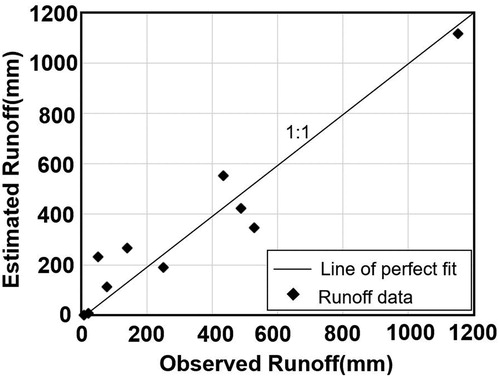
The mean runoff depth of each event was estimated based on the CN method in the SCS manual, which was developed on the basis of hydrologic and antecedent moisture conditions. Figure 6 shows the relationship between the simulated (estimated) and monitored (observed) runoff values in the typhoon events based on the NRCS-CN method. The NSE assessment revealed an NSE value of up to 90.8%, indicating the NRCS-CN method was efficient in predicting the mean runoff depth in the Chenyoulan watershed.

Figure 6. Relationship between observed and estimated runoff depths. Source: Author

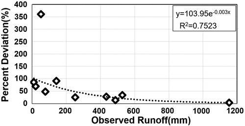
Because numerous studies have attached excess importance to the significance of NSE and overlooked the standard deviation of estimated values from observed values, this study focused on examining the deviation between the two, as shown in Figure 7. Typhoon Sepat, which had a low runoff, had a deviation as high as 359.9%. However, deviation gradually decreased as runoff increased, and the deviation for Typhoon Morakot, which had a high runoff, was only 12.8%. This indicates that the proposed model had a low accuracy when simulating low-runoff events. Despite its favorable performance in the NSE, it was ineffective in mitigating errors when runoff was low. Therefore, follow-up studies are advised against relying solely on the NSE; accuracy at low runoffs should be investigated.

Figure 7. Percent deviation between observed and estimated runoff values. Souce: Author

3.4. Model modification

To address the problem of relatively large errors in the prediction of the low-flow occurrence in small-scale precipitation events, this study involved investigation from two perspectives: initial abstraction (Ia) and CN value analysis unit. Ia in the NRCS-CN method is clearly defined in the National Engineering Handbook 4 (NRCS 1972).

Ia primarily consists of interception, infiltration, and surface-depression storage. Interception and surface-depression storage can be calculated using land-cover and surface conditions. However, the influence of several factors, such as rainfall intensity, soil crusting, and soil moisture, complicate the infiltration process before a storm and thus increase the difficulty of establishing a relationship equation for estimating Ia. Therefore, the original CN method assumes Ia to be a function of maximum potential retention (S). The relationship between Ia and S can be expressed as Ia = 0.2S. This definition of Ia reveals that 0.2 is an experiential coefficient. However, because factors affecting infiltration are complicated, modification of the Ia coefficient becomes a challenge. The present study therefore performed modification using the CN analysis unit.

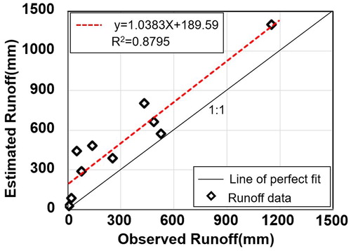
The unit of analysis is critical in runoff estimations using CN values. Numerous studies have used the mean CN of entire watersheds as the unit of analysis, which diluted the accuracy of their findings, resulting in a poor fit between estimated and observed values. This underscores the need for an improved analytic method. Therefore, this study employed the estimated values of the grids the monitoring stations were located in to form a relationship curve with observed values (Figure 8). The results corresponded to a coefficient of determination of 0.879. Therefore, runoff modified according to this grid-based curve could improve the model’s accuracy in spatial distribution, and the estimation of flood risk.

Figure 8. Relationship between grid-based estimated values and observed values. Source: Author

3.5. Risk and disaster

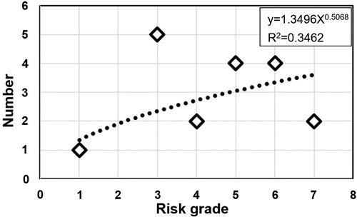
The Chenyoulan watershed is susceptible to flooding when a typhoon or rainstorm event occurs, which has resulted in the scouring of riverbanks, collapse of side slopes, and even headward erosion. These can affect a wide area and take a considerable time to recover, thus hampering economic development, and posing a direct threat to the safety of lives and properties. For this reason, the importance of identifying potential flooded areas quickly, accurately, and at a low cost cannot be overemphasized. This study employed big data of which the hazard and vulnerability data were dynamic and were updated with hydrologic and soil data—for the mapping of flood risk areas. Typhoon Morakot was used as a case study, and its rainfall data were used as the hazard value for runoff depth estimation (Figure 9(b)), which was corrected with monitored data (Figure 9(c)). By contrast, vulnerability data were estimated based on TWIs (Figure 9(d)). Flooding risk was then determined as a probability resulting from the interplay between the hazard and vulnerability values (Figure 9(e)). The assessment of estimated damage and actual damage was conducted by clustering flooding risks into 10 grades. These data were then compared with the sites actually struck by disasters during Typhoon Morakot (Yang et al. 2009). Figure 10 shows the risk grades of the disaster sites, which all fell in the range of 1 − 7. The grading of the flooding risks also provides some insights into the relationship between the flooding risks and number of disaster sites (Figure 11).

Figure 9. Spatial distribution of flooding risks during Typhoon Morakot. (a) Spatial distribution of the potential maximum retention in 2008 (b) Spatial distribution of the runoff during Typhoon Morakot (c) Spatial distribution of the runoff after model revision (d) Spatial distribution of the topographic wetness indices (e) Spatial distribution of Typhoon Morakot-induced flood risks (f) Spatial distribution of the disaster locations. Source: Author

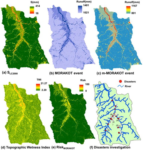
Figure 10. Flooding risk grades of disaster sites during Typhoon Morakot. Source: Author

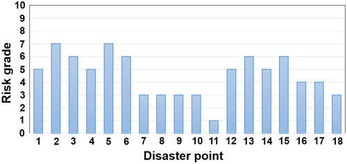
Figure 11. Relationship between flooding risk grades and number of corresponding disaster sites during Typhoon Morakot. Source: Author

3.6. Management strategy

To improve understanding of sites with high flooding risks, the watershed was divided into 101 regions, which were then further clustered into three groups according to their flooding risk (high, moderate, and low). Subsequently, a comparison was made using aerial photographs, and the results are shown in Figure 12. The first group had a high flooding risk, and the regions were mostly sites where river channels converged, which were susceptible to slope collapses induced by scouring along river channels. The second group had a moderate flooding risk, and the regions were mostly sites along mid- to downstream riverbanks, which were susceptible to agricultural and property losses induced by rapid inundation of the riverbanks. The third group had a low flooding risk, and the regions were mostly sites along upstream riverbanks, where the land had largely not been developed or were still virgin forests, and which required no special management measures unless specific hazards occurred or residents required protection. The disaster investigation reported numerous sites in the Chenyoulan watershed had been severely scoured (Figure 9(f) and Table 4) For example, Figure 13 illustrates the effects of a raging torrent, which washed away the foundations of the adjacent road and Long Hua Elementary School. To mitigate the scouring in the Chenyoulan watershed caused by rapidly rising floodwater, which erodes riverbanks and demolishes side slopes, this study proposes buffer zones to be installed as a strategy to counter the impacts on riverbanks (Figure 14). However, this strategy would be highly dependent on the creation of a reasonable buffer zone width, determined based on the runoff depths estimated by the proposed model and the results of terrain analysis.

Figure 12. Hotspots based on analysis of Typhoon Morakot. Source: Author

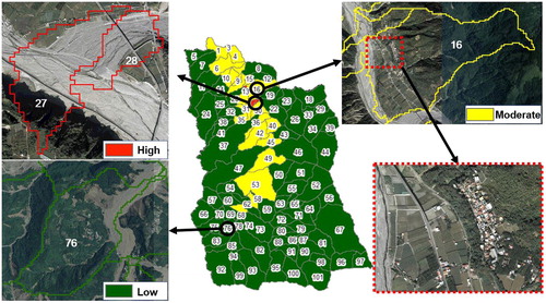
Figure 13. Scouring caused by Typhoon Morakot (Source: Yang et al. 2009).

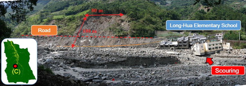
Figure 14. Scouring of riverbanks. Source: Author

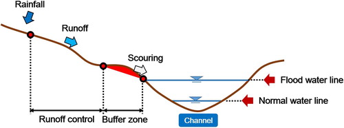
Table 4. Notable disaster sites in the Chenyoulan watershed.

Site	X(m)	Y(m)	Description
A	240775	2608037	Scouring at the toe of the slope along the Habilan rock shed caused extensive slope collapse
B	238250	2609078	Scouring at the toe of the slope below the road caused extensive slope collapse, cutting off the road
C	237370	2607916	Long Hua elementary school was destroyed by a mud slide, forcing the school to be temporarily closed
D	235183	2602756	Collapses and mud slides occurred along several tributaries in the watershed. The mud and rocks that ran down the slopes, which amounted to tens of thousands of cubic meters, destroyed the bridge spanning the Aiyuzi River, cutting access to the outside world
E	2403368	2603974	Scouring of the roadbed along the road temporarily disrupted traffic

Source: Yang et al. 2009.

4. Conclusion

This study investigated the magnitude of runoff during 10 typhoon events between 2005 and 2009, analyzed satellite images, soil maps, and monitoring data, and introduced grid-based parameters into CN values, to enhance the OA of runoff prediction for the Chenyoulan watershed. It was able to draw the following conclusions:

1. For the CN values, this study relied on soil maps and land use data as input parameters. However, because a land use survey would consume considerable labor and resources, and could not be updated in a short timeframe, the study used satellite image classification instead. The feasibility of this approach was tested by comparing the corresponding land cover classifications with aerial photographs, and the results indicated a favorable OA (Kappa coefficient = 0.71).

2. To investigate the accuracy of modeled surface runoff, empirical data of typhoon events were employed, which resulted in an NSE of 90.8%. However, despite the favorable NSE, the model did not reflect the real situation. To counter this deficiency, this study adopted an unconventional approach of adjusting the estimated runoff with the relationship curve (R² = 0.879) based on the estimated values of the grids in which the monitoring stations were located.

3. This study used hazard and vulnerability as indicators for the flood risk model, the results of which were then compared with historical data of the disaster sites. This revealed a positive correlation between flooding risk grade and number of disaster sites. Therefore, the grading of flooding risks can serve as a reference for flood hazard management.

4. Disaster management should cover the management of slopes and river channels. Slope management should be conducted according to the flooding risk. Attention should be paid to regions with moderate to high flooding risks, which are mostly located on the slopes along riverbanks, for sudden rises in water level to avoid agricultural and property losses. In contrast, regions with low flooding risks, which are mostly located in undeveloped lands or virgin forests in midstream or upstream regions, usually do not require special management measures. Establishment of riparian buffer zones is advisable for river channel management to mitigate the scouring that can cause riverbank erosion and side slope collapse.

Acknowledgements

The author would like to express deep and sincere gratitude to Prof. Dr. Chao-Yuan Lin, who has taught and guided me in research.

Disclosure statement

No potential conflict of interest was reported by the authors.

Data availability statement

Not applicable.

References

- Ayanlade A, Howard MT. 2017. Understanding changes in a Tropical Delta: a multi-method narrative of landuse/landcover change in the Niger Delta. Ecol Modell. 364:53–65.
- Chen YM, Su JL, Fan KS. 2009. Disaster risk assessment development trend. J Crisis Manag. 6(1):41–50.
- Cheţan MA, Dornik A, Urdea P. 2018. Analysis of recent changes in natural habitat types in the Apuseni Mountains (Romania), using multi-temporal Landsat satellite imagery (1986–2015). Appl Geogr. 97:161–175.
- Congalton RG. 1991. A review of assessing the accuracy of classification of remotely sensed data. Remote Sens Environ. 37(1):35–46.
- Fan F, Deng Y, Hu X, Weng Q. 2013. Estimating composite curve number using an improved SCS-CN method with remotely sensed variables in Guangzhou, China. Remote Sens. 5(3):1425–1438.
- Fang YK. 2003. Application on land cover classification using normalized difference vegetation indices―a case study at Meinung Zhangtan Area [master thesis]. Pintung City, Taiwan: National Pingtung University of Science and Technology.
- Guru N, Jha R. 2015. Flood frequency analysis of Tel basin of Mahanadi river system, India using annual maximum and POT flood data. Aquat Procedia. 4:427–434.
- Huang M, Gallichand J, Wang Z, Goulet M. 2006. A modification to the soil conservation service curve number method for steep slopes in the Loess Plateau of China. Hydrol Process. 20(3):579–589.
- Janssen LF, Vanderwel JM. 1994. Accuracy assessment of satellite derived land-cover data: a review. Photogramm Eng Remote Sens. 60(4):419–426.
- Jung JW, Yoon KS, Choi DH, Lim SS, Choi WJ, Choi SM, Lim BJ. 2012. Water management practices and SCS curve numbers of paddy fields equipped with surface drainage pipes. Agric Water Manag. 110:78–83.
- Lee CT. 1996. A geomorphological view to the disaster the chenyulan creek during the herb typhoon. Sino-Geotechnics 57:17–24.
- Lee HS, Yamashita T, Hsu JRC, Ding F. 2013. Integrated modeling of the dynamic meteorological and sea surface conditions during the passage of Typhoon Morakot. Dyn Atmos Oceans. 59:1–23.
- Li H, Zhang Y. 2017. Regionalising rainfall-runoff modelling for predicting daily runoff: comparing gridded spatial proximity and gridded integrated similarity approaches against their lumped counterparts. J Hydrol. 550:279–293.
- Lin CY. 2012. Watershed land cover classification and hotspot monitoring using environmental index [master thesis]. Taichung City, Taiwan: National Chung Hsing University.
- Lin CY, Chou WC, Lin WT. 2002. Modeling the width and placement of riparian vegetated buffer strips: a case study on the Chi-Jia-Wang Stream, Taiwan. J. Environ Manag. 66:269–280.
- Lin CY, Lin HJ, Liou CW. 2004. Establishment of a dynamic analysis system for rainfall-runoff hydrograph analysis in Chenyulan Creek watershed. J Soil Water Conserv. 36(3):243–258.
- Nash JE, Sutcliffe JE. 1970. Modeling infiltration during steady rain. Water Resour Res. 9:384–394.
- Natural Resources Conservation Service (NRCS). 1972. National engineering handbook (Section 4, Hydrology). Washington (DC): U.S. Government Printing Office.
- Ozdemir H, Elbaşı E. 2015. Benchmarking land use change impacts on direct runoff in ungauged urban watersheds. Phys Chem Earth A/B/C. 79–82:100–107.
- Sörensen R, Zinko U, Seibert J. 2006. On the calculation of the topographic wetness index: evaluation of different methods based on field observations. Hydrol Earth Syst Sci. 10(1):101–112.
- Swinbourne MJ, Taggart DA, Swinbourne AM, Lewis M, Ostendorf B. 2018. Using satellite imagery to assess the distribution and abundance of southern hairy-nosed wombats (Lasiorhinus latifrons). Remote Sens Environ. 211:196–203.
- Tung YT, Pai TY. 2015. Water management for agriculture, energy, and social security in Taiwan. Clean Soil Air Water. 43(5):627–632.
- United Nations Disaster Relief Organization (UNDRO). 1979. Natural disasters and vulnerability analysis, report of the expert group meeting. Geneva: UNDRO.
- Yang MD, Lin JY, Lin WJ, Huang KS, Wu DY. 2009. Disaster investigation in Chenyulan river basin during Typhoon Morakot. J Chin Soil Water Conserv. 40(4):345–358.
- Yang TH, Yang SC, Ho JY, Lin GF, Hwang GD, Lee CS. 2015. Flash flood warnings using the ensemble precipitation forecasting technique: a case study on forecasting floods in Taiwan caused by Typhoons. J Hydrol. 520:367–378.