Two novel neural-evolutionary predictive techniques of dragonfly algorithm (DA) and biogeography-based optimization (BBO) for landslide susceptibility analysis

Abstract

Due to the wide application of evolutionary science in different engineering problems, the main aim of this paper is to present two novel optimizations of multi-layer perceptron (MLP) neural network, namely dragonfly algorithm (DA) and biogeography-based optimization (BBO) for landslide susceptibility assessment at a study area, West of Iran. Utilizing 14 landslide conditioning factors, namely elevation, slope aspect, plan curvature, profile curvature, soil type, lithology, distance to the river, distance to the road, distance to the fault, land cover, slope degree, stream power index (SPI), and topographic wetness index (TWI) and rainfall as the input variables, and 208 historical landslides as target variable, the required spatial database is created. Then, the MLP is synthesized with the mentioned algorithms to develop the proposed DA-MLP and BBO-MLP ensembles. Three accuracy criteria of mean square error, mean absolute error, and area under the receiving operating characteristic curve are used to evaluate the performance of the models and also to develop a score-based ranking system. As the first outcome, the application of the DA and BBO metaheuristic algorithms enhances the accuracy of the MLP. Moreover, referring to the calculated total ranking scores of 6, 14, and 16, it was revealed that the BBO performs more efficiently than DA in optimizing the MLP.

Keywords:

• Landslide susceptibility mapping
• artificial neural network
• DA algorithm
• BBO algorithm

Introduction

As a frequent and ubiquitous natural hazard, landslides are described as downward mass movements (triggered by gravity), and as a consequent of anthropogenic and natural activities (Varnes and Radbruch-Hall 1976; Cruden 1991; Aksoy et al. 2016; Aksoy and Gor 2017; Bui et al. 2019; Moayedi, Bui, et al. 2019). Due to undesirable impacts of this environmental threat on urbanization and environmental developments, studying the landslides has received a growing attraction from the side of international scientific community (Aleotti and Chowdhury 1999; Tsangaratos and Ilia 2016). Globally, the vast majority (more than 90%) of the landslides have occurred in developing countries, and they are responsible for around 17% of the reported fatalities (Pourghasemi et al. 2012). In Iran, the landslides have caused more than 185 loss of lives. Considering the distribution of the historical landslide events, the western part of Iran is known as a landslide-prone region. Seimareh landslide (occurred in Lorestan Province), for example, it was the largest debris flow observed worldwide (Shoaei and Ghayoumian 1998). Therefore, analysing the landslide susceptibility is a crucial prerequisite in facing this phenomenon (Hong et al. 2019).

Due to the involvement of various geo-environmental causative factors, investigating the landslide susceptibility entails establishing complex and non-linear relationships. So far, many studies have conducted proper landslide susceptibility mapping using statistical techniques (Youssef et al. 2015; Chen et al. 2016; Razavizadeh et al. 2017). Also, multi-criteria decision models have shown good capability in this field (Kumar and Anbalagan 2016; Myronidis et al. 2016). In a comparative study, Nicu (2018) employed analytic hierarchy process (AHP), statistical index (SI), and frequency ratio (FR) for landslide susceptibility mapping in Romania. It was found that all three models achieve the prediction rate higher than 50%. However, the AHP (with around 80% accuracy in both training and testing phases) outperforms two other used approaches.

According to Pradhan (2013), utilizing machine learning tools are one of the most effective strategies suggested for analysing the relationship between the landslide and conditioning factors. These models have also shown high robustness for other environmental modelling like flood (Mojaddadi et al. 2017; Termeh et al. 2018) and groundwater contamination (Rizeei et al. 2018). In this sense, Pourghasemi, Jirandeh, et al. (2013) showed the efficiency of support vector machine by testing different kernel classifiers for landslide susceptibility assessment in Golestan Province of Iran. Similarly, Oh and Pradhan (2011) showed the efficiency of adaptive neuro-fuzzy inference system (ANFIS) for regional landslide susceptibility mapping in a prone district of Penang Island, Malaysia. Moreover, many studies have successfully used artificial neural network (ANN) for discerning the spatial relationship between landslide and its conditioning factors (Lee et al. 2004; Kawabata and Bandibas 2009; Can et al. 2019; Tian et al. 2019). Yilmaz (2009) showed the superiority of the ANN when is compared with FR and logistic regression (LR) models. Accordingly, area under the curve (AUC) of the used models was 0.852, 0.826, and 0.842, respectively for the ANN, FR, and LR.

Looking for more powerful evaluative tools, many scholars have suggested the use of hybrid metaheuristic algorithms (Jaafari et al. 2019; Nguyen, Mehrabi, et al. 2019). More clearly, utilizing typical intelligent models is associated with some computational drawbacks like local minimum (Moayedi et al. 2018). Optimization algorithms enhance the accuracy of these tools by overcoming the mentioned problems (Chen et al. 2017; Gao, Dimitrov, et al. 2018; Gao, Wang, et al. 2018; Gao et al. 2019; Moayedi, Mehrabi, et al. 2019). Bui et al. (2017) used artificial bee colony optimization technique for determining proper set of hyper-parameters of least squares support vector machines (LSSVM) in spatial analysis of rainfall-triggered landslides at Lao Cai area, Vietnam. With 90% accuracy, the susceptibility map produced by the proposed model was more accurate than which produced by the typical SVM prediction. Likewise, Tien Bui et al. (2018) used imperialist competitive algorithm (ICA) for optimizing relevance vector machine (RVM) to produce the landslide susceptibility map of Lang Son city of Vietnam. Their findings indicated that the suggested RVM-ICA (AUC = 0.92) performs more efficiently than two benchmarks, namely the SVM (AUC = 0.91) and LR (AUC = 0.87).

The focal point of this paper is to present two novel optimizations of the ANN, namely dragonfly algorithm (DA) and biogeography-based optimization (BBO) for landslide susceptibility mapping at a landslide-prone area, West of Iran. Although various optimization techniques have been applied to intelligent models, the authors did not come across any precedent study focused on combining the DA and BBO with ANN for the mentioned purpose. This is worth noting that the main contribution of these algorithms to the spatial analysis of the landslide susceptibility is finding the most appropriate computational parameters of the ANN which are assigned to the conditioning factors.

Study area

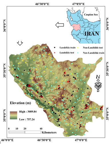
The study area is located between the longitude 46° 00′ to 47° 20′E, and the latitude 34° 45′ to 35° 48′N, West of Iran (Figure 1). It covers an area of nearly 7811 km². The study area is known as a mountainous area with around 500 mm of average annual precipitation. Two major climates in this region are humid weather and the Mediterranean warm, which results in heavy rainfalls and snowfalls (Shirzadi, Bui, et al. 2017). Our proposed area comprises three cities of ‘Marivan’, ‘Sanandaj’, and ‘Kamyaran’. The altitude ranges approximately from 750 to 3100, and the maximum terrain slope is about 60%. The land is mostly covered by good ranges, and the economy of the inhabitants is significantly influenced dependent on dry farming and irrigated agriculture (Rahmati et al. 2015). According to the lithology map, 40 different lithology units are found there, where ‘Dark grey argillaceous shale’ is the most common one, covering around 18% of the area. Moreover, five soil groups can be found, namely ‘Inceptisols’, ‘Rock Outcrops/Entisols’, ‘Rock Outcrops/Inceptisols’, ‘Water Body’, and ‘Entisols/Inceptisols’, where the majority of the area (around 80%) is covered by the second soil group.

Figure 1. Location of the study area and spatial distribution of the landslides.

Data preparation and spatial interaction between the landslide and conditioning factors

When it comes to artificial intelligence techniques, the used dataset consists of two types of parameters, including a target variable, influenced by one or more independent variable(s). In this research, the landslide inventory map plays the role of the target variable, and the input variables were 14 landslide conditioning factors, including elevation, slope aspect, plan curvature, profile curvature, soil type, lithology, distance to the river, distance to the road, distance to the fault, land cover, slope degree, stream power index (SPI), and topographic wetness index (TWI) and rainfall. These layers were created and processed in geographic information system (GIS) with a pixel size of 10 × 10 m (Pradhan et al. 2010; Shirzadi, Shahabi, et al. 2017; Vakhshoori and Pourghasemi 2018). A total of 208 historical landslide events were identified by using previous records (Shirzadi, Bui, et al. 2017; Mezaal et al. 2018; Mojaddadi Rizeei et al. 2019; Rizeei and Pradhan 2019) as well as interpreting the aerial photos (in 1:25,000 scale), supported by field monitoring. It is worth noting that, typologically, the marked landslides were mostly rotational slides. Therefore, based on the landslide classification of Varnes (1978), other types of slope failures suchlike translational slides, flow, and lateral spreading were eliminated (Nguyen, Bui, et al. 2019). The same number of non-landslide points were then randomly created over the areas devoid of the landslide. Also, in order to explore the spatial relationship between the landslide and its conditioning factors, the FR theory is used. In this method, the correlation between each sub-group and landslide is directly proportional to the magnitude of the calculated FR (Oh et al., 2011). Let N_landslide and N_domain stand for the percentage of the landslides marked in the proposed sub-group and the percentage of the terrain covered by it, respectively; then the FR is calculated as follows: (1) $$FR=\mathrm{ }\frac{N_{\mathrm{landslide}}}{N_{\mathrm{domain}}}$$(1)

Figure 2 portrays the map of each conditioning factors along with the obtained FRs. Moreover, Table 1 presents the description of the lithological units (Figure 3), as well as the calculated FRs. As these charts and the table denote, the categories of (1000–1500) m for elevation, North (0–22.5°) for slope aspect, ‘Concave’ for plan curvature (0.001–1.1576e + 10) for profile curvature, ‘Inceptisols’ for soil type (100–200) m for distance to the river (200–300) m for distance to the road (300–400) for distance to the fault, ‘Agriculture’ for land cover (10–15) degrees for slope (85e5–23e6) for SPI (−9.38 to −7.40) for TWI (500–600) mm for rainfall, and ‘Jugr’ for lithology are the most correlated sub-groups, due to the largest FRs obtained for them.

Figure 2. The calculated FR for: (a and b) elevation, (c and d) slope aspect, (e and f) plan curvature, (g and h) profile curvature, (i and j) soil type, (k and l) distance to river, (m and n) distance to road, (o and p) distance to fault, (q and r) land cover, (s and t) slope degree, (u and v) SPI, (w and x) TWI, and (y and z) rainfall.

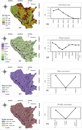
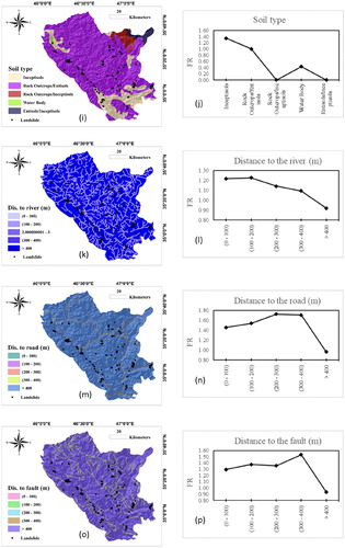
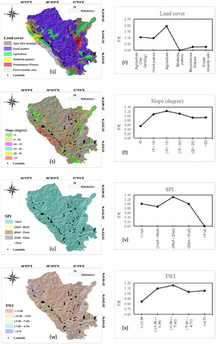
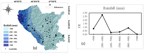
Figure 3. The lithology of the study area.

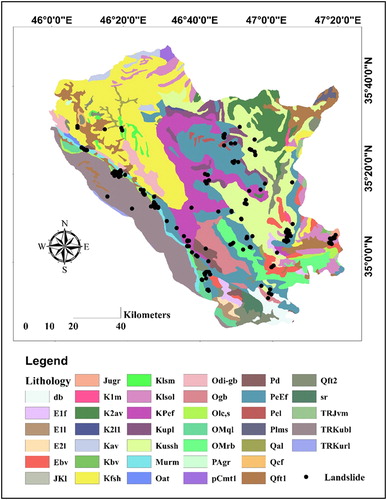
Table 1. The description of the lithology units.

Symbol	Description	Age	Age era	FR
Qft1	High-level piedmont fan and valley terrace deposits	Quaternary	CENOZOIC	0.32
OMql	Massive to thick-bedded reefal limestone	Oligocene-Miocene	CENOZOIC	5.94
pCmt1	Medium-grade, regional metamorphic rocks (amphibolite facies)	Pre-Cambrian	PROTEROZOIC	0.00
Kav	Andesitic volcanic	Late Cretaceous	MESOZOIC	0.00
Kfsh	Dark grey argillaceous shale	Cretaceous	MESOZOIC	0.11
K1m	Limestone, argillaceous limestone; tile red sandstone and gypsiferous marl	Early Cretaceous	MESOZOIC	0.00
Plms	Marl, shale, sandstone and conglomerate	Pliocene	CENOZOIC	0.00
Klsm	Marl, shale, sandy limestone and sandy dolomite	Early Cretaceous	MESOZOIC	2.20
Qft2	Low-level piedmont fan and valley terrace deposits	Quaternary	CENOZOIC	0.45
E2l	Nummulitic limestone	Eocene	CENOZOIC	0.00
Klsol	Grey thick-bedded to massive orbitolina limestone	Early Cretaceous	MESOZOIC	0.95
K2av	Andesitic volcanic	Late Cretaceous	MESOZOIC	0.00
Murm	Light-red to brown marl and gypsiferous marl with sandstone intercalations	Miocene	CENOZOIC	5.74
Pd	Red sandstone and shale with subordinate sandy limestone (DORUD FM)	Permian	PALEOZOIC	0.84
Qal	Stream channel, braided channel and flood plain deposits	Quaternary	CENOZOIC	0.00
PAgr	Granite	Paleocene-Eocene	CENOZOIC	0.00
TRKurl	Purple and red thin-bedded radiolarian chert with intercalations of neritic and pelagic limestone (Kerman and Neyzar Radiolarites)	Triassic-Cretaceous	MESOZOIC	0.00
Kussh	Dark grey shale (Sanandaj shale) (Schist and phyllite)	Late Cretaceous	MESOZOIC	1.24
Olc,s	Conglomerate and sandstone	Oligocene	CENOZOIC	6.83
Ebv	Basaltic volcanic rocks	Middle Eocene	CENOZOIC	3.75
Odi-gb	Diorite to gabbro	Oligocene	CENOZOIC	0.00
PeEf	Flysch turbidite, sandstone and calcareous mudstone	Paleocene-Eocene	CENOZOIC	1.83
Qcf	Clay flat	Quaternary	CENOZOIC	0.22
Kupl	Globotrunca limestone	Late Cretaceous	MESOZOIC	0.73
K2l1	Hyporite-bearing limestone (Senonian)	Late Cretaceous	MESOZOIC	0.00
KPef	Thinly bedded sandstone and shale with siltstone, mudstone limestone and conglomerate	Late Cretaceous- Paleocene	MESOZOIC- CENOZOIC	0.98
TRKubl	Kuhe Bistoon limestone	Triassic-Cretaceous	MESOZOIC	0.85
Oat	Andesitic tuff	Oligocene	CENOZOIC	0.89
Pel	Medium to thick-bedded limestone	Paleocene-Eocene	CENOZOIC	2.30
TRJvm	Meta-volcanics, phyllites, slate and meta-limestone	Triassic-Jurassic	MESOZOIC	0.00
JKl	Crystalized limestone and calc-schist	Jurassic-Cretaceous	MESOZOIC	0.00
Kbv	Basaltic volcanic	Early Cretaceous	MESOZOIC	0.00
Jugr	Upper Jurassic granite including Shir Kuh Granite and Shah Kuh Granite	Late Jurassic	MESOZOIC	10.90
Ogb	Gabbro	Oligocene	CENOZOIC	0.34
OMrb	Red Beds composed of red conglomerate, sandstone, marl, gypsiferous marl and gypsum	Oligocene-Miocene	CENOZOIC	0.71
pd2	Peridotite including harzburgite, dunite, lherzolite and websterite	Triassic-Cretaceous	MESOZOIC	1.02
E1f	Silty shale, sandstone, marl, sandy limestone, limestone and conglomerate	Early Eocene	CENOZOIC	0.88
db	Diabase	Late Cretaceous	MESOZOIC	0.00
sr	Serpentinite	Triassic-Cretaceous	MESOZOIC	0.00
E1l	Nummulitic limestone	Eocene	CENOZOIC	0.00

Methodology

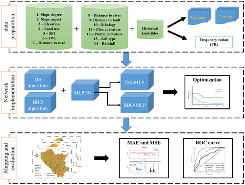
Acceding to Figure 4, the overall methodology of this research can be presented in three major steps. Firstly, the spatial database consisting of landslide inventory map as well as 14 landslide conditioning layers is provided, then the identified landslide points are randomly divided into the training (i.e. 70% or 146 landslides) and testing (the remaining 30% or 62 landslides) parts. Note that, the first group is devoted to develop and train the intelligent models, and the second group is used as unseen landslides to evaluate the accuracy of the implemented models. After that, the MLP (multi-layer perceptron) is coupled with the DA and BBO evolutionary algorithms to develop the DA-MLP and BBO-MLP neural ensembles. Lastly, after generating the landslide susceptibility maps, the performance of the models is evaluated by three accuracy criteria, namely mean square error (MSE), mean absolute error (MAE), and area under the receiving operating characteristic curve (AUROC). Equations (2)(2) $$\mathit{MSE}=\mathrm{ }\frac{1}{N}\sum _{i=1}^N{(Y_{i_{\mathit{observed}}}-Y_{i_{\mathit{predicted}}})}^2$$(2) and (3)(3) $$\mathit{MAE}=\mathrm{ }\frac{1}{N}\sum _{i=1}^N(Y_{i_{\mathit{observed}}}-Y_{i_{\mathit{predicted}}})$$(3) express the formula of the MSE and MAE: (2) $$\mathit{MSE}=\mathrm{ }\frac{1}{N}\sum _{i=1}^N{(Y_{i_{\mathit{observed}}}-Y_{i_{\mathit{predicted}}})}^2$$(2) (3) $$\mathit{MAE}=\mathrm{ }\frac{1}{N}\sum _{i=1}^N(Y_{i_{\mathit{observed}}}-Y_{i_{\mathit{predicted}}})$$(3) in which N shows the number of involved samples, and $Y_{i_{\mathit{observed}}\mathrm{ }}$ and $Y_{i_{\mathit{predicted}}\mathrm{ }}$ are the desired and predicted values of landslide susceptibility, respectively.

Figure 4. Applied procedure for landslide susceptibility assessment of this study.

Here, the used intelligent models are described:

Artificial neural network

Mimicking the connecting behaviour of the biological neural networks, the idea of ANN was first presented by McCulloch and Pitts (1943). The ability of non-linear analysis has made the ANNs capable tools for input-output mapping of a set of data samples (ASCE Task Committee 2000). Different types of ANNs have been promisingly used for simulating various engineering problems (Moayedi and Rezaei 2017; Moayedi and Hayati 2018a, 2018b; Azeez et al. 2019). MLP is one of the most regularly used types of ANNs which is composed of at least three layers which contain the main processor units (see Figure 5). It has been stated that one hidden layer is sufficient for neural modelling of any problem (Cybenko 1989; Hornik et al. 1989).

Figure 5. The general structure of the ANN.

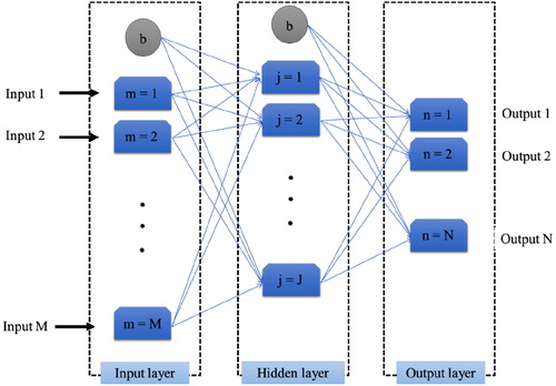
During the ANN implementation, let I = {$a_i,$ $b_i,$ $c_i$ …; i = 1, 2, … K} and O = {${\alpha }_i,$ ${\beta }_i,$ ${\gamma }_i$ …; i = 1, 2, … K} be the input and output vectors, respectively. Then, the response of the jth node is calculated as follows: (4) $$O_j=F\mathrm{ }\left(\mathrm{ }\sum _{m=1}^M(I_{m\mathrm{ }}{W}_{mj}\right)+b_{j\mathrm{ }})$$(4) in which W and b stand for the weight and bias. Also, F symbolizes the activation function that is set to be hyperbolic tangent sigmoid (Tansig) in this study: (5) $$\mathrm{Tansig}(x)=\frac{2}{1+e^{-2x}}-1$$(5)

Dragonfly algorithm

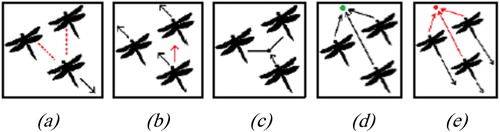
The DA has been proposed as a proper algorithm for optimization tasks (such as adjusting the ANN synaptic weights). Mirjalili (2016) proposed this algorithm for the first time. It is an algorithm that inspired using the static and dynamic conducts of dragonflies. In the life cycle of dragonflies, there are two different stages including (i) the nymph stage which forms most of their cycle of life and (ii) transformation to the adult stage.

The stationary behaviour of dragonflies is the same as the utilization stage in meta-heuristics (Russell et al. 1998). From a different aspect, the dynamic conduct is same to the exploration stage that is where they enter to groups and fly aboard of various zones to discover food resources (Wikelski et al. 2006). The DA is derived by the Reynolds Swarm Intelligence. It draws on around five distinct principles, which are fundamental in discovering the solution of weights.

1. The separation origin has been known as the collision digression of a dragonfly of other dragonflies, which are near its zone (Figure 6(a)).

2. The alignment origin shows velocity conforming of a dragonfly for other different dragonflies, which are near to zone (Figure 6(b)).

3. The cohesion origin is considered as the trend of a dragonfly to the space centre and includes other dragonflies near to its location (Figure 6(c)).

4. Whereas the basic aim of dragonfly swarms is to survive, attraction to food origin (Figure 6(d)) shows that dragonflies have to move near food sources.

5. The distraction from enemies’ origins (Figure 6(e)) occurs when dragonflies run far away from the enemy sources for surviving (Mirjalili 2016).

Figure 6. Different stages of the DA (after Yasen et al. 2018).

By Equation (6)(6) $$S_i=-\sum _{j=0}^{n}X-X_j$$(6) , we can calculate the separation value. X shows the current dragonfly position, X_j stands for the of the jth dragonfly position near X, n indicates the dragonflies number. The alignment amount can be computed by Equation (7)(7) $$A_i=-\frac{{\sum }_{j=0}^n{V}_j}{n}$$(7) . The term Vj shows the velocity of jth dragonfly near the current one. The cohesion amount can be computed by Equation (8)(8) $$C_i=-\frac{{\sum }_{j=0}^n{X}_j}{n}-X$$(8) . The attraction to food from dragonflies can be computed by Equation (9)(9) $$F_i=X^f-X$$(9) . X^f stands for the food source position. The confusion of enemy amount can be predicted by Equation (10(10) $$E_i=X^e-X$$(10) ). X^e shows the enemy position. To update the dragonflies position for examining different weight solution as well as possess another fitness amount, ΔX and X have been computed by Equations (11)(11) $$\Delta X_{i.j}=\left(s{S}_j+a{A}_j+c{C}_j+f{F}_j+e{E}_j\right)+w\mathrm{ }\Delta X_{i-1.j-1}$$(11) and (12)(12) $$X_{i.j}=X_{i-1.j-1}+\mathrm{ }\Delta X_{i.j}$$(12) (Mirjalili 2016): (6) $$S_i=-\sum _{j=0}^{n}X-X_j$$(6) (7) $$A_i=-\frac{{\sum }_{j=0}^n{V}_j}{n}$$(7) (8) $$C_i=-\frac{{\sum }_{j=0}^n{X}_j}{n}-X$$(8) (9) $$F_i=X^f-X$$(9) (10) $$E_i=X^e-X$$(10) (11) $$\Delta X_{i.j}=\left(s{S}_j+a{A}_j+c{C}_j+f{F}_j+e{E}_j\right)+w\mathrm{ }\Delta X_{i-1.j-1}$$(11) (12) $$X_{i.j}=X_{i-1.j-1}+\mathrm{ }\Delta X_{i.j}$$(12) in which, a, s, e, f, c, e, and w are the weights of their related element.

Biogeography-based optimization

BBO is a population-based search method which was developed according to the biogeography theory (Simon 2008). Mirjalili et al. (2014) coupled this algorithm with a MLP neural network for the first time. The flowchart of the BBO is presented in Figure 7. Similar to other evolutionary techniques, at the first step of the BBO, a random population is produced named ‘habitat’. Two parameters of habitat suitability index (HSI) and suitability index variable (SIV) are defined to evaluate the goodness of these individuals (i.e. possible solutions) and the habitability of the habitats and areas. The BBO originally includes two operations, namely migration and mutation that are briefly explained in the following (Hadidi 2015).

Figure 7. The flowchart of the BBO algorithm.

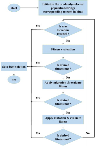
Firstly, the possible solutions are modified in order to enhance their goodness. In this phase, to decide whether the modification of the SIVs is necessary or not, an immigration rate (λg) is defined (Bhattacharya and Chattopadhyay 2010). In the cases where the modification is required, an emigration rate (μg) is defined. It is used to probabilistically determine the solution that will migrate. This is worth noting that the algorithm keeps away the highly fitted solutions to prevent probabilistic corruption (Roy et al. 2010).

As is known there are various natural hazards which threaten a geographical area. Hence, it is likely to observe some abrupt changes in HIS values. Consequently, during the mutation process, the habitat might deviate from its equilibrium HIS. In this stage, a probability factor is calculated for each relation of the population decide whether it needs to mutate or not. Moreover, this factor determines the solution to the existing problem. In this sense, the more value of probability, the more closeness to the overall solution (Hadidi 2015). Let S be the number of species, then, the rate of mutation is expressed as follows: (13) $$P_g^f=\{\begin{array}{l}-({\lambda }_g+{\mu }_g)P_g+{\mu }_{g+1}{P}_{g+1}\mathit{\text{ S}}=0,\\ -({\lambda }_g+{\mu }_g)P_g+{\lambda }_{g-1}{P}_{g-1}+{\mu }_{g+1}{P}_{g+1}1\le S\le S_{\max }-1,\\ -({\lambda }_g+{\mu }_g)P_g+{\lambda }_{g-1}{P}_{g-1}\mathit{\text{ S}}=S_{\max }.\end{array}$$(13)

Results and discussion

Model implementation

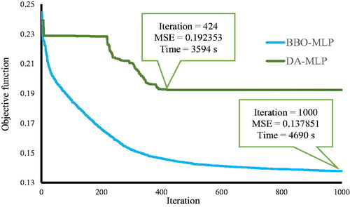
As mentioned previously, this paper outlines two metaheuristic optimization of the neural intelligence for the problem of landslide susceptibility. To do this, the DA and BBO techniques are synthesized with a MLP neural network to enhance its prediction capability. More specifically, the solutions that are suggested by these algorithms contain the optimized values of the weights and biases of the MLP. Therefore, it needs to be mathematically introduced to the algorithms. This process was carried out by the assist of the programming language of MATLAB 2014. The proposed DA-MLP and BBO-MLP networks were implemented with population size of 250 and 1000 repetitions. Also, the MSE was defined as the objective function (OF) to measures the performance error at the end of each iteration. The convergence curves of the implemented models are presented in Figure 8. As can be seen, there are some significant distinctions between the optimization behaviours of the DA and BBO algorithms. Although the maximum value of the OF is between 0.23 and 0.25 for both of them, the BBO continues decreasing error until the last repetition. This is while in DA, the majority of the error reduction has occurred between 220 and 424th repetitions. Also, at the end of the process, the training error of the DA-MLP and BBO-MLP reaches to 0.1923 and 0.1378, respectively.

Figure 8. The convergence cure of the applied DA-MLP and BBO-MLP models.

Landslide susceptibility mapping

After developing the DA-MLP and BBO-MLP predictive ensembles, the calculated landslide susceptibility values were transformed into the GIS environment to produce the susceptibility maps of each model. Next, based on these values, the study area was divided into five susceptibility classes, namely ‘Very low’, ‘Low’, ‘Moderate’, ‘High’, and ‘Very high’ (Xi et al. 2019). It was done by using natural break classification method which tries to reduce the variance within classes and maximize the variance between classes (Jenks 1967; Liu and Duan 2018). The main reason for selecting natural break was the highest popularity of this method for this aim (Irigaray et al. 2007; Akgun et al. 2012; Xu et al. 2012; Pourghasemi, Pradhan, et al. 2013; Jaafari et al. 2014; Gao, Guirao, et al. 2018; Gao, Wu, et al. 2018). Also, it is proper to note that other existing methods, like equal interval and quantile method, have some weaknesses for being used in such works (Ayalew et al. 2004; Tehrany et al. 2019). The resulted maps are shown in Figure 9(a–c), respectively for the typical MLP, DA-MLP, and BBO-MLP prediction.

Figure 9. Landslide susceptibility maps generated by (a) typical MLP, (b) DA-MLP, and (c) BBO-MLP models.

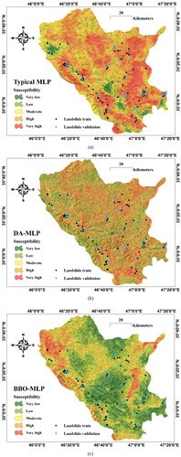
The percentage of the area covered by each susceptibility category is calculated and presented in Table 2. As the table denotes, the MLP has classified 71.02% (around 5548 km²) of the area as hazardous regions (i.e. under the High and Very high susceptibility). This value is obtained as 50.06% (around 3911 km²) and 23.51% (around 1836 km²) by the DA-MLP and BBO-MLP, respectively. At the same time, considering the safe areas (i.e. Very low susceptibility class), it can be deduced that the MLP has presented more cautious prediction. In this regard, 3.07%, 11.67% and 20.99% of the area is recognized by the least landslide susceptibility.

Table 2. The ratio and area of each susceptibility class.

Susceptibility class	MLP		DA-MLP		BBO-MLP
	Ratio (%)	Area (km^2)	Ratio (%)	Area (km^2)	Ratio (%)	Area (km^2)
Very low	3.07	239.64	11.67	911.51	20.99	1639.98
Low	5.72	446.55	18.61	1453.90	31.59	2467.69
Moderate	20.19	1577.30	19.66	1535.54	23.91	1867.45
High	42.14	3291.51	22.82	1782.73	16.70	1304.26
Very high	28.89	2256.45	27.24	2127.77	6.81	532.07
Hazardous regions	71.02	5547.96	50.06	3910.50	23.51	1836.33

Performance assessment of the models

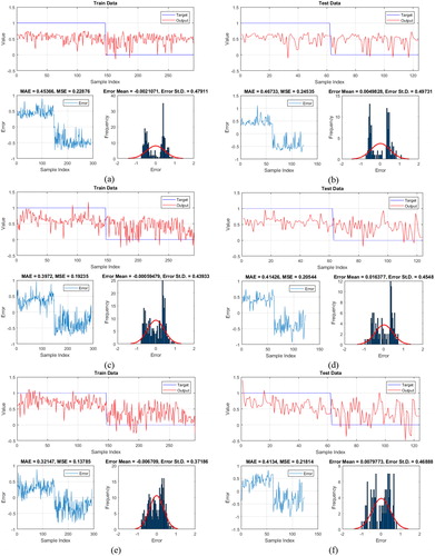
The performance assessment of the implemented models consists of two parts. Statistically, the MSE and MAE are defined to measure the training and testing error of the implemented MLP, DA-MLP, and BBO-MLP. The results are portrayed in Figure 10, showing a graphical comparison between the predicted and observed landslide susceptibility indices, as well as the histogram of the errors. According to these figures, synthesizing the MLP with the DA and BBO evolutionary techniques has effectively helped it to enjoy more learning and prediction capability of landslide pattern. More clearly, in the training phase, the MSE experienced a decrease by around 16% and 40% as the result of applying the DA and BBO algorithms, respectively. About the MAE, it was reduced by around 12% and 29%. As for the testing phase, the DA was more successful than BBO, in terms of decreasing the MSE (nearly 11% vs. 16%). But the MAE results show a slightly lower mean absolute error for the BBO products (0.4134 vs. 0.4142).

Figure 10. The results obtained for the (a and b) MLP, and (c and d) DA-MLP, and (e and f) BBO-MLP, respectively for the training and testing samples.

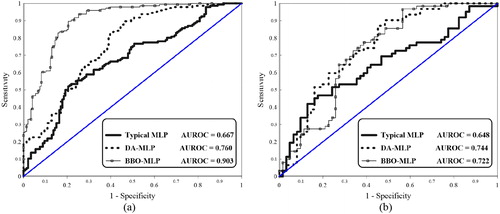
The third considered criterion is the area under the receiver operating characteristic curves (AUROC) which measures the accuracy of the developed susceptibility maps. In this regard, many studies have recommended the ROC curves for evaluating the predictions related to diagnostic problems (Egan 1975), like natural hazards (Beguería 2006). When it comes to landslide susceptibility modelling, the ROC shows the proportion of the non-landslide grid cells which are correctly labelled ‘no-failure’ (i.e. the specificity) versus the proportion of the landslide grid cells which are correctly labelled ‘failure’ (i.e. the sensitivity) (Swets 1988; Lasko et al. 2005; Beguería 2006). The obtained ROC curves of both training and testing phases of the MLP, DA-MLP, and BBO-MLP models are presented in Figure 11(a,b), respectively. As the figures point out, the results are in a good agreement with the calculated MSE and MAE indices. The training accuracy of the typical MLP has considerably increased from 66.7% to 76% and 90.3%, respectively by applying the DA and BBO metaheuristic algorithms. As for the prediction of unseen landslides, the AUROC of the susceptibility map developed by the MLP experienced an increase from 0.648 to 0.744 and 0.722 which indicates the high effectiveness of the incorporated algorithms.

Figure 11. The ROC curves plotted for the (a) training and (b) testing datasets.

Discussion and comparison

The obtained results were presented in the previous section. In this part, a score-based ranking system is developed to compare the efficiency of the applied models. To this end, based on the calculated MSE, MAE, and AUROC measures, one of the scores 3, 2, and 1 is assigned to them so that the lager scores indicate more accuracy of the model (i.e. the smaller MSE and MAE, and larger AUROC). Finally, the total ranking score (TRS) is obtained by summing the mentioned scores for both training and testing phases, to rank the implemented MLP, DA-MLP, and BBO-MLP. The results are presented in Table 3. As can be seen, the BBO-based neural ensemble outperforms the DA-based and typical MLP networks in training phase in terms of all three MAE, MSE, and AUROC indices. As for the resting phase, the DA-MLP was the superior model, due to the lower MAE and also a higher AUROC in comparison with MLP and BBO-MLP. However, the MAE of the BBO-MLP is slightly lower than DA-MLP. All in all, the obtained TRSs of 6, 14, and 16, respectively for the MLP, DA-MLP, and BBO-MLP indicate that the BBO improved the performance of the MLP, and at the same time, performed more efficiently than the DA.

Table 3. The developed ranking system based on the obtained MSE, MAE, and AUROC indices.

Ensemble models	Network results						Ranking score						Total ranking score (TRS)	Rank
	Training phase			Testing phase			Training phase			Testing phase
	MSE	MAE	AUROC	MSE	MAE	AUROC	MSE	MAE	AUROC	MSE	MAE	AUROC
MLP	0.2287	0.4536	0.667	0.2453	0.4673	0.648	1	1	1	1	1	1	6	3
DA-MLP	0.1923	0.3972	0.760	0.2054	0.4142	0.744	2	2	2	3	2	3	14	2
BBO-MLP	0.1378	0.3214	0.903	0.2181	0.4134	0.722	3	3	3	2	3	2	16	1

In this paper, it was shown that the solution suggested by the BBO is more successful than DA. In other words, the weights and biases of the MLP which were optimized by the BBO contribute better to the spatial susceptibility assessment. In this sense, many scholars have stated that the weights of each landslide conditioning factor are used to determine the relative importance of that layer (Lee et al. 2004; Pradhan and Lee 2010; Pradhan et al. 2010).

Examining the optimization process, it was observed that the DE achieves a reasonable MSE after around 420 tries and remains more and less steady after that. While the BBO kept decreasing the error until the last iteration. It resulted in a huge distinction between the training accuracy of the models. Moreover, since both DA and BBO presented a very close accuracy for the resting phase (DA outperformed BBO in terms of MSE and AUROC), it can be deduced that a better-trained network does not necessarily guarantee a higher prediction accuracy. Besides, simultaneous investigation of the calculation time and accuracy gives that, however, the BBO featured as the more reliable model, the DA seems to be a more reasonable algorithm for landslide susceptibility mapping when the time comes out as a determinant factor. This is because the DA minimized the error in nearly 3590 s and achieve a more accurate prediction, compared to the BBO which took about 4690 s.

Conclusion

Recently, hybrid metaheuristic algorithms have gained a growing tendency for solving various engineering issues with high complexity. In this work, two novel notions of these algorithms, namely DA and BBO were applied to the problem of landslide susceptibility mapping. The mentioned algorithms were coupled with a MLP neural network to optimize its performance in discerning the spatial relationship between the landslide and the considered conditioning factors. As the first outcome, utilizing evolutionary science is an effective way for increasing the reliability of neural computing. In results, it was revealed that the DA-MLP ensemble needs less time to minimizes the training error, compared to the BBO-MLP. However, the BBO-MLP achieved a lower error (MSE_BBO-MLP = 0.1378 and MSE_DA-MLP = 0.1923). Also, despite the superiority of the BBO-MLP in learning landslide pattern, both ensembles presented a close prediction accuracy (AUC_BBO-MLP = 0.722 and AUC_DA-MLP = 0.744). ALL in all, the BBO-MLP was the most successful model of the current paper. Finally, the produced landslide susceptibility maps can be used in land use planning for alleviating the damages caused by this natural disaster.

Disclosure statement

No potential conflict of interest was reported by the authors.

Additional information

Funding

This research was supported by Ton Duc Thang University (Vietnam).

References

- Akgun A, Sezer EA, Nefeslioglu HA, Gokceoglu C, Pradhan B. 2012. An easy-to-use MATLAB program (MamLand) for the assessment of landslide susceptibility using a Mamdani fuzzy algorithm. Comput Geosci. 38:23–34.
- Aksoy HS, Gor M. 2017. High-speed railway embankments stabilization by using a plant based biopolymer. Fresenius Environ Bull. 25:7626–7633.
- Aksoy HS, Gör M, İnal E. 2016. A new design chart for estimating friction angle between soil and pile materials. Geomech Eng. 10(3):315–324.
- Aleotti P, Chowdhury R. 1999. Landslide hazard assessment: summary review and new perspectives. Bull Eng Geol Env. 58(1):21–44.
- ASCE Task Committee. 2000. Artificial neural networks in hydrology. II: hydrologic applications. J Hydrol Eng. 5:124–137.
- Ayalew L, Yamagishi H, Ugawa N. 2004. Landslide susceptibility mapping using GIS-based weighted linear combination, the case in Tsugawa area of Agano River, Niigata Prefecture, Japan. Landslides. 1(1):73–81.
- Azeez OS, Pradhan B, Shafri HZ, Shukla N, Lee C-W, Rizeei HM. 2019. Modeling of CO emissions from traffic vehicles using artificial neural networks. Appl Sci. 9(2):313.
- Beguería S. 2006. Validation and evaluation of predictive models in hazard assessment and risk management. Nat Hazards. 37(3):315–329.
- Bhattacharya A, Chattopadhyay PK. 2010. Solving complex economic load dispatch problems using biogeography-based optimization. Exp Syst Appl. 37(5):3605–3615.
- Bui DT, Moayedi H, Gör M, Jaafari A, Foong LK. 2019. Predicting slope stability failure through machine learning paradigms. ISPRS Int J Geo-Inf. 8(9):395.
- Bui DT, Tuan TA, Hoang N-D, Thanh NQ, Nguyen DB, Van Liem N, Pradhan B. 2017. Spatial prediction of rainfall-induced landslides for the Lao Cai area (Vietnam) using a hybrid intelligent approach of least squares support vector machines inference model and artificial bee colony optimization. Landslides. 14:447–458.
- Can A, Dagdelenler G, Ercanoglu M, Sonmez H. 2019. Landslide susceptibility mapping at Ovacık-Karabük (Turkey) using different artificial neural network models: comparison of training algorithms. Bull Eng Geol Environ. 78(1):89–102.
- Chen W, Chai H, Sun X, Wang Q, Ding X, Hong H. 2016. A GIS-based comparative study of frequency ratio, statistical index and weights-of-evidence models in landslide susceptibility mapping. Arab J Geosci. 9(3):204.
- Chen W, Panahi M, Pourghasemi HR. 2017. Performance evaluation of GIS-based new ensemble data mining techniques of adaptive neuro-fuzzy inference system (ANFIS) with genetic algorithm (GA), differential evolution (DE), and particle swarm optimization (PSO) for landslide spatial modelling. Catena. 157:310–324.
- Cruden DM. 1991. A simple definition of a landslide. Bull Eng Geol Environ. 43:27–29.
- Cybenko G. 1989. Approximation by superpositions of a sigmoidal function. Math Control Signal Syst. 2(4):303–314.
- Egan JP. 1975. Signal detection theory and ROC analysis. New York (NY): Academic Press.
- Gao W, Dimitrov D, Abdo H. 2018. Tight independent set neighborhood union condition for fractional critical deleted graphs and ID deleted graphs. Discrete Contin Dyn Syst-S. 12:711–721.
- Gao W, Guirao JLG, Abdel-Aty M, Xi W. 2019. An independent set degree condition for fractional critical deleted graphs. Discrete Contin Dyn Syst-S. 12:877–886.
- Gao W, Guirao JLG, Basavanagoud B, Wu J. 2018. Partial multi-dividing ontology learning algorithm. Inf Sci. 467:35–58.
- Gao W, Wang W, Dimitrov D, Wang Y. 2018. Nano properties analysis via fourth multiplicative ABC indicator calculating. Arab J Chem. 11(6):793–801.
- Gao W, Wu H, Siddiqui MK, Baig AQ. 2018. Study of biological networks using graph theory. Saudi J Biol Sci. 25(6):1212–1219.
- Hadidi A. 2015. A robust approach for optimal design of plate fin heat exchangers using biogeography based optimization (BBO) algorithm. Appl Energy. 150:196–210.
- Hong H, Miao Y, Liu J, Zhu AX. 2019. Exploring the effects of the design and quantity of absence data on the performance of random forest-based landslide susceptibility mapping. Catena. 176:45–64.
- Hornik K, Stinchcombe M, White H. 1989. Multilayer feedforward networks are universal approximators. Neural Netw. 2(5):359–366.
- Irigaray C, Fernández T, El Hamdouni R, Chacón J. 2007. Evaluation and validation of landslide-susceptibility maps obtained by a GIS matrix method: examples from the Betic Cordillera (southern Spain). Nat Hazards. 41(1):61–79.
- Jaafari A, Najafi A, Pourghasemi H, Rezaeian J, Sattarian A. 2014. GIS-based frequency ratio and index of entropy models for landslide susceptibility assessment in the Caspian forest, northern Iran. Int J Environ Sci Technol. 11(4):909–926.
- Jaafari A, Panahi M, Pham BT, Shahabi H, Bui DT, Rezaie F, Lee S. 2019. Meta optimization of an adaptive neuro-fuzzy inference system with grey wolf optimizer and biogeography-based optimization algorithms for spatial prediction of landslide susceptibility. Catena. 175:430–445.
- Jenks GF. 1967. The data model concept in statistical mapping. Int Yearb Cartogr. 7:186–190.
- Kawabata D, Bandibas J. 2009. Landslide susceptibility mapping using geological data, a DEM from ASTER images and an artificial neural network (ANN). Geomorphology. 113(1–2):97–109.
- Kumar R, Anbalagan R. 2016. Landslide susceptibility mapping using analytical hierarchy process (AHP) in Tehri reservoir rim region, Uttarakhand. J Geol Soc India. 87(3):271–286.
- Lasko TA, Bhagwat JG, Zou KH, Ohno-Machado L. 2005. The use of receiver operating characteristic curves in biomedical informatics. J Biomed Inform. 38(5):404–415.
- Lee S, Ryu J-H, Won J-S, Park H-J. 2004. Determination and application of the weights for landslide susceptibility mapping using an artificial neural network. Eng Geol. 71(3–4):289–302.
- Liu J, Duan Z. 2018. Quantitative assessment of landslide susceptibility comparing statistical index, index of entropy, and weights of evidence in the Shangnan area, China. Entropy. 20(11):868.
- McCulloch WS, Pitts W. 1943. A logical calculus of the ideas immanent in nervous activity. Bull Math Biophys. 5(4):115–133.
- Mezaal M, Pradhan B, Rizeei H. 2018. Improving landslide detection from airborne laser scanning data using optimized Dempster–Shafer. Remote Sens. 10(7):1029.
- Mirjalili S. 2016. Dragonfly algorithm: a new meta-heuristic optimization technique for solving single-objective, discrete, and multi-objective problems. Neural Comput Appl. 27(4):1053–1073.
- Mirjalili S, Mirjalili SM, Lewis A. 2014. Let a biogeography-based optimizer train your multi-layer perceptron. Inf Sci. 269:188–209.
- Moayedi H, Bui DT, Gör M, Pradhan B, Jaafari A. 2019. The feasibility of three prediction techniques of the artificial neural network, adaptive neuro-fuzzy inference system, and hybrid particle swarm optimization for assessing the safety factor of cohesive slopes. ISPRS Int J Geo-Inf. 8(9):891.
- Moayedi H, Hayati S. 2018a. Applicability of a CPT-based neural network solution in predicting load-settlement responses of bored pile. Int J Geomech. 18(6):06018009.
- Moayedi H, Hayati S. 2018b. Modelling and optimization of ultimate bearing capacity of strip footing near a slope by soft computing methods. Appl Soft Comput. 66:208–219.
- Moayedi H, Mehrabi M, Kalantar B, Abdullahi Mu’azu M, A. Rashid AS, Foong LK, Nguyen H. 2019. Novel hybrids of adaptive neuro-fuzzy inference system (ANFIS) with several metaheuristic algorithms for spatial susceptibility assessment of seismic-induced landslide. Geomat Nat Hazards Risk. 10(1):1879–1911.
- Moayedi H, Mehrabi M, Mosallanezhad M, Rashid ASA, Pradhan B. 2018. Modification of landslide susceptibility mapping using optimized PSO-ANN technique. Eng Comput. 35:1–18.
- Moayedi H, Rezaei A. 2017. An artificial neural network approach for under-reamed piles subjected to uplift forces in dry sand. Neural Comput Appl. 31(2):327–336.
- Mojaddadi H, Pradhan B, Nampak H, Ahmad N, Ghazali A. 2017. Ensemble machine-learning-based geospatial approach for flood risk assessment using multi-sensor remote-sensing data and GIS. Geomat Nat Hazards Risk. 8(2):1080–1102.
- Mojaddadi Rizeei H, Pradhan B, Saharkhiz MA. 2019. Urban object extraction using Dempster Shafer feature-based image analysis from worldview-3 satellite imagery. Int J Remote Sens. 40(3):1092–1119.
- Myronidis D, Papageorgiou C, Theophanous S. 2016. Landslide susceptibility mapping based on landslide history and analytic hierarchy process (AHP). Nat Hazards. 81(1):245–263.
- Nguyen H, Bui X-N, Moayedi H. 2019. A comparison of advanced computational models and experimental techniques in predicting blast-induced ground vibration in open-pit coal mine. Acta Geophys. 28:1–13.
- Nguyen H, Mehrabi M, Kalantar B, Moayedi H, Abdullahi MM. 2019. Potential of hybrid evolutionary approaches for assessment of geo-hazard landslide susceptibility mapping. Geomat Nat Hazards Risk. 10(1):1667–1693.
- Nicu IC. 2018. Application of analytic hierarchy process, frequency ratio, and statistical index to landslide susceptibility: an approach to endangered cultural heritage. Environ Earth Sci. 77(3):79.
- Oh H-J, Kim Y-S, Choi J-K, Park E, Lee S. 2011. GIS mapping of regional probabilistic groundwater potential in the area of Pohang City, Korea. Journal of Hydrology. 399(3-4):158–172. doi:10.1016/j.jhydrol.2010.12.027.
- Oh H-J, Kim Y-S, Choi J-K, Park E, Lee S. 2011. GIS mapping of regional probabilistic groundwater potential in the area of Pohang City, Korea. J Hydrol. 399(3–4):158–172.
- Oh H-J, Pradhan B. 2011. Application of a neuro-fuzzy model to landslide-susceptibility mapping for shallow landslides in a tropical hilly area. Comput Geosci. 37:1264–1276.
- Pourghasemi HR, Jirandeh AG, Pradhan B, Xu C, Gokceoglu C. 2013. Landslide susceptibility mapping using support vector machine and GIS at the Golestan Province, Iran. J Earth Syst Sci. 122(2):349–369.
- Pourghasemi HR, Mohammady M, Pradhan B. 2012. Landslide susceptibility mapping using index of entropy and conditional probability models in GIS: Safarood Basin, Iran. Catena. 97:71–84.
- Pourghasemi HR, Pradhan B, Gokceoglu C, Moezzi KD. 2013. A comparative assessment of prediction capabilities of Dempster–Shafer and weights-of-evidence models in landslide susceptibility mapping using GIS. Geomat Nat Hazards Risk. 4(2):93–118.
- Pradhan B. 2013. A comparative study on the predictive ability of the decision tree, support vector machine and neuro-fuzzy models in landslide susceptibility mapping using GIS. Comput Geosci. 51:350–365.
- Pradhan B, Lee S. 2010. Regional landslide susceptibility analysis using back-propagation neural network model at Cameron Highland, Malaysia. Landslides. 7(1):13–30.
- Pradhan B, Lee S, Buchroithner MF. 2010. A GIS-based back-propagation neural network model and its cross-application and validation for landslide susceptibility analyses. Comp Environ Urban Syst. 34(3):216–235.
- Rahmati O, Samani AN, Mahdavi M, Pourghasemi HR, Zeinivand H. 2015. Groundwater potential mapping at Kurdistan region of Iran using analytic hierarchy process and GIS. Arab J Geosci. 8(9):7059–7071.
- Razavizadeh S, Solaimani K, Massironi M, Kavian A. 2017. Mapping landslide susceptibility with frequency ratio, statistical index, and weights of evidence models: a case study in northern Iran. Environ Earth Sci. 76(14):499.
- Rizeei HM, Azeez OS, Pradhan B, Khamees HH. 2018. Assessment of groundwater nitrate contamination hazard in a semi-arid region by using integrated parametric IPNOA and data-driven logistic regression models. Environ Monit Assess. 190(11):633.
- Rizeei HM, Pradhan B. 2019. Urban mapping accuracy enhancement in high-rise built-up areas deployed by 3D-orthorectification correction from WorldView-3 and LiDAR Imageries. Remote Sens. 11(6):692.
- Roy PK, Ghoshal SP, Thakur SS. 2010. Biogeography based optimization for multi-constraint optimal power flow with emission and non-smooth cost function. Exp Syst Appl. 37(12):8221–8228.
- Russell RW, May ML, Soltesz KL, Fitzpatrick JW. 1998. Massive swarm migrations of dragonflies (Odonata) in eastern North America. Am Midl Nat. 140(2):325–343.2.0.CO;2]
- Shirzadi A, Bui DT, Pham BT, Solaimani K, Chapi K, Kavian A, Shahabi H, Revhaug I. 2017. Shallow landslide susceptibility assessment using a novel hybrid intelligence approach. Environ Earth Sci. 76(2):60.
- Shirzadi A, Shahabi H, Chapi K, Bui DT, Pham BT, Shahedi K, Ahmad BB. 2017. A comparative study between popular statistical and machine learning methods for simulating volume of landslides. Catena. 157:213–226.
- Shoaei Z, Ghayoumian J. 1998. The largest debris flow in the world, Seimareh Landslide, Western Iran. In: Environmental forest science. Springer; p. 553–561, Dordrecht.
- Simon D. 2008. Biogeography-based optimization. IEEE Trans Evol Comput. 12(6):702–713.
- Swets JA. 1988. Measuring the accuracy of diagnostic systems. Science. 240(4857):1285–1293.
- Tehrany MS, Jones S, Shabani F, Martínez-Álvarez F, Bui DT. 2019. A novel ensemble modeling approach for the spatial prediction of tropical forest fire susceptibility using logitboost machine learning classifier and multi-source geospatial data. Theor Appl Climatol. 137(1–2):637–653.
- Termeh SVR, Kornejady A, Pourghasemi HR, Keesstra S. 2018. Flood susceptibility mapping using novel ensembles of adaptive neuro fuzzy inference system and metaheuristic algorithms. Sci Total Environ. 615:438–451.
- Tian Y, Xu C, Hong H, Zhou Q, Wang D. 2019. Mapping earthquake-triggered landslide susceptibility by use of artificial neural network (ANN) models: an example of the 2013 Minxian (China) Mw 5.9 event. Geomat Nat Hazards Risk. 10(1):1–25.
- Tien Bui D, Shahabi H, Shirzadi A, Chapi K, Hoang N-D, Pham B, Bui Q-T, Tran C-T, Panahi M, Bin Ahmad B, et al. 2018. A novel integrated approach of relevance vector machine optimized by imperialist competitive algorithm for spatial modeling of shallow landslides. Remote Sens. 10(10):1538.
- Tsangaratos P, Ilia I. 2016. Landslide susceptibility mapping using a modified decision tree classifier in the Xanthi Perfection, Greece. Landslides. 13(2):305–320.
- Vakhshoori V, Pourghasemi HR. 2018. A novel hybrid bivariate statistical method entitled FROC for landslide susceptibility assessment. Environ Earth Sci. 77(19):686.
- Varnes DJ. 1978. Slope movement types and processes. In: Schuster RL, Krizek RJ, editors. Special Report 176: landslides: analysis and control. Washington, DC: Transportation and Road Research Board, National Academy of Sciences; p. 11–33.
- Varnes DJ, Radbruch-Hall DH. 1976. Landslides cause and effect. Bull Int Assoc Eng Geol. 13:205–216.
- Wikelski M, Moskowitz D, Adelman JS, Cochran J, Wilcove DS, May ML. 2006. Simple rules guide dragonfly migration. Biol Lett. 2(3):325–329.
- Xi W, Li G, Moayedi H, Nguyen H. 2019. A particle-based optimization of artificial neural network for earthquake-induced landslide assessment in Ludian county, China. Geomat Nat Hazards Risk. 10(1):1750–1771.
- Xu C, Dai F, Xu X, Lee YH. 2012. GIS-based support vector machine modeling of earthquake-triggered landslide susceptibility in the Jianjiang River watershed, China. Geomorphology. 145:70–80.
- Yasen M, Al-Madi N, Obeid N. 2018. Optimizing neural networks using dragonfly algorithm for medical prediction. Proceedings of the IEEE 2018 8th International Conference on Computer Science and Information Technology (CSIT); Jul 11–12; Amman, Jordan.
- Yilmaz I. 2009. Landslide susceptibility mapping using frequency ratio, logistic regression, artificial neural networks and their comparison: a case study from Kat landslides (Tokat–Turkey). Comput Geosci. 35:1125–1138.
- Youssef AM, Al-Kathery M, Pradhan B. 2015. Landslide susceptibility mapping at Al-Hasher area, Jizan (Saudi Arabia) using GIS-based frequency ratio and index of entropy models. Geosci J. 19(1):113–134.