Non-negative variance component estimation for the partial EIV model by the expectation maximization algorithm

Abstract

A difficulty in variance component estimation (VCE) is that the estimates may become negative, which is not acceptable in practice. This article presents two new methods for non-negative VCE that utilize the expectation maximization algorithm for the partial errors-in-variables model. The former searches for the desired solutions with unconstrained estimation criterion and concludes statistically that the variance components have indeed moved to the edge of the parameter space when negative estimates appear implemented by the other existing VCE methods. We concentrate on the formulation and provide non-negative analysis of this estimator. In particularly, the latter approach, which has greater computational efficiency, would be a practical alternative to the existing VCE-type algorithms. Additionally, this approach is easy to implement, the non-negative variance components are automatically supported by introducing non-negativity constraints. Both algorithms are free from a complex matrix inversion and reduce computational complexity. The results show that our algorithms retrieve well to achieve identical estimates over the other VCE methods, the latter approach can quickly estimate parameters and has practical aspects for the large volume and multisource data processing.

Keywords:

• Partial errors-in-variables model
• Expectation maximization algorithm
• Fisher–Score algorithm
• Variance component estimation

1. Introduction

In geodetic data processing, the least squares (LS) estimates would be incorrect if the coefficient matrix is contaminated with random errors. To avoid lacking good estimation precision, the iterative algorithm of total least squares (TLS) (Golub and Van Loan 1980; Schaffrin and Wieser 2008; Wang 2012; Wang and Zhao 2019) has been developed to solve the observation equations with the unknown parameters of interest and all measurements polluted errors. Such a functional model is the errors-in-variables (EIV) model (Fang 2011, 2013; Amiri-Simkooei and Jazaeri 2012; Jazaeri et al. 2014). The EIV model ignores the nonrandomness of elements in the coefficient matrix, As a result, the total number of the unknown parameters has been significantly increased. Xu et al. (2012) proposed an extended model in the terminology of partial EIV model to reduce the correction of nonrandom elements and obtained the statistical properties of a (weighted or ordinary) TLS estimator in the case of finite samples. Liu et al. (2013) further analyzed the structure of the partial EIV model and highlighted that this model greatly facilitates the precision estimation of subsequent estimates (Wang and Zhao 2018; Wang and Zou 2019; Wang and Ding 2020).

The functional models and the algorithms for numerically finding the LS or TLS solutions have been extensively studied. In practical applications, the prior stochastic model of observations is often unreliable. This problem has attracted a widely spread attention in the monitoring data sets of surface deformation, such as earthquake, volcanic eruption, crustal movement and groundwater extraction. Knowledge of an appropriate (co)variance matrix is a prerequisite for reasonable parameter estimation and subsequent precision analysis. The unknown variance components can be updated iteratively to weigh the contributions of different data sets, such as observed displacement data of InSAR and GPS, to obtain the final estimates, this is the ubiquitous task of variance component estimation (VCE). There exist several VCE methods to estimate heterogeneous variance components such as the variance component estimation of Helmert type (Helmert 1907), best invariant quadratic unbiased estimation (BIQUE) (Koch 1999), minimum norm quadratic unbiased estimation (MINQUE) (Xu et al. 2006, 2007), iterative almost unbiased estimation (IAUE) (Hsu 1999; Vergos et al. 2012), least squares variance component estimation (LS-VCE) (Teunissen and Amiri-Simkooei 2008) and restricted maximum likelihood estimation (REML) (Koch 1986). The VCE methods have been widely applied to the so called LS problem, heteroscedasticity of different types of observations is also a typical characteristic for the EIV model or the case of the partial EIV model. In an early work of Amiri-Simkooei (2013), the LS-VCE is applied to the EIV model, this application can generally evaluate the unknown variance components for the observations and the coefficient matrix. Considering that the ill-posed TLS problem usually occurs in geodetic applications, Wang et al. (2019) added the virtual observations and adopted the Helmert method to determine the ridge parameter for the partial EIV model, this ridge parameter is the weight ratio between the different measurements and reduces the influence of the minor disturbance of observations. Wang and Xu (2016) used the ratio of relative weight method for estimating the variance components, they described that the Helmert method applied to the partial EIV model is also feasible.

A typical problem in estimation principles of variance components is that not all existing VCE methods produce positive estimates. Lee and Khuri (2001), therefore, investigated the probability of the occurrence of negative estimates, it actually depends on the design used and the true values of the variance components themselves. Thompson (1962) analyzed the influence of the VCE methods, it may lead to negative variance components. Moghtased-Azar et al. (2014) presented an alternative method for non-negative VCE, and reparameterized the variance components by a positive-valued function, this method succeeded to overcome the phenomenon of negative variance in each iteration, but its convergence may be slow or divergent due to the presence of an extremely inappropriate stochastic model. Based on the LS-VCE method, Amiri-Simkooei (2016) deduced a non-negative least squares variance component estimation (NNLS-VCE) approach using the sequential coordinate-wise non-negative least squares (NNLS) of Franc et al. (2005), this approach provides the precision of variance component estimates that is never worse than the unconstraint algorithms. However, it is essentially a non-negative constraint approach and the statistic information is not easily available. Jennrich and Sampson (1976) recommended replacing the negative variance components with a certain positive value or adding non-negativity constraints to the VCE method.

As a result, to obtain the non-negative estimation, some kinds of constraints, such as equality and inequality constraints, are imposed to the estimators (Jennrich and Sampson 1976; Groeneveld 1994; Moghtased-Azar et al. 2014; Amiri-Simkooei 2016). These participation constraints are rooted in a prior information inherent to the variance components, consequently, the estimation of parameters with large bias may be improved. Nevertheless, compared with a great number of publications on non-negative VCE methods and publications, statistical aspects of the non-negative variance component estimators have not received due attention, in particular, in the case of a non-negative estimator without any constraints. On the other hand, the existing non-negative VCE methods either take a positive estimate or estimate it to zero, it lacks a uniform standard. Unlike the VCE methods, the shortcomings of these methods with the constraints cannot give a reasonable explanation and derivation for the problem of the negative variance. To find a more intuitive and reliable procedure, the algorithm of expectation maximization (EM) is developed here.

The EM algorithm was originally proposed by Dempster et al. (1977) and has been extensively studied (Lange et al. 1989; Peng 2009; Gupta and Chen 2010; Koch 2013). Variance component estimation derived by the EM algorithm for the linear mixed model is routinely applied to biological or longitudinal data. Laird and Ware  (1982) applied two-stage random-effects models for maximum likelihood estimation using two probability distributions, the first one for response vectors of different individuals belong to a single family and the second one for random-effects parameters, which are to be specified as the latent variables, that vary across individuals. Calvin (1993) extended the method of Laird and Ware (1982), and developed an EM algorithm for REML estimation of the multivariate mixed model where the variance component matrices are estimated with unbalanced data. This algorithm is reasonably quick for moderately sized data. Foulley et al. (2000) investigated the class of random-effects components, and estimated the parameters associated with random coefficient factors separately from those pertaining to the stationary time processes and measurement errors. In the geodetic literature, the EM algorithm is often adopted to solve the mean shift model or variance inflation model for robust estimation (Peng 2009; Koch 2013; Koch and Kargoll 2013). Based on the time series data sets and EM algorithm, Kargoll et al. (2018) investigated the random deviations associated with the autoregressive process, they also deduced an iteratively reweighted LS approach capable of adaptive robust adjustment of parameters. Unfortunately, the EM algorithm can be slow to converge. Thus, various modifications of the EM algorithm, such as expectation conditional maximization (ECM) and an extension of the ECM algorithm, namely, the ECM either (ECME), were proposed to accelerate convergence in this setting (Little and Rubin 2002; Mclachlan and Krishnan 2008).

The traditional solutions for the EM algorithm are usually applied to the linear model for VCE or robust estimation. In this article, we have derived two non-negative VCE approaches, namely the EM algorithm VCE (EM-VCE) and the modified EM algorithm of non-negative VCE (EM-NN-VCE), for the more general partial EIV model. Although, the coefficient matrix without random effects has been considered by Laird and Ware (1982) , estimation via the EM algorithm with a random coefficient matrix and measurement errors will be derived here. More importantly, we will extend the analysis of non-negativity for EM-VCE solutions. Unlike all the methods of TLS, the random errors of the coefficient matrix will be introduced as the latent variables or missing data, and based on conditional expectations. The missing data are determined to facilitate the problem of the maximization. Both algorithms are free from a complex matrix inversion and the parameters and variance components are jointly estimated. The latter, which exhibits less computational burden, would be a practical alternative to the existing VCE-type algorithms. Additionally, the feasibility and superiority of the proposed algorithms over the methods of REML, positive-valued functions non-negative VCE (PVFs-VCE) and NNLS-VCE will be verified by numerical examples.

This article is organized as follows: Section 2 introduces the structural information of the partial EIV model and briefly describes the maximization problems of this model. In Section 3, we deduce the EM algorithm variance component estimation (EM-VCE) for the partial EIV model, the non-negativity of EM-VCE and the modified version of non-negative VCE are further presented. In Section 4, we perform two numerical examples to simultaneously estimate the variance components and fixed parameters using the proposed algorithms and control methods. Finally, some conclusions are made in Section 5.

2. Partial EIV model

The partial EIV model proposed by Xu et al. (2012) is expressed as (1) $$\{\begin{array}{l}\mathit{y}=\mathit{U}\mathit{\xi }+{\mathit{e}}_y=({\mathit{\xi }}^{{\rm T}}\otimes {\mathit{I}}_n)(\mathit{h}+\mathit{B}\overline{\mathit{a}})+{\mathit{e}}_y,\\ \mathit{a}=\overline{\mathit{a}}+{\mathit{e}}_a,\\ vec(\mathit{A})=\mathit{h}+\mathit{Ba},\end{array}$$(1) where $\mathit{y}$ denotes the $n\times 1$ vector of observations, $\mathit{A}$ represents the $n\times m$ coefficient matrix with errors, $\mathit{U}$ is the true matrix of $\mathit{A},$ $\mathit{\xi }$ denotes the $m\times 1$ vector of fixed parameters, ${\mathit{I}}_n$ represents the $n\times n$ identity matrix, $\mathit{h}$ is the $nm\times 1$ constant vector consisting of nonrandom elements and zeros of $\mathit{A},$ $\mathit{B}$ represents the $nm\times t$ deterministic matrix related to $\mathit{A},$ $\mathit{a}$ is the $t\times 1$ vector composed of random elements of $\mathit{A},$ $\overline{\mathit{a}}$ denotes the true vector of $\mathit{a},$ ${\mathit{e}}_y$ represents the $n\times 1$ vector of observation errors and ${\mathit{e}}_a$ is the $t\times 1$ error vector of the independent random elements of $\mathit{A}.$ $\otimes$ stands for the Kronecker product (Grafarend and Schaffrin 1993), $\mathit{vec}(•)$ denotes the operator that stacks one column of a matrix underneath the previous one, and $ve{c}^{-1}(•)$ is the opposite of the $\mathit{vec}(•)$ operator which reshapes the vector into the original matrix.

We assume that the random error vectors ${\mathit{e}}_y$ and ${\mathit{e}}_a$ are independent of each other. Then the stochastic model of the partial EIV model is defined as (2) $$\left[\begin{array}{c}{\mathit{e}}_y\\ {\mathit{e}}_a\end{array}\right]\sim \left(\left[\begin{array}{c}\mathit{0}\\ \mathit{0}\end{array}\right]\mathrm{ },\mathrm{ }\left[\begin{array}{cc}{\mathit{D}}_y& \mathit{0}\\ \mathit{0}& {\mathit{D}}_a\end{array}\right]\right),$$(2)

where ${\mathit{D}}_y$ and ${\mathit{D}}_a$ are the variance-covariance matrices corresponding to ${\mathit{e}}_y$ and ${\mathit{e}}_a,$ the Equation (1)(1) $$\{\begin{array}{l}\mathit{y}=\mathit{U}\mathit{\xi }+{\mathit{e}}_y=({\mathit{\xi }}^{{\rm T}}\otimes {\mathit{I}}_n)(\mathit{h}+\mathit{B}\overline{\mathit{a}})+{\mathit{e}}_y,\\ \mathit{a}=\overline{\mathit{a}}+{\mathit{e}}_a,\\ vec(\mathit{A})=\mathit{h}+\mathit{Ba},\end{array}$$(1) is deformed as follows (3) $$\mathit{y}-\mathit{A}\mathit{\xi }=-({\mathit{\xi }}^{{\rm T}}\otimes {\mathit{I}}_n)\mathit{B}{\mathit{e}}_a+{\mathit{e}}_y.$$(3)

This eliminates the unknown parameter vector $\overline{\mathit{a}}$ in Equation (1)(1) $$\{\begin{array}{l}\mathit{y}=\mathit{U}\mathit{\xi }+{\mathit{e}}_y=({\mathit{\xi }}^{{\rm T}}\otimes {\mathit{I}}_n)(\mathit{h}+\mathit{B}\overline{\mathit{a}})+{\mathit{e}}_y,\\ \mathit{a}=\overline{\mathit{a}}+{\mathit{e}}_a,\\ vec(\mathit{A})=\mathit{h}+\mathit{Ba},\end{array}$$(1) , and the stochastic properties of the variables in that vector are expressed in the coefficient matrix. In probability statistics, ${\mathit{e}}_a$ and ${\mathit{e}}_y$ are the two-dimensional random variables that follow the normal distribution, $\mathit{L}$ is also a random variable with $\mathit{L}=\mathit{y}-\mathit{A}\mathit{\xi }.$ If we define the equation $\mathit{Z}=-({\mathit{\xi }}^{{\rm T}}\otimes {\mathit{I}}_n)\mathit{B},$ then, the first and second central moments of the random variable $\mathit{L}$ are given as (4) $$\mathit{E}(\mathit{L})=\mathit{0},$$(4) (5) $$\mathit{D}(\mathit{L})=\mathit{Z}{\mathit{D}}_a{\mathit{Z}}^{{\rm T}}+{\mathit{D}}_y,$$(5) where $\mathit{D}\mathrm{(}\mathit{L}\mathrm{)}$ is expressed as ${\mathit{\Sigma }}_L.$ Considering that the observation vector $\mathit{y}$ and the coefficient matrix $\mathit{A}$ have different variance components under certain circumstances, we set the variance-covariance matrices ${\mathit{D}}_y={\sigma }_1{\mathit{Q}}_y$ and ${\mathit{D}}_a={\sigma }_2{\mathit{Q}}_a$ in Equation (2)(2) $$\left[\begin{array}{c}{\mathit{e}}_y\\ {\mathit{e}}_a\end{array}\right]\sim \left(\left[\begin{array}{c}\mathit{0}\\ \mathit{0}\end{array}\right]\mathrm{ },\mathrm{ }\left[\begin{array}{cc}{\mathit{D}}_y& \mathit{0}\\ \mathit{0}& {\mathit{D}}_a\end{array}\right]\right),$$(2) , where ${\mathit{Q}}_y$ and ${\mathit{Q}}_a$ are the known cofactor matrices. Then, define the parameters as $\mathit{\theta }=(\mathit{\xi },{\sigma }_1,{\sigma }_2)$ and assume $\mathit{L}\sim N(\mathit{0},{\mathit{\Sigma }}_L),$ the likelihood function $l_M(\mathit{\theta };\mathit{L})$ is identical to the probability density function $f(\mathit{L}|\mathit{\theta })$ of $\mathit{L}$ and can be expressed as (6) $$l_M(\mathit{\theta };\mathit{L})=f(\mathit{L}|\mathit{\theta })={(2\pi )}^{-0.5n}{|{\mathit{\Sigma }}_L|}^{-0.5}\hspace{0.17em}\text{exp}\hspace{0.17em}\{-0.5{(\mathit{L}-E(\mathit{L}))}^{{\rm T}}{\mathit{\Sigma }}_L^{-1}(\mathit{L}-E(\mathit{L}))\}.$$(6)

To facilitate the calculation, we take logarithms of the exponential likelihood function in Equation (6)(6) $$l_M(\mathit{\theta };\mathit{L})=f(\mathit{L}|\mathit{\theta })={(2\pi )}^{-0.5n}{|{\mathit{\Sigma }}_L|}^{-0.5}\hspace{0.17em}\text{exp}\hspace{0.17em}\{-0.5{(\mathit{L}-E(\mathit{L}))}^{{\rm T}}{\mathit{\Sigma }}_L^{-1}(\mathit{L}-E(\mathit{L}))\}.$$(6) simultaneously on both sides (7) $$\text{log}\hspace{0.17em}{l}_M(\mathit{\theta };\mathit{L})=-0.5\{n\hspace{0.17em}\text{log}\hspace{0.17em}(2\pi )+\hspace{0.17em}\text{log}\hspace{0.17em}|{\mathit{\Sigma }}_L|+{(\mathit{L}-E(\mathit{L}))}^{{\rm T}}{\mathit{\Sigma }}_L^{-1}(\mathit{L}-E(\mathit{L}))\}.$$(7)

The matrix ${\mathit{\Sigma }}_L$ is a nonlinear function of the unknown parameters $\mathit{\theta }.$ Taking the partial derivatives with respect to the parameters in Equation (7)(7) $$\text{log}\hspace{0.17em}{l}_M(\mathit{\theta };\mathit{L})=-0.5\{n\hspace{0.17em}\text{log}\hspace{0.17em}(2\pi )+\hspace{0.17em}\text{log}\hspace{0.17em}|{\mathit{\Sigma }}_L|+{(\mathit{L}-E(\mathit{L}))}^{{\rm T}}{\mathit{\Sigma }}_L^{-1}(\mathit{L}-E(\mathit{L}))\}.$$(7) , which will involve nonlinear objective functions with the observation errors and coefficient matrix errors. Thus, the iterative form after derivation is more complicated.

3. Non-negative VCE for the partial EIV model

3.1. Formulation of EM-VCE

Facing the thorny task of maximizing likelihood function $l_M(\mathit{\theta };\mathit{L}),$ we introduce appropriate latent variables or missing data to bring the maximization problems into an equivalent and easy-to-handle form. Latent variables are treated as unobserved data that can be attributed to conditional expectations, and such a latent variable plays an auxiliary role in the framework of maximum likelihood estimation. A general technique for addressing the problems of various missing data is the EM algorithm (Dempster et al. 1977). It can avoid involving the inverse of the matrix and the iterative process is stable; thus, it is frequently utilized as an iterative optimization method for maximum likelihood estimation or residual (restricted) maximum likelihood estimation. From the EM algorithm, a random log-likelihood function $\text{log}\hspace{0.17em}{l}_M(\mathit{\theta };{\mathit{y}}_c)$ is given with the unknown parameters $\mathit{\theta }$ involving ${\mathit{y}}_c={({\mathit{y}}_o^{{\rm T}},{\mathit{y}}_m^{{\rm T}})}^{{\rm T}},$ ${\mathit{y}}_c$ denotes the complete data, ${\mathit{y}}_o$ is the observations or incomplete data and ${\mathit{y}}_m$ represents the latent variables or missing data. The parameters ${\mathit{\theta }}^{(k+1)}$ can be estimated as (8) $${\mathit{\theta }}^{(k+1)}=\arg \max E(\hspace{0.17em}\text{log}\hspace{0.17em}{l}_M(\mathit{\theta };{\mathit{y}}_o,{\mathit{y}}_m)|{\mathit{y}}_o;{\mathit{\theta }}^{(k)}),$$(8) where $k+1$ $(k=0\mathrm{ },\mathrm{ }1\mathrm{ },\dots ,t_{\max })$ is the iteration step, $t_{\max }$ is the maximum number of iterations. To emphasize that the preceding conditional expectation is a function of the unknown parameters $\mathit{\theta }$ involving parameters ${\mathit{\theta }}^{(k)},$ we let $\Psi$ be the domain of missing data ${\mathit{y}}_m.$ The conditional expectation in Equation (8)(8) $${\mathit{\theta }}^{(k+1)}=\arg \max E(\hspace{0.17em}\text{log}\hspace{0.17em}{l}_M(\mathit{\theta };{\mathit{y}}_o,{\mathit{y}}_m)|{\mathit{y}}_o;{\mathit{\theta }}^{(k)}),$$(8) is denoted by the $Q-$ function $Q(\mathit{\theta }\mathbf{|}{\mathit{\theta }}^{(k)}),$ such that (9) $$Q(\mathit{\theta };{\mathit{\theta }}^{(k)})={\int }_{\Psi }\hspace{0.17em}\text{log}\hspace{0.17em}f({\mathit{y}}_o,{\mathit{y}}_m|\mathit{\theta })f({\mathit{y}}_m|{\mathit{y}}_o;{\mathit{\theta }}^{(k)})d{\mathit{y}}_m=E(\hspace{0.17em}\text{log}\hspace{0.17em}{l}_M(\mathit{\theta };{\mathit{y}}_c)|{\mathit{y}}_o;{\mathit{\theta }}^{(k)}),$$(9) where $f({\mathit{y}}_o,{\mathit{y}}_m|\mathit{\theta })$ is the joint probability density function, $f({\mathit{y}}_m|{\mathit{y}}_o;{\mathit{\theta }}^{(k)})$ indicates the conditional probability density function of missing data ${\mathit{y}}_m$ based on the observations ${\mathit{y}}_o$ and the parameters ${\mathit{\theta }}^{(k)}.$ The EM algorithm performs two steps in each iteration, the E-step determines the conditional expectation of the missing data and the M-step is to maximize the conditional expectation with respect to the unknown parameters $\mathit{\theta }.$

As for the maximum likelihood estimation for the partial EIV model using the EM algorithm, the random error vector ${\mathit{e}}_a$ is deemed to be the missing data, $\mathit{L}$ is treated as the incomplete data; then the complete data will be ${\mathit{y}}_c={({\mathit{L}}^{{\rm T}},{\mathit{e}}_a^{{\rm T}})}^{{\rm T}}.$ Since the independent and random properties of the variables, we could find the complete data ${\mathit{y}}_c\sim N(\mathit{\mu },\mathit{\Sigma }).$ Thereby, the stochastic model can be expressed as (10) $$\left[\begin{array}{c}\mathit{L}\\ {\mathit{e}}_a\end{array}\right]\sim N\left(\left[\begin{array}{c}\mathit{0}\\ \mathit{0}\end{array}\right]\mathrm{ },\mathrm{ }\left[\begin{array}{cc}{\mathit{\Sigma }}_L& \mathit{Z}{\mathit{D}}_a\\ {\mathit{D}}_a{\mathit{Z}}^{{\rm T}}& {\mathit{D}}_a\end{array}\right]\right).$$(10)

According to Mclachlan and Krishnan (2008), the likelihood function of ${\mathit{y}}_c$ is represented as (11) $$l_M(\mathit{\theta };{\mathit{y}}_c)={(2\pi )}^{-0.5(n+t)}{\left|\mathit{\Sigma }\right|}^{-0.5}\hspace{0.17em}\text{exp}\hspace{0.17em}(-0.5{({\mathit{y}}_c-\mathit{\mu })}^{{\rm T}}{\mathit{\Sigma }}^{-1}({\mathit{y}}_c-\mathit{\mu })).$$(11)

Then, the log-likelihood function is written as (12) $$\text{log}\hspace{0.17em}{l}_M(\mathit{\theta };{\mathit{y}}_c)=-0.5(n+t)\hspace{0.17em}\text{log}\hspace{0.17em}(2\pi )-0.5\hspace{0.17em}\text{log}\hspace{0.17em}\left|\mathit{\Sigma }\right|-0.5{({\mathit{y}}_c-\mathit{\mu })}^{{\rm T}}{\mathit{\Sigma }}^{-1}({\mathit{y}}_c-\mathit{\mu }).$$(12)

Taking the particularity of the inversion of the block matrix and the determinant into account via Searle et al. (1992), we obtain (13) $$\left|\mathit{\Sigma }\right|=|{\mathit{D}}_a||{\tilde{\mathit{\Sigma }}}_L|=|{\mathit{D}}_a||{\mathit{\Sigma }}_L-\mathit{Z}{\mathit{D}}_a{\mathit{D}}_a^{-1}{\mathit{D}}_a{\mathit{Z}}^{{\rm T}}|=|{\mathit{D}}_a||{\mathit{D}}_y|,$$(13) (14) $${\mathit{\Sigma }}^{-1}={\mathit{V}}_1+{\mathit{V}}_2=\left[\begin{array}{cc}\mathbf{0}& \mathbf{0}\\ \mathbf{0}& {\mathit{D}}_a^{-1}\end{array}\right]+\left[\begin{array}{c}{\mathit{I}}_n\\ -{\mathit{Z}}^{{\rm T}}\end{array}\right]{\tilde{\mathit{\Sigma }}}_L\left[\begin{array}{cc}{\mathit{I}}_n& -\mathit{Z}\end{array}\right].$$(14)

Substituting Equations (13)(13) $$\left|\mathit{\Sigma }\right|=|{\mathit{D}}_a||{\tilde{\mathit{\Sigma }}}_L|=|{\mathit{D}}_a||{\mathit{\Sigma }}_L-\mathit{Z}{\mathit{D}}_a{\mathit{D}}_a^{-1}{\mathit{D}}_a{\mathit{Z}}^{{\rm T}}|=|{\mathit{D}}_a||{\mathit{D}}_y|,$$(13) and (14)(14) $${\mathit{\Sigma }}^{-1}={\mathit{V}}_1+{\mathit{V}}_2=\left[\begin{array}{cc}\mathbf{0}& \mathbf{0}\\ \mathbf{0}& {\mathit{D}}_a^{-1}\end{array}\right]+\left[\begin{array}{c}{\mathit{I}}_n\\ -{\mathit{Z}}^{{\rm T}}\end{array}\right]{\tilde{\mathit{\Sigma }}}_L\left[\begin{array}{cc}{\mathit{I}}_n& -\mathit{Z}\end{array}\right].$$(14) into Equation (12)(12) $$\text{log}\hspace{0.17em}{l}_M(\mathit{\theta };{\mathit{y}}_c)=-0.5(n+t)\hspace{0.17em}\text{log}\hspace{0.17em}(2\pi )-0.5\hspace{0.17em}\text{log}\hspace{0.17em}\left|\mathit{\Sigma }\right|-0.5{({\mathit{y}}_c-\mathit{\mu })}^{{\rm T}}{\mathit{\Sigma }}^{-1}({\mathit{y}}_c-\mathit{\mu }).$$(12) , the log-likelihood function is rewritten as (15) $$\text{log}\hspace{0.17em}{l}_M(\mathit{\theta };{\mathit{y}}_c)=-0.5\{(n+t)\hspace{0.17em}\text{log}\hspace{0.17em}(2\pi )+\hspace{0.17em}\text{log}\hspace{0.17em}|{\sigma }_2{\mathit{Q}}_a|+\hspace{0.17em}\text{log}\hspace{0.17em}|{\sigma }_1{\mathit{Q}}_y|+{({\mathit{y}}_c-\mathit{\mu })}^{{\rm T}}({\mathit{V}}_1+{\mathit{V}}_2)({\mathit{y}}_c-\mathit{\mu })\}.$$(15)

From Equation (14)(14) $${\mathit{\Sigma }}^{-1}={\mathit{V}}_1+{\mathit{V}}_2=\left[\begin{array}{cc}\mathbf{0}& \mathbf{0}\\ \mathbf{0}& {\mathit{D}}_a^{-1}\end{array}\right]+\left[\begin{array}{c}{\mathit{I}}_n\\ -{\mathit{Z}}^{{\rm T}}\end{array}\right]{\tilde{\mathit{\Sigma }}}_L\left[\begin{array}{cc}{\mathit{I}}_n& -\mathit{Z}\end{array}\right].$$(14) , the aforementioned equation would be further simplified as follows (16) $$\begin{array}{c}\hspace{0.17em}\text{log}\hspace{0.17em}{l}_M(\mathit{\theta };{\mathit{y}}_c)=-0.5\{(n+t)\hspace{0.17em}\text{log}\hspace{0.17em}(2\pi )+\hspace{0.17em}\text{log}\hspace{0.17em}|{\sigma }_2{\mathit{Q}}_a|+\hspace{0.17em}\text{log}\hspace{0.17em}|{\sigma }_1{\mathit{Q}}_y|+{\mathit{e}}_a^{{\rm T}}{({\sigma }_2{\mathit{Q}}_a)}^{-1}{\mathit{e}}_a\\ +{(\mathit{L}-\mathit{Z}{\mathit{e}}_a)}^{{\rm T}}{({\sigma }_1{\mathit{Q}}_y)}^{-1}(\mathit{L}-\mathit{Z}{\mathit{e}}_a)\}\\ =-0.5\{(n+t)\hspace{0.17em}\text{log}\hspace{0.17em}(2\pi )+\hspace{0.17em}\text{log}\hspace{0.17em}|{\sigma }_2{\mathit{Q}}_a|+\hspace{0.17em}\text{log}\hspace{0.17em}|{\sigma }_1{\mathit{Q}}_y|\\ +{\mathit{e}}_a^{{\rm T}}{({\sigma }_2{\mathit{Q}}_a)}^{-1}{\mathit{e}}_a+{\mathit{e}}_y^{{\rm T}}{({\sigma }_1{\mathit{Q}}_y)}^{-1}{\mathit{e}}_y\}.\end{array}$$(16)

From the preceding derivation, the log-likelihood function of the complete data ${\mathit{y}}_c$ may be divided into (17) $$\text{log}\hspace{0.17em}{l}_M(\mathit{\theta };{\mathit{y}}_c)=\hspace{0.17em}\text{log}\hspace{0.17em}f({\mathit{e}}_y;\mathit{\theta })+\hspace{0.17em}\text{log}\hspace{0.17em}f({\mathit{e}}_a;\mathit{\theta }).$$(17)

Unlike the definition of the log-likelihood function in Equation (7)(7) $$\text{log}\hspace{0.17em}{l}_M(\mathit{\theta };\mathit{L})=-0.5\{n\hspace{0.17em}\text{log}\hspace{0.17em}(2\pi )+\hspace{0.17em}\text{log}\hspace{0.17em}|{\mathit{\Sigma }}_L|+{(\mathit{L}-E(\mathit{L}))}^{{\rm T}}{\mathit{\Sigma }}_L^{-1}(\mathit{L}-E(\mathit{L}))\}.$$(7) , the log-likelihood function $\text{log}\hspace{0.17em}{l}_M(\mathit{\theta };{\mathit{y}}_c)$ consists of two marginal distributions. $\text{log}\hspace{0.17em}{l}_M(\mathit{\theta };{\mathit{y}}_c)$ leads to a maximization problem, which is easier to address than the original problems described with Equations (6)(6) $$l_M(\mathit{\theta };\mathit{L})=f(\mathit{L}|\mathit{\theta })={(2\pi )}^{-0.5n}{|{\mathit{\Sigma }}_L|}^{-0.5}\hspace{0.17em}\text{exp}\hspace{0.17em}\{-0.5{(\mathit{L}-E(\mathit{L}))}^{{\rm T}}{\mathit{\Sigma }}_L^{-1}(\mathit{L}-E(\mathit{L}))\}.$$(6) and (7)(7) $$\text{log}\hspace{0.17em}{l}_M(\mathit{\theta };\mathit{L})=-0.5\{n\hspace{0.17em}\text{log}\hspace{0.17em}(2\pi )+\hspace{0.17em}\text{log}\hspace{0.17em}|{\mathit{\Sigma }}_L|+{(\mathit{L}-E(\mathit{L}))}^{{\rm T}}{\mathit{\Sigma }}_L^{-1}(\mathit{L}-E(\mathit{L}))\}.$$(7) . The E-step is to obtain the conditional expectation of the observations and random elements of the coefficient matrix. Thus, there is (18) $$\begin{array}{c}Q(\mathit{\theta };{\mathit{\theta }}^{(k)})=E(\hspace{0.17em}\text{log}\hspace{0.17em}(l_M(\mathit{\theta };{\mathit{y}}_c))|{\mathit{y}}_o;{\mathit{\theta }}^{(k)})\\ =E(\hspace{0.17em}\text{log}\hspace{0.17em}(f({\mathit{e}}_y;\mathit{\theta }))|{\mathit{y}}_o;{\mathit{\theta }}^{(k)})+E(\hspace{0.17em}\text{log}\hspace{0.17em}\mathrm{(}f({\mathit{e}}_a;\mathit{\theta })\mathrm{)}|{\mathit{y}}_o;{\mathit{\theta }}^{(k)})\\ =Q({\sigma }_1;{\mathit{\theta }}^{(k)})+Q({\sigma }_2;{\mathit{\theta }}^{(k)}).\end{array}$$(18)

Obviously, estimating variance components via maximum likelihood estimation requires the conditional distributions ${\mathit{e}}_y|\mathit{L}$ and ${\mathit{e}}_a|\mathit{L}.$ Diffey et al. (2017) noted that the loss of freedom is derived from unconsidered parameters $\mathit{\xi },$ the estimates of variance components will be biased. However, the estimates using the REML are unbiased. The approach of linear transformation transforms the vector $\mathit{L}$ into the new vector $\mathit{\kappa }.$ Namely: (19) $$\mathit{\kappa }=\mathit{SL}=\left[\begin{array}{c}{\mathit{S}}_1\mathit{L}\\ {\mathit{S}}_2\mathit{L}\end{array}\right]=\left[\begin{array}{c}{\mathit{\kappa }}_1\\ {\mathit{\kappa }}_2\end{array}\right],$$(19) where ${\mathit{S}}^{{\rm T}}=({\mathit{S}}_1^{{\rm T}},{\mathit{S}}_2^{{\rm T}})$ is a nonsingular matrix, ${\mathit{S}}_1^{{\rm T}}$ and ${\mathit{S}}_2^{{\rm T}}$ are the $n\times (n-m)$ and $n\times m$ transformation matrices with full column rank. Also, ${\mathit{S}}_1\mathit{U}=\mathit{0}$ and ${\mathit{S}}_2\mathit{U}={\mathit{I}}_m$ are required. To obtain the conditional distributions in Equation (18)(18) $$\begin{array}{c}Q(\mathit{\theta };{\mathit{\theta }}^{(k)})=E(\hspace{0.17em}\text{log}\hspace{0.17em}(l_M(\mathit{\theta };{\mathit{y}}_c))|{\mathit{y}}_o;{\mathit{\theta }}^{(k)})\\ =E(\hspace{0.17em}\text{log}\hspace{0.17em}(f({\mathit{e}}_y;\mathit{\theta }))|{\mathit{y}}_o;{\mathit{\theta }}^{(k)})+E(\hspace{0.17em}\text{log}\hspace{0.17em}\mathrm{(}f({\mathit{e}}_a;\mathit{\theta })\mathrm{)}|{\mathit{y}}_o;{\mathit{\theta }}^{(k)})\\ =Q({\sigma }_1;{\mathit{\theta }}^{(k)})+Q({\sigma }_2;{\mathit{\theta }}^{(k)}).\end{array}$$(18) , the statistical information of new observations ${\mathit{\kappa }}_1,$ ${\mathit{e}}_y$ and ${\mathit{e}}_a$ is of the form (20) $$\left[\begin{array}{c}{\mathit{\kappa }}_1\\ {\mathit{e}}_a\\ {\mathit{e}}_y\end{array}\right]\sim N\left(\left[\begin{array}{c}\mathit{0}\\ \mathit{0}\\ \mathit{0}\end{array}\right],\left[\begin{array}{ccc}{\mathit{S}}_1{\mathit{\Sigma }}_L{\mathit{S}}_1^{{\rm T}}& {\mathit{S}}_1\mathit{Z}{\mathit{D}}_a& {\mathit{S}}_1{\mathit{D}}_y\\ {\mathit{D}}_a{\mathit{Z}}^{{\rm T}}{\mathit{S}}_1^{{\rm T}}& {\mathit{D}}_a& \mathit{0}\\ {\mathit{D}}_y{\mathit{S}}_1^{{\rm T}}& \mathit{0}& {\mathit{D}}_y\end{array}\right]\right).$$(20)

The two conditional distributions are simplified into (21) $${\mathit{e}}_y|{\mathit{\kappa }}_1\sim N({\mathit{D}}_y\mathit{C}(\mathit{y}-{\mathit{E}}_A\mathit{\xi }),{\mathit{D}}_y-{\mathit{D}}_y\mathit{C}{\mathit{D}}_y),$$(21) (22) $${\mathit{e}}_a|{\mathit{\kappa }}_1\sim N({\mathit{D}}_a{\mathit{Z}}^{{\rm T}}\mathit{C}(\mathit{y}-{\mathit{E}}_A\mathit{\xi }),{\mathit{D}}_a-{\mathit{D}}_a{\mathit{Z}}^{{\rm T}}\mathit{C}\mathit{Z}{\mathit{D}}_a),$$(22) where ${\mathit{E}}_A=\mathit{A}-\mathit{U},$ then $\mathit{C}$ is obtained (23) $$\begin{array}{c}\mathit{C}={\mathit{S}}_1^{{\rm T}}{({\mathit{S}}_1{\mathit{\Sigma }}_L{\mathit{S}}_1^{{\rm T}})}^{-1}{\mathit{S}}_1\\ ={\mathit{\Sigma }}_L^{-1}-{\mathit{\Sigma }}_L^{-1}\mathit{U}({\mathit{U}}^{{\rm T}}{\mathit{\Sigma }}_L^{-1}\mathit{U}){\mathit{U}}^{{\rm T}}{\mathit{\Sigma }}_L^{-1}.\end{array}$$(23)

The expectation formula of the quadratic form is (24) $$E({\mathit{x}}^{{\rm T}}\mathit{R}\mathit{x})=tr(\mathit{R}{\mathit{\Sigma }}_{xx})+{\mathit{\mu }}_x^{{\rm T}}\mathit{R}{\mathit{\mu }}_x,$$(24) where $\mathit{R}$ is the known matrix, ${\mathit{\mu }}_x$ and ${\mathit{\Sigma }}_{xx}$ are the expectation and covariance matrix of random variable $\mathit{x}.$ The preceding formula is equally appropriate for the conditional expectation. Thus, the $Q-$function can be obtained using the Equations (16)(16) $$\begin{array}{c}\hspace{0.17em}\text{log}\hspace{0.17em}{l}_M(\mathit{\theta };{\mathit{y}}_c)=-0.5\{(n+t)\hspace{0.17em}\text{log}\hspace{0.17em}(2\pi )+\hspace{0.17em}\text{log}\hspace{0.17em}|{\sigma }_2{\mathit{Q}}_a|+\hspace{0.17em}\text{log}\hspace{0.17em}|{\sigma }_1{\mathit{Q}}_y|+{\mathit{e}}_a^{{\rm T}}{({\sigma }_2{\mathit{Q}}_a)}^{-1}{\mathit{e}}_a\\ +{(\mathit{L}-\mathit{Z}{\mathit{e}}_a)}^{{\rm T}}{({\sigma }_1{\mathit{Q}}_y)}^{-1}(\mathit{L}-\mathit{Z}{\mathit{e}}_a)\}\\ =-0.5\{(n+t)\hspace{0.17em}\text{log}\hspace{0.17em}(2\pi )+\hspace{0.17em}\text{log}\hspace{0.17em}|{\sigma }_2{\mathit{Q}}_a|+\hspace{0.17em}\text{log}\hspace{0.17em}|{\sigma }_1{\mathit{Q}}_y|\\ +{\mathit{e}}_a^{{\rm T}}{({\sigma }_2{\mathit{Q}}_a)}^{-1}{\mathit{e}}_a+{\mathit{e}}_y^{{\rm T}}{({\sigma }_1{\mathit{Q}}_y)}^{-1}{\mathit{e}}_y\}.\end{array}$$(16) and (24)(24) $$E({\mathit{x}}^{{\rm T}}\mathit{R}\mathit{x})=tr(\mathit{R}{\mathit{\Sigma }}_{xx})+{\mathit{\mu }}_x^{{\rm T}}\mathit{R}{\mathit{\mu }}_x,$$(24) , such that (25) $$\begin{array}{c}Q({\sigma }_1;{\mathit{\theta }}^{(k)})=-0.5\{n\hspace{0.17em}\text{log}\hspace{0.17em}(2\pi )+\hspace{0.17em}\text{log}\hspace{0.17em}|{\sigma }_1{\mathit{Q}}_y|+{\stackrel{⁁}{\mathit{e}}}_y^{{(k)}^{{\rm T}}}{({\sigma }_1{\mathit{Q}}_y)}^{-1}{\stackrel{⁁}{\mathit{e}}}_y^{(k)}\\ +\frac{1}{{\sigma }_1}tr({\widehat{\sigma }}_1^{(k)}{\mathit{I}}_n-{\widehat{\sigma }}_1^{2(k)}{\mathit{C}}^{(k)}{\mathit{Q}}_y)\},\end{array}$$(25) (26) $$\begin{array}{c}Q({\sigma }_2;{\mathit{\theta }}^{(k)})=-0.5\{t\hspace{0.17em}\text{log}\hspace{0.17em}(2\pi )+\hspace{0.17em}\text{log}\hspace{0.17em}|{\sigma }_2{\mathit{Q}}_a|+{\stackrel{⁁}{\mathit{e}}}_a^{{(k)}^{{\rm T}}}{({\sigma }_2{\mathit{Q}}_a)}^{-1}{\stackrel{⁁}{\mathit{e}}}_a^{(k)}\\ +\frac{1}{{\sigma }_2}tr({\widehat{\sigma }}_2^{(k)}{\mathit{I}}_t-{\widehat{\sigma }}_2^{2(k)}{\mathit{Z}}^{{(k)}^{{\rm T}}}{\mathit{C}}^{(k)}{\mathit{Z}}^{(k)}{\mathit{Q}}_a)\},\end{array}$$(26)

where (27) $${\stackrel{⁁}{\mathit{e}}}_y^{(k)}=E({\mathit{e}}_y|{\mathit{\kappa }}_1;{\mathit{\theta }}^{(k)})={\widehat{\sigma }}_1^{(k)}{\mathit{Q}}_y{\mathit{C}}^{(k)}(\mathit{y}-{\stackrel{⁁}{\mathit{E}}}_A^{(k)}{\stackrel{⁁}{\mathit{\xi }}}^{(k)}),$$(27) (28) $${\stackrel{⁁}{\mathit{e}}}_a^{(k)}=E({\mathit{e}}_a|{\mathit{\kappa }}_1;{\mathit{\theta }}^{(k)})={\widehat{\sigma }}_2^{(k)}{\mathit{Q}}_a{\mathit{Z}}^{{(k)}^{{\rm T}}}{\mathit{C}}^{(k)}(\mathit{y}-{\stackrel{⁁}{\mathit{E}}}_A^{(k)}{\stackrel{⁁}{\mathit{\xi }}}^{(k)}).$$(28)

Set the partial derivatives of the $Q-$function in Equations (25)(25) $$\begin{array}{c}Q({\sigma }_1;{\mathit{\theta }}^{(k)})=-0.5\{n\hspace{0.17em}\text{log}\hspace{0.17em}(2\pi )+\hspace{0.17em}\text{log}\hspace{0.17em}|{\sigma }_1{\mathit{Q}}_y|+{\stackrel{⁁}{\mathit{e}}}_y^{{(k)}^{{\rm T}}}{({\sigma }_1{\mathit{Q}}_y)}^{-1}{\stackrel{⁁}{\mathit{e}}}_y^{(k)}\\ +\frac{1}{{\sigma }_1}tr({\widehat{\sigma }}_1^{(k)}{\mathit{I}}_n-{\widehat{\sigma }}_1^{2(k)}{\mathit{C}}^{(k)}{\mathit{Q}}_y)\},\end{array}$$(25) and (26)(26) $$\begin{array}{c}Q({\sigma }_2;{\mathit{\theta }}^{(k)})=-0.5\{t\hspace{0.17em}\text{log}\hspace{0.17em}(2\pi )+\hspace{0.17em}\text{log}\hspace{0.17em}|{\sigma }_2{\mathit{Q}}_a|+{\stackrel{⁁}{\mathit{e}}}_a^{{(k)}^{{\rm T}}}{({\sigma }_2{\mathit{Q}}_a)}^{-1}{\stackrel{⁁}{\mathit{e}}}_a^{(k)}\\ +\frac{1}{{\sigma }_2}tr({\widehat{\sigma }}_2^{(k)}{\mathit{I}}_t-{\widehat{\sigma }}_2^{2(k)}{\mathit{Z}}^{{(k)}^{{\rm T}}}{\mathit{C}}^{(k)}{\mathit{Z}}^{(k)}{\mathit{Q}}_a)\},\end{array}$$(26) with respect to the variance factors ${\sigma }_1$ and ${\sigma }_2$ equal to $0,$ it can be formulated as (29) $${\widehat{\sigma }}_1^{(k+1)}=\frac{1}{n}({\mathit{e}}_y^{{(k)}^{{\rm T}}}{\mathit{Q}}_y^{-1}{\mathit{e}}_y^{(k)}+tr({\widehat{\sigma }}_1^{(k)}{\mathit{I}}_n-{\widehat{\sigma }}_1^{2(k)}{\mathit{C}}^{(k)}{\mathit{Q}}_y)),$$(29) (30) $${\widehat{\sigma }}_2^{(k+1)}=\frac{1}{t}({\mathit{e}}_a^{{(k)}^{{\rm T}}}{\mathit{Q}}_a^{-1}{\mathit{e}}_a^{(k)}+tr({\widehat{\sigma }}_2^{(k)}{\mathit{I}}_t-{\widehat{\sigma }}_2^{2(k)}{\mathit{Z}}^{{(k)}^{{\rm T}}}{\mathit{C}}^{(k)}{\mathit{Z}}^{(k)}{\mathit{Q}}_a)).$$(30)

Combining the stochastic information of the incomplete data $\mathit{L}$ and ${\mathit{e}}_a$ yields (31) $${\stackrel{⁁}{\mathit{e}}}_a^{(k)+}=E({\mathit{e}}_a|\mathit{L})={\widehat{\sigma }}_2^{(k)}{\mathit{Q}}_a{\mathit{Z}}^{{\rm T}}{\mathit{\Sigma }}_L^{{(k)}^{-1}}(\mathit{y}-\mathit{A}{\mathit{\xi }}^{(k)}),$$(31)

where ${\stackrel{⁁}{\mathit{e}}}_a^{(k)+}$ is the expectation involving a given observation vector $\mathit{L}.$ Wang et al. (2016) indicated that the matrix ${\stackrel{⁁}{\mathit{U}}}^{(k)}$ is reconstructed when the vector ${\stackrel{⁁}{\mathit{e}}}_a^{(k)+}$ of the iteration step $k$ is known, and the parameters $\mathit{\xi }$ would be estimated with the indirect adjustment. It is equivalent to directly setting the partial derivative with respect to the parameters ${\mathit{\xi }}^{{\rm T}}$ from Equation (16)(16) $$\begin{array}{c}\hspace{0.17em}\text{log}\hspace{0.17em}{l}_M(\mathit{\theta };{\mathit{y}}_c)=-0.5\{(n+t)\hspace{0.17em}\text{log}\hspace{0.17em}(2\pi )+\hspace{0.17em}\text{log}\hspace{0.17em}|{\sigma }_2{\mathit{Q}}_a|+\hspace{0.17em}\text{log}\hspace{0.17em}|{\sigma }_1{\mathit{Q}}_y|+{\mathit{e}}_a^{{\rm T}}{({\sigma }_2{\mathit{Q}}_a)}^{-1}{\mathit{e}}_a\\ +{(\mathit{L}-\mathit{Z}{\mathit{e}}_a)}^{{\rm T}}{({\sigma }_1{\mathit{Q}}_y)}^{-1}(\mathit{L}-\mathit{Z}{\mathit{e}}_a)\}\\ =-0.5\{(n+t)\hspace{0.17em}\text{log}\hspace{0.17em}(2\pi )+\hspace{0.17em}\text{log}\hspace{0.17em}|{\sigma }_2{\mathit{Q}}_a|+\hspace{0.17em}\text{log}\hspace{0.17em}|{\sigma }_1{\mathit{Q}}_y|\\ +{\mathit{e}}_a^{{\rm T}}{({\sigma }_2{\mathit{Q}}_a)}^{-1}{\mathit{e}}_a+{\mathit{e}}_y^{{\rm T}}{({\sigma }_1{\mathit{Q}}_y)}^{-1}{\mathit{e}}_y\}.\end{array}$$(16) , which is derived as (32) $${\stackrel{⁁}{\mathit{\xi }}}^{(k+1)}={({\stackrel{⁁}{\mathit{U}}}^{{(k)}^{{\rm T}}}{({\sigma }_1^{(k)}{\mathit{Q}}_y)}^{-1}{\stackrel{⁁}{\mathit{U}}}^{(k)})}^{-1}{\stackrel{⁁}{\mathit{U}}}^{{(k)}^{{\rm T}}}{({\sigma }_1^{(k)}{\mathit{Q}}_y)}^{-1}\mathit{y}.$$(32)

Fang et al. (2017) deduced the TLS solution with the same form of Equation (32)(32) $${\stackrel{⁁}{\mathit{\xi }}}^{(k+1)}={({\stackrel{⁁}{\mathit{U}}}^{{(k)}^{{\rm T}}}{({\sigma }_1^{(k)}{\mathit{Q}}_y)}^{-1}{\stackrel{⁁}{\mathit{U}}}^{(k)})}^{-1}{\stackrel{⁁}{\mathit{U}}}^{{(k)}^{{\rm T}}}{({\sigma }_1^{(k)}{\mathit{Q}}_y)}^{-1}\mathit{y}.$$(32) by the Bayesian inference and programed the iterative process for the EIV model. They found that its computation efficiency is low. Thus, we start from Equations (3)(3) $$\mathit{y}-\mathit{A}\mathit{\xi }=-({\mathit{\xi }}^{{\rm T}}\otimes {\mathit{I}}_n)\mathit{B}{\mathit{e}}_a+{\mathit{e}}_y.$$(3) and (31)(31) $${\stackrel{⁁}{\mathit{e}}}_a^{(k)+}=E({\mathit{e}}_a|\mathit{L})={\widehat{\sigma }}_2^{(k)}{\mathit{Q}}_a{\mathit{Z}}^{{\rm T}}{\mathit{\Sigma }}_L^{{(k)}^{-1}}(\mathit{y}-\mathit{A}{\mathit{\xi }}^{(k)}),$$(31) , the error vector ${\stackrel{⁁}{\mathit{e}}}_y^{(k)+}$ is written as (33) $$\begin{array}{c}{\stackrel{⁁}{\mathit{e}}}_y^{(k)+}=\mathit{y}-\mathit{A}\stackrel{⁁}{\mathit{\xi }}-{\mathit{Z}}^{(k)}{\stackrel{⁁}{\mathit{e}}}_a^{(k)+}\\ =y-\mathit{A}{\stackrel{⁁}{\mathit{\xi }}}^{(k)}-{\widehat{\sigma }}_2^{(k)}{\mathit{Z}}^{(k)}{\mathit{Q}}_a{\mathit{Z}}^{{(k)}^{{\rm T}}}{\mathit{\Sigma }}_L^{{(k)}^{-1}}(\mathit{y}-\mathit{A}{\stackrel{⁁}{\mathit{\xi }}}^{(k)})\\ ={\widehat{\sigma }}_1^{(k)}{\mathit{Q}}_y{\mathit{\Sigma }}_L^{{(k)}^{-1}}(\mathit{y}-\mathit{A}{\stackrel{⁁}{\mathit{\xi }}}^{(k)}).\end{array}$$(33)

Substitute the equation $\mathit{y}={\stackrel{⁁}{\mathit{U}}}^{(k)}{\stackrel{⁁}{\mathit{\xi }}}^{(k)}+{\stackrel{⁁}{\mathit{e}}}_y^{(k)+}$ into Equation (32)(32) $${\stackrel{⁁}{\mathit{\xi }}}^{(k+1)}={({\stackrel{⁁}{\mathit{U}}}^{{(k)}^{{\rm T}}}{({\sigma }_1^{(k)}{\mathit{Q}}_y)}^{-1}{\stackrel{⁁}{\mathit{U}}}^{(k)})}^{-1}{\stackrel{⁁}{\mathit{U}}}^{{(k)}^{{\rm T}}}{({\sigma }_1^{(k)}{\mathit{Q}}_y)}^{-1}\mathit{y}.$$(32) , the least-squares solution may be reconfigured as (34) $${\stackrel{⁁}{\mathit{\xi }}}^{(k+1)}={({\stackrel{⁁}{\mathit{U}}}^{{(k)}^{{\rm T}}}{\mathit{\Sigma }}_L^{{(k)}^{-1}}{\stackrel{⁁}{\mathit{U}}}^{(k)})}^{-1}{\stackrel{⁁}{\mathit{U}}}^{{(k)}^{{\rm T}}}{\mathit{\Sigma }}_L^{{(k)}^{{\rm T}}}(\mathit{y}-{\stackrel{⁁}{\mathit{E}}}_A^{(k)}{\stackrel{⁁}{\mathit{\xi }}}^{(k)}).$$(34)

Equation (34)(34) $${\stackrel{⁁}{\mathit{\xi }}}^{(k+1)}={({\stackrel{⁁}{\mathit{U}}}^{{(k)}^{{\rm T}}}{\mathit{\Sigma }}_L^{{(k)}^{-1}}{\stackrel{⁁}{\mathit{U}}}^{(k)})}^{-1}{\stackrel{⁁}{\mathit{U}}}^{{(k)}^{{\rm T}}}{\mathit{\Sigma }}_L^{{(k)}^{{\rm T}}}(\mathit{y}-{\stackrel{⁁}{\mathit{E}}}_A^{(k)}{\stackrel{⁁}{\mathit{\xi }}}^{(k)}).$$(34) is an alternative form of the estimates $\stackrel{⁁}{\mathit{\xi }}$ with higher computational efficiency that the EM-VCE would be adopted. Also, the flowchart of the EM-VCE algorithm for the partial EIV model is depicted in Figure 1.

3.2. Non-negativity of EM-VCE

The existing VCE methods such as the Helmert method, BIQUE, MINQUE, LS-VCE and REML, always have the potential to yield negative variances, which is in conflict with the fact that the variance components satisfy ${\sigma }_i\ge 0.$ There are many reasons for the existence of negative variances (Sjöberg 2011; Moghtased-Azar et al. 2014; Amiri-Simkooei 2016; El Leithy et al. 2016): (1) a set of improper initial guess, namely, a badly chosen set for the initial variance components; (2) low redundancy in the functional model, which is insufficient redundant observations. In fact, the precision of VCE can be improved by increasing the number of redundant observations; and (3) an improper stochastic model. To illustrate the non-negativity of the variance components using the EM algorithm in Searle et al. (1992), we start from Equation (23)(23) $$\begin{array}{c}\mathit{C}={\mathit{S}}_1^{{\rm T}}{({\mathit{S}}_1{\mathit{\Sigma }}_L{\mathit{S}}_1^{{\rm T}})}^{-1}{\mathit{S}}_1\\ ={\mathit{\Sigma }}_L^{-1}-{\mathit{\Sigma }}_L^{-1}\mathit{U}({\mathit{U}}^{{\rm T}}{\mathit{\Sigma }}_L^{-1}\mathit{U}){\mathit{U}}^{{\rm T}}{\mathit{\Sigma }}_L^{-1}.\end{array}$$(23) and combine it with the structure of the covariance matrix ${\mathit{\Sigma }}_L$ when $\mathit{Z}=\mathit{0}.$ That is (35) $$\mathit{P}={\mathit{S}}_1^{{\rm T}}{({\mathit{S}}_1{\mathit{D}}_y{\mathit{S}}_1^{{\rm T}})}^{-1}{\mathit{S}}_1.$$(35)

Based on the matrix inversion formula ${(\mathit{F}+\mathit{JGK})}^{-1}={\mathit{F}}^{-1}-{\mathit{F}}^{-1}\mathit{J}{({\mathit{G}}^{-1}+\mathit{K}{\mathit{F}}^{-1}\mathit{J})}^{-1}\mathit{K}{\mathit{F}}^{-1},$ we obtain (36) $$\begin{array}{c}\mathit{C}={\mathit{S}}_1^{{\rm T}}{({\mathit{S}}_1{\mathit{\Sigma }}_L{\mathit{S}}_1^{{\rm T}})}^{-1}{\mathit{S}}_1={\mathit{S}}_1^{{\rm T}}{({\mathit{S}}_1{\mathit{D}}_y{\mathit{S}}_1^{{\rm T}}+{\mathit{S}}_1\mathit{Z}{\mathit{D}}_a{\mathit{Z}}^{{\rm T}}{\mathit{S}}_1^{{\rm T}})}^{-1}{\mathit{S}}_1\\ =\mathit{P}-\mathit{PZ}{\mathit{D}}_a{({\mathit{I}}_t+{\mathit{Z}}^{{\rm T}}\mathit{P}\mathit{Z}{\mathit{D}}_a)}^{-1}{\mathit{Z}}^{{\rm T}}\mathit{P}.\end{array}$$(36)

Inserting Equation (36)(36) $$\begin{array}{c}\mathit{C}={\mathit{S}}_1^{{\rm T}}{({\mathit{S}}_1{\mathit{\Sigma }}_L{\mathit{S}}_1^{{\rm T}})}^{-1}{\mathit{S}}_1={\mathit{S}}_1^{{\rm T}}{({\mathit{S}}_1{\mathit{D}}_y{\mathit{S}}_1^{{\rm T}}+{\mathit{S}}_1\mathit{Z}{\mathit{D}}_a{\mathit{Z}}^{{\rm T}}{\mathit{S}}_1^{{\rm T}})}^{-1}{\mathit{S}}_1\\ =\mathit{P}-\mathit{PZ}{\mathit{D}}_a{({\mathit{I}}_t+{\mathit{Z}}^{{\rm T}}\mathit{P}\mathit{Z}{\mathit{D}}_a)}^{-1}{\mathit{Z}}^{{\rm T}}\mathit{P}.\end{array}$$(36) into Equation (30)(30) $${\widehat{\sigma }}_2^{(k+1)}=\frac{1}{t}({\mathit{e}}_a^{{(k)}^{{\rm T}}}{\mathit{Q}}_a^{-1}{\mathit{e}}_a^{(k)}+tr({\widehat{\sigma }}_2^{(k)}{\mathit{I}}_t-{\widehat{\sigma }}_2^{2(k)}{\mathit{Z}}^{{(k)}^{{\rm T}}}{\mathit{C}}^{(k)}{\mathit{Z}}^{(k)}{\mathit{Q}}_a)).$$(30) , the second term of Equation (30)(30) $${\widehat{\sigma }}_2^{(k+1)}=\frac{1}{t}({\mathit{e}}_a^{{(k)}^{{\rm T}}}{\mathit{Q}}_a^{-1}{\mathit{e}}_a^{(k)}+tr({\widehat{\sigma }}_2^{(k)}{\mathit{I}}_t-{\widehat{\sigma }}_2^{2(k)}{\mathit{Z}}^{{(k)}^{{\rm T}}}{\mathit{C}}^{(k)}{\mathit{Z}}^{(k)}{\mathit{Q}}_a)).$$(30) is simplified as (37) $$\begin{array}{c}tr({\sigma }_2{\mathit{I}}_t-{\sigma }_2^2{\mathit{Z}}^{{\rm T}}\mathit{C}\mathit{Z}{\mathit{Q}}_a)={\sigma }_{2}tr({\mathit{I}}_t-{\mathit{Z}}^{{\rm T}}{\mathit{S}}_1^{{\rm T}}{({\mathit{S}}_1{\mathit{\Sigma }}_L{\mathit{S}}_1^{{\rm T}})}^{-1}\mathit{S}\mathit{Z}{\mathit{D}}_a)\\ ={\sigma }_{2}tr({\mathit{I}}_t-{\mathit{Z}}^{{\rm T}}\mathit{P}\mathit{Z}{\mathit{D}}_a+{\mathit{Z}}^{{\rm T}}\mathit{P}\mathit{Z}{\mathit{D}}_a{({\mathit{I}}_t+{\mathit{Z}}^{{\rm T}}\mathit{P}\mathit{Z}{\mathit{D}}_a)}^{-1}{\mathit{Z}}^{{\rm T}}\mathit{P}\mathit{Z}{\mathit{D}}_a)\\ ={\sigma }_{2}tr\mathrm{(}{({\mathit{I}}_t+{\mathit{Z}}^{{\rm T}}\mathit{P}\mathit{Z}{\mathit{D}}_a)}^{-1}).\end{array}$$(37)

Taking the matrix ${\mathit{I}}_t+{\mathit{Z}}^{{\rm T}}\mathit{P}\mathit{Z}{\mathit{D}}_a$ into account with ${\mathit{D}}_a={\mathit{D}}_a^{\frac{1}{2}}{\mathit{D}}_a^{\frac{1}{2}},$ the following equation is established (38) $${\mathit{D}}_a^{\frac{1}{2}}{({\mathit{I}}_t+{\mathit{Z}}^{{\rm T}}\mathit{P}\mathit{Z}{\mathit{D}}_a)}^{-1}={({\mathit{I}}_t+{\mathit{D}}_a^{\frac{1}{2}}{\mathit{Z}}^{{\rm T}}\mathit{P}\mathit{Z}{\mathit{D}}_a^{\frac{1}{2}})}^{-1}{\mathit{D}}_a^{\frac{1}{2}}={({\mathit{I}}_t+{\mathit{\tau }}^{{\rm T}}\mathit{\tau })}^{-1}{\mathit{D}}_a^{\frac{1}{2}},$$(38)

where $\mathit{\tau }={\mathit{P}}^{\frac{1}{2}}\mathit{Z}{\mathit{D}}_a^{\frac{1}{2}}$ is the invertible matrix. The ${\mathit{\tau }}^{{\rm T}}\mathit{\tau }$ and ${({\mathit{I}}_t+{\mathit{\tau }}^{{\rm T}}\mathit{\tau })}^{-1}$ are positive definite matrices from the properties of the positive definite; hence (39) $$tr({({\mathit{I}}_t+{\mathit{Z}}^{{\rm T}}\mathit{P}\mathit{Z}{\mathit{D}}_a)}^{-1})>0.$$(39)

The first term of Equation (30)(30) $${\widehat{\sigma }}_2^{(k+1)}=\frac{1}{t}({\mathit{e}}_a^{{(k)}^{{\rm T}}}{\mathit{Q}}_a^{-1}{\mathit{e}}_a^{(k)}+tr({\widehat{\sigma }}_2^{(k)}{\mathit{I}}_t-{\widehat{\sigma }}_2^{2(k)}{\mathit{Z}}^{{(k)}^{{\rm T}}}{\mathit{C}}^{(k)}{\mathit{Z}}^{(k)}{\mathit{Q}}_a)).$$(30) is substituted into Equation (28)(28) $${\stackrel{⁁}{\mathit{e}}}_a^{(k)}=E({\mathit{e}}_a|{\mathit{\kappa }}_1;{\mathit{\theta }}^{(k)})={\widehat{\sigma }}_2^{(k)}{\mathit{Q}}_a{\mathit{Z}}^{{(k)}^{{\rm T}}}{\mathit{C}}^{(k)}(\mathit{y}-{\stackrel{⁁}{\mathit{E}}}_A^{(k)}{\stackrel{⁁}{\mathit{\xi }}}^{(k)}).$$(28) to obtain (40) $${\mathit{e}}_a^{{(k)}^{{\rm T}}}{\mathit{Q}}_a^{-1}{\mathit{e}}_a^{(k)}={\widehat{\sigma }}_2^{2(k)}{(\mathit{y}-{\stackrel{⁁}{\mathit{E}}}_A^{(k)}{\stackrel{⁁}{\mathit{\xi }}}^{(k)})}^{{\rm T}}{\mathit{C}}^{(k)}{\mathit{Z}}^{{(k)}^{{\rm T}}}{\mathit{Q}}_a{\mathit{Z}}^{(k)}{\mathit{C}}^{(k)}(\mathit{y}-{\stackrel{⁁}{\mathit{E}}}_A^{(k)}{\stackrel{⁁}{\mathit{\xi }}}^{(k)}),$$(40)

where ${\mathit{Q}}_a$ is a symmetric and positive definite matrix, ${\mathit{e}}_a^{{(0)}^{{\rm T}}}{\mathit{Q}}_a^{-1}{\mathit{e}}_a^{(0)}>0.$ In the iteration step $k+1,$ once any positive value of ${\widehat{\sigma }}_i^{(0)}$ is given and the Equation (39)(39) $$tr({({\mathit{I}}_t+{\mathit{Z}}^{{\rm T}}\mathit{P}\mathit{Z}{\mathit{D}}_a)}^{-1})>0.$$(39) is taken into account. The Equation (30)(30) $${\widehat{\sigma }}_2^{(k+1)}=\frac{1}{t}({\mathit{e}}_a^{{(k)}^{{\rm T}}}{\mathit{Q}}_a^{-1}{\mathit{e}}_a^{(k)}+tr({\widehat{\sigma }}_2^{(k)}{\mathit{I}}_t-{\widehat{\sigma }}_2^{2(k)}{\mathit{Z}}^{{(k)}^{{\rm T}}}{\mathit{C}}^{(k)}{\mathit{Z}}^{(k)}{\mathit{Q}}_a)).$$(30) will be rewritten as (41) $${\widehat{\sigma }}_2^{(k+1)}=\frac{1}{t}({\mathit{e}}_a^{{(k)}^{{\rm T}}}{\mathit{Q}}_a^{-1}{\mathit{e}}_a^{(k)}+{\widehat{\sigma }}_2^{(k)}tr({({\mathit{I}}_t+{\mathit{Z}}^{{\rm T}}\mathit{P}\mathit{Z}{\mathit{D}}_a)}^{-1}))>0.$$(41)

Through induction, the non-negative estimates of each iteration are ensured in the aforementioned process. ${\mathit{C}}^{(k)}$ is still a positive definite matrix, then $\mathit{y}-{\stackrel{⁁}{\mathit{E}}}_A^{(k)}{\stackrel{⁁}{\mathit{\xi }}}^{(k)}\ne \mathit{0}$ would be guaranteed. However, in actual situations, the variance components may converge to zero. According to Zhou et al. (2015), the EM algorithm, to some extent, acts like an interior point method, approaching the optimum from within the feasible region. The non-negativity of the variance factor ${\sigma }_1$ of the observations is similar to the variance factor ${\sigma }_2.$ Given any positive value of ${\widehat{\sigma }}_i^{(0)},$ the estimate ${\widehat{\sigma }}_1$ has the same property.

3.3. Modified version of EM-VCE

In the implement of EM-VCE, this approach requires a few more iterations. Thus, a modified algorithm to improve the convergence longs to be presented. The Fisher–Score algorithm is an iterative method for a nonlinear function model in Zhao et al. (2019). The information matrix does not require evaluating the quadratic form of the observations in the Hessian matrix. This algorithm converges quickly and has strong robustness to the initial guess over the Newton–Rapson algorithm. To obtain a more general derivation of the partial EIV model, the statistical information of its observations and coefficient matrix is expressed as (42) $${\mathit{\Sigma }}_L={\mathit{D}}_y+\mathit{Z}{\mathit{D}}_a{\mathit{Z}}^{{\rm T}}={\sigma }_1{\mathit{Q}}_y+{\sigma }_2\mathit{Z}{\mathit{Q}}_a{\mathit{Z}}^{{\rm T}}=\sum _{i=1}^2{\sigma }_i{\mathit{T}}_i,$$(42)

where ${\mathit{T}}_i$ is a positive or semi-definite matrix corresponding to the variance factor ${\sigma }_i$ $(i=1,2).$ Calculating the partial derivatives from the Equations (25)–(28), it can be obtained as (43) $${\frac{\partial Q({\sigma }_i;{\mathit{\theta }}^{(k)})}{\partial {\sigma }_i}|}_{{\sigma }_i={\widehat{\sigma }}_i^{(k)}}=-0.5\{tr({\mathit{C}}^{(k)}{\mathit{T}}_i)-{(\mathit{y}-{\stackrel{⁁}{\mathit{E}}}_A^{(k)}{\stackrel{⁁}{\mathit{\xi }}}^{(k)})}^{{\rm T}}{\mathit{C}}^{(k)}{\mathit{T}}_i{\mathit{C}}^{(k)}(y-{\stackrel{⁁}{\mathit{E}}}_A^{(k)}{\stackrel{⁁}{\mathit{\xi }}}^{(k)})\}.$$(43)

Taking the second partial derivative of the $Q-$function with respect to ${\widehat{\sigma }}_i^{(k)},$ which means taking the first partial derivative for ${\widehat{\sigma }}_i^{(k)}$ of Equation (43)(43) $${\frac{\partial Q({\sigma }_i;{\mathit{\theta }}^{(k)})}{\partial {\sigma }_i}|}_{{\sigma }_i={\widehat{\sigma }}_i^{(k)}}=-0.5\{tr({\mathit{C}}^{(k)}{\mathit{T}}_i)-{(\mathit{y}-{\stackrel{⁁}{\mathit{E}}}_A^{(k)}{\stackrel{⁁}{\mathit{\xi }}}^{(k)})}^{{\rm T}}{\mathit{C}}^{(k)}{\mathit{T}}_i{\mathit{C}}^{(k)}(y-{\stackrel{⁁}{\mathit{E}}}_A^{(k)}{\stackrel{⁁}{\mathit{\xi }}}^{(k)})\}.$$(43) . That is (44) $${\frac{{\partial }^{2}Q({\sigma }_i;{\mathit{\theta }}^{(k)})}{\partial {\sigma }_i\partial {\widehat{\sigma }}_i^{(k)}}|}_{{\sigma }_i={\widehat{\sigma }}_i^{(k)}}=0.5tr({\mathit{C}}^{(k)}{\mathit{T}}_i{\mathit{C}}^{(k)}{\mathit{T}}_i)-{(\mathit{y}-{\stackrel{⁁}{\mathit{E}}}_A^{(k)}{\stackrel{⁁}{\mathit{\xi }}}^{(k)})}^{{\rm T}}{\mathit{C}}^{(k)}{\mathit{T}}_i{\mathit{C}}^{(k)}{\mathit{T}}_i{\mathit{C}}^{(k)}(\mathit{y}-{\stackrel{⁁}{\mathit{E}}}_A^{(k)}{\stackrel{⁁}{\mathit{\xi }}}^{(k)}).$$(44)

Take the expectation of the Equation (44)(44) $${\frac{{\partial }^{2}Q({\sigma }_i;{\mathit{\theta }}^{(k)})}{\partial {\sigma }_i\partial {\widehat{\sigma }}_i^{(k)}}|}_{{\sigma }_i={\widehat{\sigma }}_i^{(k)}}=0.5tr({\mathit{C}}^{(k)}{\mathit{T}}_i{\mathit{C}}^{(k)}{\mathit{T}}_i)-{(\mathit{y}-{\stackrel{⁁}{\mathit{E}}}_A^{(k)}{\stackrel{⁁}{\mathit{\xi }}}^{(k)})}^{{\rm T}}{\mathit{C}}^{(k)}{\mathit{T}}_i{\mathit{C}}^{(k)}{\mathit{T}}_i{\mathit{C}}^{(k)}(\mathit{y}-{\stackrel{⁁}{\mathit{E}}}_A^{(k)}{\stackrel{⁁}{\mathit{\xi }}}^{(k)}).$$(44) to obtain (45) $$E({\frac{{\partial }^{2}Q({\sigma }_i;{\mathit{\theta }}^{(k)})}{\partial {\sigma }_i\partial {\widehat{\sigma }}_i^{(k)}}|}_{{\sigma }_i={\widehat{\sigma }}_i^{(k)}})=-0.5tr({\mathit{C}}^{(k)}{\mathit{T}}_i{\mathit{C}}^{(k)}{\mathit{T}}_i).$$(45)

The Fisher–Score algorithm changes the information matrix of the Newton–Rapson algorithm with the expectation of the information matrix. Thus, the iterative formulae of the modified EM-VCE are (46) $${\widehat{\sigma }}_1^{(k+1)}={\widehat{\sigma }}_1^{(k)}+\frac{{(\mathit{y}-{\stackrel{⁁}{\mathit{E}}}_A^{(k)}{\stackrel{⁁}{\mathit{\xi }}}^{(k)})}^{{\rm T}}{\mathit{C}}^{(k)}{\mathit{T}}_1{\mathit{C}}^{(k)}(\mathit{y}-{\stackrel{⁁}{\mathit{E}}}_A^{(k)}{\stackrel{⁁}{\mathit{\xi }}}^{(k)})-tr({\mathit{C}}^{(k)}{\mathit{T}}_1)}{tr({\mathit{C}}^{(k)}{\mathit{T}}_1{\mathit{C}}^{(k)}{\mathit{T}}_1)},$$(46) (47) $${\widehat{\sigma }}_2^{(k+1)}={\widehat{\sigma }}_2^{(k)}+\frac{{(\mathit{y}-{\stackrel{⁁}{\mathit{E}}}_A^{(k)}{\stackrel{⁁}{\mathit{\xi }}}^{(k)})}^{{\rm T}}{\mathit{C}}^{(k)}{\mathit{T}}_2{\mathit{C}}^{(k)}(\mathit{y}-{\stackrel{⁁}{\mathit{E}}}_A^{(k)}{\stackrel{⁁}{\mathit{\xi }}}^{(k)})-tr({\mathit{C}}^{(k)}{\mathit{T}}_2)}{tr({\mathit{C}}^{(k)}{\mathit{T}}_2{\mathit{C}}^{(k)}{\mathit{T}}_2)}.$$(47)

Obviously, the value of the molecular part of the second term of Equations (46)(46) $${\widehat{\sigma }}_1^{(k+1)}={\widehat{\sigma }}_1^{(k)}+\frac{{(\mathit{y}-{\stackrel{⁁}{\mathit{E}}}_A^{(k)}{\stackrel{⁁}{\mathit{\xi }}}^{(k)})}^{{\rm T}}{\mathit{C}}^{(k)}{\mathit{T}}_1{\mathit{C}}^{(k)}(\mathit{y}-{\stackrel{⁁}{\mathit{E}}}_A^{(k)}{\stackrel{⁁}{\mathit{\xi }}}^{(k)})-tr({\mathit{C}}^{(k)}{\mathit{T}}_1)}{tr({\mathit{C}}^{(k)}{\mathit{T}}_1{\mathit{C}}^{(k)}{\mathit{T}}_1)},$$(46) and (47)(47) $${\widehat{\sigma }}_2^{(k+1)}={\widehat{\sigma }}_2^{(k)}+\frac{{(\mathit{y}-{\stackrel{⁁}{\mathit{E}}}_A^{(k)}{\stackrel{⁁}{\mathit{\xi }}}^{(k)})}^{{\rm T}}{\mathit{C}}^{(k)}{\mathit{T}}_2{\mathit{C}}^{(k)}(\mathit{y}-{\stackrel{⁁}{\mathit{E}}}_A^{(k)}{\stackrel{⁁}{\mathit{\xi }}}^{(k)})-tr({\mathit{C}}^{(k)}{\mathit{T}}_2)}{tr({\mathit{C}}^{(k)}{\mathit{T}}_2{\mathit{C}}^{(k)}{\mathit{T}}_2)}.$$(47) is not always greater than or equal to zero. When a positive value ${\widehat{\sigma }}_i^{(0)}$ is given as the initial guess, only the denominator of the fraction of the initial iteration is greater than zero. As the iterative process proceeds, ${\widehat{\sigma }}_i^{(k)}$ may cause a nonpositive definite matrix ${\mathit{C}}^{(k)}{\mathit{T}}_i{\mathit{C}}^{(k)},$ which implies that a negative variance appears. Therefore, according to Sun et al. (2003), adding the non-negativity constraints will make it possible to estimate non-negative variance components with ${\widehat{\sigma }}_i^{(k)+}=\text{max}({\widehat{\sigma }}_i^{(k)},0)$ for the modified version. This will mainly constrain one of the elements and will not affect the estimation of the remaining elements, which ensures the non-negative estimates.

4. Numerical results and analysis

To verify the feasibility and effectiveness of the proposed algorithms, two examples, i.e. linear regression and the four-parameter planar coordinate transformation, are employed. Seven algorithms, namely, the LS method, TLS method, REML (Koch 1986), positive-valued functions non-negative variance component estimation (Moghtased-Azar et al. 2014), non-negative least squares variance component estimation (Amiri-Simkooei 2016) and the two proposed approaches are used to estimate the variance components for the partial EIV model. All seven algorithms adopted in this article are shown in Table 1.

Table 1. The design of seven algorithms.

Schemes	Algorithms
Scheme 1	Least squares (LS)
Scheme 2	Total least squares (TLS)
Scheme 3	Restricted maximum likelihood estimation (REML)
Scheme 4	Positive-valued functions non-negative variance component estimation (PVFs-VCE)
Scheme 5	Non-negative least squares variance component estimation (NNLS-VCE)
Scheme 6	EM algorithm variance component estimation (EM-VCE)
Scheme 7	Modified EM algorithm non-negative variance component estimation (modified EM-NN-VCE)

4.1. Linear regression

The linear regression model is (48) $$\mathit{y}-{\mathit{e}}_y=(\mathit{x}-{\mathit{e}}_x){\xi }_1+{\xi }_2,$$(48)

where $(\mathit{x},\mathit{y})$ represents the coordinates in a planar coordinate system, ${\mathit{e}}_x$ and ${\mathit{e}}_y$ are the corresponding coordinate errors and ${\xi }_1$ and ${\xi }_2$ are the linear regression model parameters.

To extract random and nonrandom elements from the coefficient matrix, the matrix forms $\mathit{h}$ and $\mathit{B}$ are given as (49) $$\mathit{h}=\left[\begin{array}{c}{\mathit{h}}_1\\ {\mathit{h}}_2\end{array}\right],\mathit{B}=\left[\begin{array}{c}1\\ 0\end{array}\right]\otimes {\mathit{I}}_n,$$(49)

where ${\mathit{h}}_1$ is a $n\times 1$ matrix whose internal elements are all zero, and ${\mathit{h}}_2$ is a $n\times 1$ matrix whose internal elements are all one.

With the simulated data, 20 values are generated at equal intervals between 0.9 and 11 for the true vector $\mathit{x}$ of the coordinates. The true values of parameters for the linear regression model are $\mathit{\xi }={\left[\begin{array}{cc}-1.5& 3\end{array}\right]}^{{\rm T}},$ then, the true vector $\mathit{y}$ of coordinates is obtained. Furthermore, random errors with a mean value of $\mathit{0}$ and the covariance matrices of $1.5{\mathit{P}}_x^{-1}$ and $0.5{\mathit{P}}_y^{-1}$ are added into the true value $(x_i,y_i)$ of 20 sets of the coordinates. The simulated coordinates and the corresponding weights are shown in Table 2. For the purpose of comparing the relative performance of different VCE methods, this example is used to estimate the variance components in the presence of positive variances. In other words, the new proposed method must have the ability to estimate the variance components, which lays a foundation for the following research on negative variances.

Table 2. Coordinate observations and corresponding weights.

Point	$y_i$	$P_{y_i}$	$x_i$	$P_{x_i}$
1	0.7784	1	0.8976	650
2	0.7436	10	1.4505	500
3	–0.0338	20	1.9746	300
4	–0.5912	30	1.4925	250
5	–1.4809	40	3.0637	240
6	–2.3406	30	3.6065	260
7	–3.2063	40	4.1632	280
8	–3.8046	40	4.6217	200
9	–4.5356	80	5.2300	150
10	–5.3926	100	5.9079	80
11	–6.5123	120	6.1403	100
12	–7.1319	140	6.7624	90
13	–7.9930	200	7.3503	40
14	–8.7226	200	8.1025	60
15	–9.3547	220	8.1271	50
16	–10.3642	300	9.1216	40
17	–11.2300	320	9.4519	30
18	–11.8560	400	9.7996	30
19	–12.6286	500	10.1512	10
20	–13.5898	600	10.3170	1

With the given simulated data, the parameters and variance components are estimated using seven schemes with the convergence threshold of $\epsilon ={10}^{-10},$ the results are listed in Table 3.

Table 3. Linear regression results with different methods.

Parameter	Scheme 1	Scheme 2	Scheme 3	Scheme 4	Scheme 5	Scheme 6	Scheme 7
${\widehat{\xi }}_1$	–1.630546	–1.506783	–1.494204	–1.494204	–1.494204	–1.494204	–1.494204
${\widehat{\xi }}_2$	3.907031	3.119782	3.044076	3.044076	3.044076	3.044076	3.044076
${\widehat{\sigma }}_1$	–	–	0.336748	0.336748	0.336748	0.336748	0.336748
${\widehat{\sigma }}_2$	–	–	1.651953	1.651953	1.651953	1.651953	1.651953
$\Vert \widehat{\mathbf{\xi }}-\overline{\mathbf{\xi }}\Vert$	0.916378	0.119974	0.044456	0.044456	0.044456	0.044456	0.044456
MAE	0.319302	0.020066	0.006339	0.006339	0.006339	0.006339	0.006339
Iterations	–	–	43	38	43	121	20

${\widehat{\sigma }}_1$ and ${\widehat{\sigma }}_2$ are the variance component estimates for the observations and coefficient matrix errors, respectively. $\Vert \stackrel{⁁}{\mathit{\xi }}-\overline{\mathit{\xi }}\Vert$ indicates the norm between the parameter estimate and the true value. MAE is the mean absolute error and describes the precision of the model-prediction. The weighted form of mean absolute error is ${\rm M}{\rm A}{\rm E}={\sum }_{i=1}^n{P}_{y_i}|{\widehat{e}}_{y_i}|/{\sum }_{i=1}^n{P}_{y_i},$ where ${\widehat{e}}_{y_i}$ represents the individual model-prediction error and $P_{y_i}$ is the individual weight of observations. 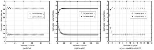As seen from Table 3, there is a considerable difference for the parameters $\stackrel{⁁}{\mathit{\xi }}$ estimated depending on whether the VCE methods is considered. The parameters based on the VCE are closer to the true values. Additionally, the MAE of estimation results by the VCE methods is also smaller in comparison to the methods of LS and TLS. Regarding the number of iterations, Scheme 4 has 38, while Scheme 3 and 5 have 43. Regarding the two proposed approaches, the convergence of Scheme 6 is relatively slow and the iteration number is 121. However, Scheme 7 requires only 20 iterations, which is more efficient. The convergence of the VCE for Schemes 3, 6 and 7 is given in Figure 2. According to the results of this example, the EM-VCE and the modified EM-NN-VCE accord with the three previous VCE methods.

Figure 1. Flowchart showing the implementation of the EM-VCE method for the partial EIV model.

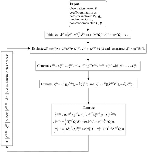
Figure 2. The convergence of the estimates of two variance factors ${\sigma }_1$ and ${\sigma }_2$ for the linear regression. (a) Variance factors ${\sigma }_1$ and ${\sigma }_2$ estimated by the REML method; (b) Variance factors ${\sigma }_1$ and ${\sigma }_2$ estimated by the EM-VCE method; and (c) Variance factors ${\sigma }_1$ and ${\sigma }_2$ estimated by the modified EM-NN-VCE method.

4.2. Planar coordinate transformation

To further demonstrate the validity of the proposed algorithms in the presence of negative variance, a planar coordinate transformation model is adopted as follows: (50) $$\left[\begin{array}{c}{X}_1\\ Y_1\\ ⋮\\ X_n\\ Y_n\end{array}\right]-\left[\begin{array}{c}{e}_{X_1}\\ e_{Y_1}\\ ⋮\\ e_{X_n}\\ e_{Y_n}\end{array}\right]=(\left[\begin{array}{cccc}{x}_1& -y_1& 1& 0\\ y_1& x_1& 0& 1\\ ⋮& ⋮& ⋮& ⋮\\ x_n& -y_n& 1& 0\\ y_n& x_n& 0& 1\end{array}\right]-\left[\begin{array}{cccc}{e}_{x_1}& e_{y_1}& 0& 0\\ e_{y_1}& e_{x_1}& 0& 0\\ ⋮& ⋮& ⋮& ⋮\\ e_{x_n}& e_{y_n}& 0& 0\\ e_{y_n}& e_{x_n}& 0& 0\end{array}\right])\left[\begin{array}{c}{\beta }_1\\ {\beta }_2\\ {\beta }_3\\ {\beta }_4\end{array}\right],$$(50)

where $(x_i,y_i)$ are the coordinates of the start coordinate system, $(X_i,Y_i)$ are the coordinates of the target coordinate system. $e_{x_i},$ $e_{y_i},$ $e_{X_i}$ and $e_{Y_i}$ are the errors of the corresponding coordinates. Subscripts $i$ expresses the $i\text{th}$ coordinates, and ${\beta }_1,$ ${\beta }_2,$ ${\beta }_3$ and ${\beta }_4$ are the coordinate transformation parameters.

Considering the planar coordinate transformation for the partial EIV model, the vector $\mathit{h}$ and the fixed matrix $\mathit{B}$ associated with the coefficient matrix are (51) $$\mathit{h}=\left[\begin{array}{c}{\mathit{h}}_1\\ {\mathit{h}}_2\\ {\mathit{h}}_3\\ {\mathit{h}}_4\end{array}\right],\mathit{B}=\left[\begin{array}{c}{\mathit{B}}_1\\ {\mathit{B}}_2\\ {\mathit{B}}_3\\ {\mathit{B}}_4\end{array}\right],$$(51)

where ${\mathit{h}}_1$ and ${\mathit{h}}_2$ are the $2n\times 1$ zero matrices, ${\mathit{h}}_3={\mathit{1}}_{n\times 1}\otimes \left[\begin{array}{c}1\\ 0\end{array}\right],$ ${\mathit{h}}_4={\mathit{1}}_{n\times 1}\otimes \left[\begin{array}{c}0\\ 1\end{array}\right],$ ${\mathit{B}}_1={\mathit{I}}_n\otimes \left[\begin{array}{cc}1& 0\\ 0& 1\end{array}\right],$ ${\mathit{B}}_2={\mathit{I}}_n\otimes \left[\begin{array}{cc}0& -1\\ 1& 0\end{array}\right]$ and ${\mathit{B}}_3={\mathit{B}}_4={\mathit{I}}_n\otimes \left[\begin{array}{cc}0& 0\\ 0& 0\end{array}\right].$

Given 15 sets of true values of the start coordinate system and 4 transformation parameters, the true coordinates of the target coordinate system are obtained from connecting two sets of coordinate systems. Then, we add random errors with a mean of $\mathit{0}$ and the covariance matrices of $1.5{\mathit{P}}_a^{-1}$ and $0.5{\mathit{P}}_y^{-1}$ to the two coordinate systems. A set of coordinates containing errors is listed in Table 4.

Table 4. Coordinate simulation values of two sets of coordinate systems.

Point	Start coordinate system		Target coordinate system
	$x_i$	$y_i$	$X_i$	$Y_i$
1	11.8943	13.2816	10.1465	33.6915
2	11.7518	24.4887	4.8716	43.0929
3	15.6519	17.0653	13.2569	39.2321
4	10.6345	15.3014	10.1712	34.0255
5	8.6522	10.9870	11.4955	30.5142
6	14.1360	18.6791	11.9610	41.0677
7	7.7877	11.9244	9.4339	30.3398
8	11.6892	10.9012	13.9029	32.1638
9	14.4061	19.1353	11.4364	41.2830
10	12.0893	14.8367	11.2776	34.3844
11	7.4895	15.3732	8.3223	33.8435
12	10.5787	20.3443	6.5422	39.9776
13	5.8489	22.9756	1.0869	38.2416
14	13.6018	15.5938	13.7017	37.4926
15	9.1771	24.4648	3.4518	42.5450

Assuming that the true values of the transformation parameters are $\mathit{\beta }={\left[\begin{array}{cccc}0.9& 0.6& 10& 15\end{array}\right]}^{{\rm T}},$ the weights of two sets of coordinate systems are as follows $$P_a=\mathit{\text{diag}}([1\mathrm{\hspace{0.17em}}\mathrm{\hspace{0.17em}}1\mathrm{\hspace{0.17em}}\mathrm{\hspace{0.17em}}1\mathrm{\hspace{0.17em}}\mathrm{\hspace{0.17em}}3\mathrm{\hspace{0.17em}}\mathrm{\hspace{0.17em}}3\mathrm{\hspace{0.17em}}\mathrm{\hspace{0.17em}}3\mathrm{\hspace{0.17em}}\mathrm{\hspace{0.17em}}2\mathrm{\hspace{0.17em}}\mathrm{\hspace{0.17em}}2\mathrm{\hspace{0.17em}}\mathrm{\hspace{0.17em}}2\mathrm{\hspace{0.17em}}\mathrm{\hspace{0.17em}}4\mathrm{\hspace{0.17em}}\mathrm{\hspace{0.17em}}4\mathrm{\hspace{0.17em}}\mathrm{\hspace{0.17em}}4\mathrm{\hspace{0.17em}}\mathrm{\hspace{0.17em}}6\mathrm{\hspace{0.17em}}\mathrm{\hspace{0.17em}}6\mathrm{\hspace{0.17em}}\mathrm{\hspace{0.17em}}6\mathrm{\hspace{0.17em}}\mathrm{\hspace{0.17em}}5\mathrm{\hspace{0.17em}}\mathrm{\hspace{0.17em}}5\mathrm{\hspace{0.17em}}\mathrm{\hspace{0.17em}}5\mathrm{\hspace{0.17em}}\mathrm{\hspace{0.17em}}7\mathrm{\hspace{0.17em}}\mathrm{\hspace{0.17em}}7\mathrm{\hspace{0.17em}}\mathrm{\hspace{0.17em}}7\mathrm{\hspace{0.17em}}\mathrm{\hspace{0.17em}}9\mathrm{\hspace{0.17em}}\mathrm{\hspace{0.17em}}9\mathrm{\hspace{0.17em}}\mathrm{\hspace{0.17em}}9\mathrm{\hspace{0.17em}}\mathrm{\hspace{0.17em}}8\mathrm{\hspace{0.17em}}\mathrm{\hspace{0.17em}}8\mathrm{\hspace{0.17em}}\mathrm{\hspace{0.17em}}8\mathrm{\hspace{0.17em}}\mathrm{\hspace{0.17em}}12\mathrm{\hspace{0.17em}}\mathrm{\hspace{0.17em}}12\mathrm{\hspace{0.17em}}\mathrm{\hspace{0.17em}}12]),$$ $$P_y=\mathit{\text{diag}}([11\mathrm{\hspace{0.17em}}\mathrm{\hspace{0.17em}}11\mathrm{\hspace{0.17em}}\mathrm{\hspace{0.17em}}11\mathrm{\hspace{0.17em}}\mathrm{\hspace{0.17em}}8\mathrm{\hspace{0.17em}}\mathrm{\hspace{0.17em}}8\mathrm{\hspace{0.17em}}\mathrm{\hspace{0.17em}}8\mathrm{\hspace{0.17em}}\mathrm{\hspace{0.17em}}10\mathrm{\hspace{0.17em}}\mathrm{\hspace{0.17em}}10\mathrm{\hspace{0.17em}}\mathrm{\hspace{0.17em}}10\mathrm{\hspace{0.17em}}\mathrm{\hspace{0.17em}}7\mathrm{\hspace{0.17em}}\mathrm{\hspace{0.17em}}7\mathrm{\hspace{0.17em}}\mathrm{\hspace{0.17em}}7\mathrm{\hspace{0.17em}}\mathrm{\hspace{0.17em}}6\mathrm{\hspace{0.17em}}\mathrm{\hspace{0.17em}}6\mathrm{\hspace{0.17em}}\mathrm{\hspace{0.17em}}6\mathrm{\hspace{0.17em}}\mathrm{\hspace{0.17em}}4\mathrm{\hspace{0.17em}}\mathrm{\hspace{0.17em}}4\mathrm{\hspace{0.17em}}\mathrm{\hspace{0.17em}}4\mathrm{\hspace{0.17em}}\mathrm{\hspace{0.17em}}5\mathrm{\hspace{0.17em}}\mathrm{\hspace{0.17em}}5\mathrm{\hspace{0.17em}}\mathrm{\hspace{0.17em}}5\mathrm{\hspace{0.17em}}\mathrm{\hspace{0.17em}}2\mathrm{\hspace{0.17em}}\mathrm{\hspace{0.17em}}2\mathrm{\hspace{0.17em}}\mathrm{\hspace{0.17em}}2\mathrm{\hspace{0.17em}}\mathrm{\hspace{0.17em}}3\mathrm{\hspace{0.17em}}\mathrm{\hspace{0.17em}}3\mathrm{\hspace{0.17em}}\mathrm{\hspace{0.17em}}3\mathrm{\hspace{0.17em}}\mathrm{\hspace{0.17em}}1\mathrm{\hspace{0.17em}}\mathrm{\hspace{0.17em}}1\mathrm{\hspace{0.17em}}\mathrm{\hspace{0.17em}}1]).$$

In Table 5, a negative variance component appears by Scheme 3. Scheme 5 imposes non-negativity constraints based on the LS-VCE theory, the variance factors are non-negative. Scheme 4 fails to converge due to its improper stochastic model. Also, Scheme 3 lacks good estimation results in Table 5, the MAE is even worse than the LS and TLS. The MAE of estimation results by the non-negative VCE methods is negligible due to a small amplitude of the variance component obtained. In this article, the convergence threshold of Scheme 5 is set as $\epsilon ={10}^{-10},$ the variance components are close to those of Schemes 5 and 7. The convergence of the variance components of Schemes 3, 5 and 7 is shown in Figure 3. Nineteen iterations are needed for the REML. However, only 10 and 11 iterations are required for the NNLS-VCE and the modified EM-NN-VCE, respectively.

Figure 3. The convergence of the estimates of two variance factors ${\sigma }_1$ (left column) and ${\sigma }_2$ (right column) for the coordinate transformation. (a) Variance factor ${\sigma }_1$ estimated by the REML method; (b) Variance factor ${\sigma }_2$ estimated by the REML method; (c) Variance factor ${\sigma }_1$ estimated by the NNLS-VCE method; (d) Variance factor ${\sigma }_2$ estimated by the NNLS-VCE method; (e) Variance factor ${\sigma }_1$ estimated by the modified EM-NN-VCE method; and (f) Variance factor ${\sigma }_2$ estimated by the modified EM-NN-VCE method.

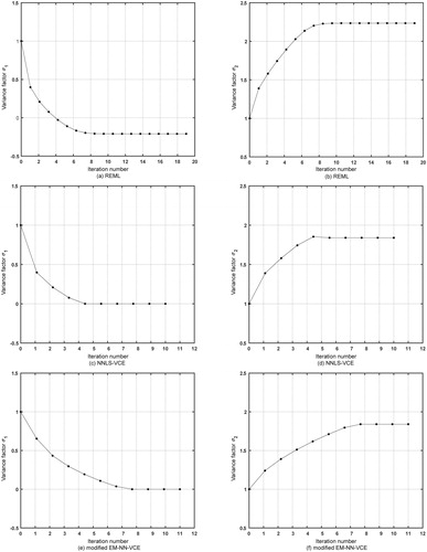
Table 5. Coordinate transformation results with different methods.

VCE	Scheme 1	Scheme 2	Scheme 3	Scheme 4	Scheme 5	Scheme 6	Scheme 7
${\widehat{\sigma }}_1$	–	–	–0.209447	–	0.000000	0.000025	0.000000
${\widehat{\sigma }}_2$	–	–	2.235087	–	1.839956	1.839925	1.839956
MAE	0.611943	0.172041	0.698922	–	1.2385e–13	4.9938e–8	1.2385e–13

In Table 6, different convergence thresholds are set for Scheme 6. As the threshold decreases, both variance components converge to a certain trend value. The variance factor ${\widehat{\sigma }}_1$ estimated approaches zero. The variance factor ${\widehat{\sigma }}_2$ also converges to a positive value. This approach guarantees the non-negativity of the variance components. In fact, when the variance factor ${\widehat{\sigma }}_1$ approaches zero, the likelihood function $l_M(\mathit{\theta };{\mathit{y}}_c)$ of the complete data ${\mathit{y}}_c$ will approach infinity. In that case, the variance component estimated by EM-VCE tend to converge slowly, maximizing the likelihood function is actually an ill-posed problem. Thereby, an approximate value with zero for variance component is feasible, the EM-VCE could be applied to verify the justification of the existing non-negative VCE methods.

Table 6. Results of Scheme 6 with different convergence thresholds.

VCE	10^–6	10^–7	10^–8	10^–9	10^–10	10^–11	10^–12
${\widehat{\sigma }}_1$	0.002467	0.000778	0.000246	0.000078	0.000025	0.000007	0.000003
${\widehat{\sigma }}_2$	1.836872	1.838982	1.839648	1.839859	1.839925	1.839946	1.839953

5. Conclusions

In some geodetic applications, the problem of negative variances may appear in the process of correcting the stochastic model with variance factors. Many attempts have been made to counteract this effect, such as PVFs-VCE and NNLS-VCE, this problem may be avoided by introducing the positive-valued functions or non-negativity constraints. To investigate the properties of solutions from the statistics, an unconstrained approach is required. Based on the standard theories of the EM algorithm, we develop two new methods of non-negative VCE for the partial EIV model, an iterative algorithm of TLS is obtained simultaneously. The EM-VCE can statistically demonstrate that the problem of maximum likelihood estimation is essentially an ill-posed problem in the presence of negative estimates and variance component estimates move to the edge of the parameter space. A modified version of VCE is also presented to improve the computational efficiency and has access to the non-negative estimates. Both algorithms are free from a complex matrix inversion. Finally, two numerical examples, i.e. linear regression and the four-parameter planar coordinate transformation, are employed to verify the feasibility of the proposed algorithms. The results of linear regression show that the proposed algorithms can achieve the more reasonable fixed parameter estimates compared with the algorithms of LS and TLS. The variance component estimates are identical to the algorithms of REML, PVFs-VCE and NNLS-VCE, the modified EM algorithm, namely, EM-NN-VCE, which is nearly fifty percent faster. Two variance factors of the latter example were simultaneously estimated to be non-negative by the proposed algorithms. This study provides a statistical explanation for the justifiability of the existing non-negative VCE methods.

Disclosure statement

No potential conflict of interest was reported by the authors.

Additional information

Funding

This research is supported by the National Natural Science Foundation of China (Nos. 41874001 and 41664001); Support Program for Outstanding Youth Talents in Jiangxi Province (No. 20162BCB23050); National Key Research and Development Program (No. 2016YFB0501405).

References

- Amiri-Simkooei AR. 2013. Application of least squares variance component estimation to errors-in-variables models. J Geod. 87(10–12):935–944.
- Amiri-Simkooei AR. 2016. Non-negative least-squares variance component estimation with application to GPS time series. J Geod. 90(5):451–466.
- Amiri-Simkooei AR, Jazaeri S. 2012. Weighted total least squares formulated by standard least squares theory. J Geod Sci. 2(2):113–124.
- Calvin JA. 1993. REML estimation in unbalanced multivariate variance components models using an EM algorithm. Biometrics. 49(3):691–701.
- Dempster AP, Laird NM, Rubin DB. 1977. Maximum likelihood from incomplete data via the EM algorithm. J R Stat Soc Ser B. 39(1):1–38.
- Diffey SM, Smith AB, Welsh AH, Cullis BR. 2017. A new REML (parameter expanded) EM algorithm for linear mixed models. Aust N Z J Stat. 59(4):433–448.
- El Leithy HA, Abdel Wahed ZA, Abdallah MS. 2016. On non-negative estimation of variance components in mixed linear models. J Adv Res. 7(1):59–68.
- Fang X. 2011. Weighted total least squares solutions for applications in geodesy. Hanover, Germany: Leibniz Universität Hannover.
- Fang X. 2013. Weighted total least squares: necessary and sufficient conditions, fixed and random parameters. J Geod. 87(8):733–749.
- Fang X, Li B, Alkhatib H, Zeng W, Yao Y. 2017. Bayesian inference for the errors-in-variables model. Stud Geophys Geod. 61(1):35–52.
- Foulley JL, Jaffrézic F, Robert-Granié C. 2000. EM-REML estimation of covariance parameters in Gaussian mixed models for longitudinal data analysis. Genet Sel Evol. 32(2):129–141.
- Franc V, Hlaváč V, Navara M. 2005. Sequential coordinate-wise algorithm for the non-negative least squares problem. In: Gagalowicz A, Philips W (eds) Computer analysis of images and patterns, Lecture Notes in Computer Science. p. 407–414.
- Golub GH, Van Loan CF. 1980. An analysis of the total least squares problem. SIAM J Numer Anal. 17(6):883–893.
- Grafarend EW, Schaffrin B. 1993. Ausgleichungsrechnung in linearen modellen. Mannheim, Germany: BI-Wissenschaftsverlag.
- Groeneveld E. 1994. A reparameterization to improve numerical optimization in multivariate REML (co)variance component estimation. Genet Sel Evol. 26(6): 537–545.
- Gupta MR, Chen Y. 2010. Theory and use of the EM algorithm. FNT Signal Process. 4(3):223–296.
- Helmert FR. 1907. Die Ausgleichungsrechnung nach der Methode der kleinsten Quadrate. Berlin, Germany: Zweite Auflage, Teubner, Leipzig.
- Hsu R. 1999. An alternative expression for the variance factors in using iterated almost unbiased estimation. J Geod. 73(4):173–179.
- Jazaeri S, Amiri-Simkooei AR, Sharifi MA. 2014. Iterative algorithm for weighted total least squares adjustment. Surv Rev. 46(334):19–27.
- Jennrich RI, Sampson PF. 1976. Newton-Raphson and related algorithms for maximum likelihood variance component estimation. Technometrics. 18(1):11–17.
- Kargoll B, Omidalizarandi M, Loth I, Paffenholz J-A, Alkhatib H. 2018. An iteratively reweighted least-squares approach to adaptive robust adjustment of parameters in linear regression models with autoregressive and t-distributed deviations. J Geod. 92(3):271–297.
- Koch KR. 1986. Maximum likelihood estimate of variance components. Bull Geod. 60(4):329–338.
- Koch KR. 1999. Parameter estimation and hypothesis testing in linear models. Berlin, Germany: Springer-Verlag.
- Koch KR. 2013. Robust estimation by expectation maximization algorithm. J Geod. 87(2):107–116.
- Koch KR, Kargoll B. 2013. Expectation maximization algorithm for the variance-inflation model by applying the t-distribution. J Appl Geod. 7(3):217–225.
- Laird NM, Ware JH. 1982. Random-effects models for longitudinal data. Biometrics. 38(4):963–974.
- Lange KL, Little RJA, Taylor JMG. 1989. Robust statistical modeling using the t distribution. J Am Stat Assoc. 84(408):881–896.
- Lee J, Khuri AI. 2001. Modeling the probability of a negative ANOVA estimate of a variance component. CSAB. 51(1–2):31–45.
- Little RJA, Rubin DB. 2002. Statistical analysis with missing data. 2nd ed. Hoboken (NJ): Wiley.
- Liu JN, Zeng WX, Xu PL. 2013. Overview of total least squares methods. Geom Inform Sci. 38(5):505–512.
- Mclachlan GJ, Krishnan T. 2008. The EM algorithm and extensions. 2nd ed. Hoboken (NJ): Wiley.
- Moghtased-Azar K, Tehranchi R, Amiri-Simkooei AR. 2014. An alternative method for non-negative estimation of variance components. J Geod. 88(5):427–439.
- Peng J. 2009. Jointly robust estimation of unknown parameters and variance components based on expectation-maximization algorithm. J Surv Eng. 135(1):1–9.
- Schaffrin B, Wieser A. 2008. On weighted total least-squares adjustment for linear regression. J Geod. 82(7):415–421.
- Searle SR, Casella G, McCulloch CE. 1992. Variance components. New York (NY): Wiley.
- Sjöberg LE. 2011. On the best quadratic minimum bias non-negative estimator of a two-variance component model. J Geod Sci. 1(3):280–285.
- Sun Y, Sinha BK, Rosen DV, Meng Q. 2003. Nonnegative estimation of variance components in multivariate unbalanced mixed linear models with two variance components. J Stat Plan Infer. 115(1):215–234.
- Teunissen PJG, Amiri-Simkooei AR. 2008. Least-squares variance component estimation. J Geod. 82(2):65–82.
- Thompson WA, Jr. 1962. The problem of negative estimates of variance components. Ann Math Statist. 33(1):273–289.
- Vergos GS, Tziavos IN, Sideris MG. 2012. On the determination of sea level changes by combining altimetric, tide gauge, satellite gravity and atmospheric observations. Heidelberg, Berlin: Springer.
- Wang L. 2012. Properties of the total least squares estimation. Geod Geodyn. 3(4):39–46.
- Wang L, Ding R. 2020. Inversion and precision estimation of earthquake fault parameters based on scaled unscented transformation and hybrid PSO/Simplex algorithm with GPS measurement data. Measurement. 153:107422.
- Wang L, Wen G, Zhao Y. 2019. Virtual observation method and precision estimation for ill-posed partial EIV model. J Surv Eng. 145(4):04019010.
- Wang L, Xu G. 2016. Variance component estimation for partial errors-in-variables models. Stud Geophys Geod. 60(1):35–55.
- Wang L, Yu H, Chen X. 2016. An algorithm for partial EIV model. Acta Geod Cartographica Sin. 45(1):22–29.
- Wang L, Zhao Y. 2018. Scaled unscented transformation for nonlinear error propagation:accuracy, sensitivity and applications. J Surv Eng. 144(1):04017022.
- Wang L, Zhao Y. 2019. Second order approximating function method for precision estimation of total least squares. J Surv Eng. 145(1):04018011.
- Wang L, Zou C. 2019. Accuracy analysis and applications of Sterling interpolation method for nonlinear function error propagation. Measurement. 146:55–64.
- Xu P, Liu Y, Shen Y, Fukuda Y. 2007. Estimability analysis of variance and covariance components. J Geod. 81(9):593–602.
- Xu P, Liu J, Shi C. 2012. Total least squares adjustment in partial errors-in-variables models: algorithm and statistical analysis. J Geod. 86(8):661–675.
- Xu P, Shen Y, Fukuda Y, Liu Y. 2006. Variance component estimation in linear inverse ill-posed models. J Geod. 80(2):69–81.
- Zhao J, Guo F, Li Q. 2019. Fisher-Score algorithm of WTLS estimation for PEIV model. Geom Inform Sci Wuhan Univ. 44(2):59–65.
- Zhou H, Hu L, Zhou J, Lange K. 2015. MM algorithms for variance components models. J Comput Graph Stat. arXiv: 1509. 07426.