Flood susceptibility mapping using an improved analytic network process with statistical models

Abstract

Flooding is a natural disaster that causes considerable damage to different sectors and severely affects economic and social activities. The city of Saqqez in Iran is susceptible to flooding due to its specific environmental characteristics. Therefore, susceptibility and vulnerability mapping are essential for comprehensive management to reduce the harmful effects of flooding. The primary purpose of this study is to combine the Analytic Network Process (ANP) decision-making method and the statistical models of Frequency Ratio (FR), Evidential Belief Function (EBF), and Ordered Weight Average (OWA) for flood susceptibility mapping in Saqqez City in Kurdistan Province, Iran. The frequency ratio method was used instead of expert opinions to weight the criteria in the ANP. The ten factors influencing flood susceptibility in the study area are slope, rainfall, slope length, topographic wetness index, slope aspect, altitude, curvature, distance from river, geology, and land use/land cover. We identified 42 flood points in the area, 70% of which was used for modelling, and the remaining 30% was used to validate the models. The Receiver Operating Characteristic (ROC) curve was used to evaluate the results. The area under the curve obtained from the ROC curve indicates a superior performance of the ANP and EBF hybrid model (ANP-EBF) with 95.1% efficiency compared to the combination of ANP and FR (ANP-FR) with 91% and ANP and OWA (ANP-OWA) with 89.6% efficiency.

Keywords:

• Flood mapping
• analytic network process (ANP)
• statistical models
• Saqqez City

1. Introduction

The rapid increase in urbanization and the effects of climate change have led to numerous environmental problems and disasters in recent years (Rahmati et al. 2019; Malik et al. 2020b). Floods are one of the most destructive natural disasters (Doocy et al. 2013), causing significant loss of life worldwide and financial damage that equates to 40% of the total economic loss caused by all-natural disasters annually (Janizadeh et al. 2019). Any type of land-use change resulting from urbanization leads to an increase in flooding due to the rise in the rainfall-runoff coefficient (Myronidis et al. 2016; Dammalage and Jayasinghe 2019). Preventing floods is complicated, but their occurrence can be predicted and partially controlled using appropriate methods and measures (Mansur et al. 2018; Malik and Pal 2020). Having access to accurate and current information is key to preventing floods or at least reducing their harmful effects. One of these key pieces of information is a flood potential map (Papaioannou et al. 2018). Morphological changes caused by human activities can have a significant impact on changing the conditions for floods (Yousefi et al. 2018).

So that, urbanization, deforestation, and the impact of climate change on rainfall characteristics in susceptible areas may all contribute to an increase in flooding (Kundzewicz et al. 2014). Many factors are important in determining flood risk zones, the most important of which are land use/land cover, geology, slope, drainage network and morph metric factors in general (Rahmati et al. 2019). Also, the river network in an area can be one of the most effective reasons for the morphological change of floods, and this morphological change will be caused by human interaction and communication with the rivers (Yousefi et al. 2019).

Present flood control measures have failed to mitigate flood problems. It is not possible to eliminate the flood problems, but with proper flood forecasting system and management, damages can be minimized (Das et al. 2018, 2019). Flood zoning provides valuable information regarding the nature of the floods, their effects on the floodplain, and determining the riparian zone (Roopnarine et al. 2018). GIS is a useful tool for investigating multidimensional events, such as floods, at various spatial and temporal scales. Spatial analysis with GIS has been used to determine flood zones (Chowdhuri et al. 2020). Also, the use of remote sensing data, along with improved modelling techniques, such as data mining and machine learning, could help to determine flood-prone areas better.

Several variables affect the occurrence of floods in a watershed and determining the flood catchment areas is an important factor in investigating the floodplains. The most important factors and variables are physical and natural factors (e.g. elevation, slope, aspect, slope curvature, lithology, topographic position index and rainfall), hydrological factors (e.g. drainage density, river distance, topographic wetness index, and stream power index) and human disturbance factors (e.g. land use and road distance) (Al-Juaidi et al. 2018; Zhao et al. 2018; Darabi et al. 2019; Costache 2019a). Recently, several methods and models have been used to study flood hazards. The wildly applied methods and models for flood hazard mapping are Logistic Regression (LR) (Hong et al. 2018; Lee et al. 2018; Rahmati et al. 2019; Malik et al. 2020a), Weights of Evidence (WofE) (Hong et al. 2018), Support Vector Machine (SVM) (Hong et al. 2018; Tavakkoli Piralilou et al. 2019; Ghorbanzadeh et al. 2019c), Random Forest (RF) (Avand et al. 2019; Chen et al. 2019; Darabi et al. 2019; Shahabi et al. 2019), Frequency Ratio (FR) (Lee et al. 2018; Rahman et al. 2019), Decision Tree (DT) (Chen et al. 2019) and Naïve Bayes Tree (NBT) (Khosravi et al. 2019). In addition to these models, multi-criteria decision-making techniques such as the analytic hierarchy process (AHP) (Satty 1980) and the Analytic Network Process (ANP), which is an extended version of the AHP and consider as a more appropriate approach for complex decision problems can also be used for flood hazard mapping (Ahmadlou et al. 2019; Kanani-Sadat et al. 2019). Although these models have criticized for their some inabilities and associated uncertainties, they have optimized by integrating with several statistical and mathematical techniques (Ghorbanzadeh et al. 2019b). The statistical techniques of the sensitivity and uncertainty analyses have been applied along with the AHP and ANP by using the Monte Carlo simulation (MCS) (Ghorbanzadeh et al. 2018b, 2019a). The frequency ratio (FR) also has combined with the AHP in the hybrid spatial multi-criteria evaluation (SMCE) method to enhance the overall accuracy of criteria weightings. Moreover, Ha et al. (2017) applied the AHP, which was integrated with fuzzy-TOPSIS for their study. The fuzzy logic has been integrated with both the AHP and ANP to evolve their results in a number of studies to minimize the uncertainty associated with decision-making procedure. Ghorbanzadeh et al. (2018a) applied the interval matrices for pairwise comparisons of AHP, which could be helpful for the cases that a lot of experts with a high variation of preferences are involved in complex decisions. The combination of GIS and multi-criteria decision-making has already been used in spatial modelling and disaster analysis of natural disasters such as floods (Paquette and Lowry 2012; Solín 2012; Kazakis et al. 2015). The primary purpose of this research is flood susceptibility mapping using improved ANP with statistical models. Moreover, we evaluated the efficiency of the FR, EBF and OWA methods in providing flood probability and susceptibility maps for Saqqez City in north-west Iran.

2. Materials and methods

2.1. Description of the study area

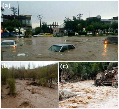
The study area is Saqqez City, which is located in the Zagros mountains in the north of Kurdistan Province (51° 45° 46° 51° east longitude and 35° 46° 36° 36° north latitude) (Figure 1(b)). The city has an area of about 4514 km² and a population of 226.451(2016 Census). The average annual rainfall in the study area is 450 mm. Rainfall usually starts in the springtime, and during June, July, and August the city is at risk of flooding. There are many streams and also many springs which underlie the genesis of the rivers located across the study area. The notable rivers of the study area are Zarinehrood, Khorkhor, and Saqqez (Figure 1(c)). Due to a lack of flood control measures and improper flood management, the leading causes of flooding in the urban and rural areas are the rivers (Figure 2).

Figure 1. Study area: (a) location of Kurdistan in Iran, (b) Saqqez in Kurdistan, and (c) Saqqez Catchment.

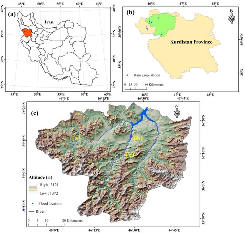
Figure 2. The location of the flooding points in the study area.

2.2. Methodology

2.2.1. Proposed process

Flood susceptibility mapping (FSM) in this study was performed with a new approach, by combining the ANP multi-criteria decision model with FR, EBF, and OWA statistical models in five stages (Figure 3).

Figure 3. Flowchart of the methodology for flood susceptibility modelling.

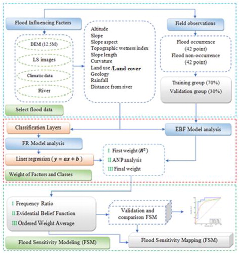
• Collecting data and information from the study area to prepare a map related to Flood Conditional Factors (FCFs) and a flood inventory map.

• Multi-collinearity test was performed to ensure the independent effect of each FCFs.

• Determining the relationship between the locations of occurring floods and FCFs classes using Frequency Ratio (FR) and Evidential Belief Function (EBF) algorithms.

• Using a linear regression relationship and FR values for each class of factors, the initial weight values for FCFs were calculated.

• The importance (final weight) of each of the factors used in this study was determined using the initial weights in the Analytic Network Process (ANP) model.

• The calculated values of FR and belief (Bel) were applied to each of the sensitivity classes in each factor.

• For Flood susceptibility modelling, new combined models ANP-FR, ANP-EBF, and ANP-OWA were made by applying secondary weight to each of the factors.

• The performance of flood forecasting models was evaluated using Receiver Operating Characteristic (ROC) curve and area under the curve (AUC), standard error (SE) and confidence interval (CI) values.

2.2.2. Flood inventory map (FIM)

A flood distribution map is one of the most critical layers in flood susceptibility mapping, which is based on the analyzes of correlations between factors affecting the flood and the location of the flood (flood zones) in the region (Das et al. 2018). Also, considering that in the study area, the conditions of floods (geographical, climatic, etc.) have not changed much compared to previous years; previous flood points can be used to predict future flood zones. In total, 42 flood events have been recorded in the Saqqez Catchment using the flood line and field investigation. The data regarding flood locations were extracted from the archive of the Water Resources Management Organization which provided the flood locations as points. It should be mentioned that this institution is the official authority in Iran in the domain of hydrology and water management. The use of flood locations as points is also recommended by the high-quality results and models performances higher than 90%, that were achieved in the previous studies related to the flood susceptibility assessment (Chapi et al. 2017; Choubin et al. 2019; Bui et al. 2019a; Ali et al. 2020; Yariyan et al. 2020c). Also, after obtaining data about the flood locations, using field research and regional documents, the occurrence of floods in each place was ensured. We used 70% of these flood location points to map potential flooding and the remaining 30% to validate the models (Costache 2019b).

2.2.3. Flood conditional factors (FCFs)

Determining the factors affecting flooding is one of the essential steps in mapping flood potential (Pham et al. 2016). In this study, the 10 factors influencing floods are slope, slope aspect, curvature, altitude, rainfall, distance from river, topographic wetness index, slope length, lithology and land use/land cover (LU/LC). By collecting information about 10 factors affecting the flood, all maps with a pixel size of 90 × 90 and a scale of 1: 600,000 were converted to raster format. Each factor was divided into several classes (Figure 4). The map classification related to each of the factors was done by the Natural break method to perform FR analysis and better display. ArcGIS and SAGA GIS software was used to provide the required layers by using a digital elevation model (DEM) with a spatial resolution of 12.5 meters. The DEM was downloaded from the ALOSPALSAR sensor from Landsat images. When high-precision topographic data are used, flood analysis has good predictive accuracy . Therefore, the elevation layer and its derivatives have a significant impact on the prediction of flood-prone areas. The altitude class map is based on the digital elevation model and comprises 5 classes (Figure 4(f)) (Bui et al. 2019b). The slope is the most critical factor for flooding due to its direct influence on surface runoff in watersheds. The effect of slope on the occurrence of devastating floods is related to runoff speed (Yariyan et al. 2020c). So that, on slopes with high slopes, the speed of water penetration is much lower, this will increase the speed and flow of water. The slope map of the study area is based on the digital elevation model and is classified into 5 classes (Figure 4(a)) (Khosravi et al. 2019). Earth curvature is another factor related to flooding. The earth curvature layer is also based on the digital elevation model and comprises three classes; concave (positive values (+)), convex (negative values (-)), and flat (value 0) (Figure 4(g)) (Youssef et al. 2016). The slope aspect is a further factor influencing flooding. This map in 9 class (flat, northeast, east, southeast, south, southwest, west, and northwest) was created using the digital elevation model (Figure 4(e)) (Bathrellos et al. 2018).

Figure 4. Maps of flood-influencing factors: (a) Slope, (b) Rainfall, (c) Sloe length, (d) Topographic wetness index, (e) Aspect, (f) Altitude, (g) Curvature, (h) Distance from river, (i) Geology, and (j) Land use/Land cover.

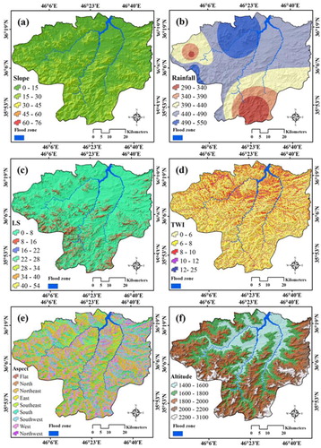
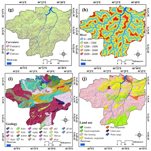
The slope length layer produced by the combination of the catchment area and the slope layers affects the water flow. We used this layer to examine the influence of the topography on the flood flow. The topographic wetness index (TWI) is used to measure topographic control in hydrological studies (Chen and Yu 2011). The TWI factor indicates the amount of cumulative flow associated with a point in the watershed that tends to move to less sloping areas under the influence of gravity (Janizadeh et al. 2019). Therefore, it cans gravity to increase water flow velocity and destructive power. Also, the amount of spatial distribution for runoff production will be identified by measuring TWI. Therefore, the TWI parameter related to water flow can be calculated through the following equation: (1) $$\mathrm{TWI}=\ln \left(\frac{A_s}{\beta }\right)\mathrm{ }$$(1) where$A_s$ is the catchment area and $\beta$ is the slope (in degrees). The TWI and slope length (SL) were prepared using SAGA GIS software version 3.2 (Figure 4(c,d)).

The rainfall layer was developed based on the collected data from seven rain gauge stations (Figure 1(b)) Baneh, Boein, Bastam, Kelahshin, Vezmaleh, Miradeh, and Saqqez for the period 1999–2018. The rainfall map in five classes from 290 to 550 mm have been classified and prepared by the data of the Meteorological Organization of Iran (Figure 4(b)). We used the inverse distance weighted (IDW) method in GIS to interpolate the precipitation stations in the study area. Distance from the river is an important and influential factor in reducing or intensifying the occurrence of floods (Khosravi et al. 2018) because the areas adjacent to the river are more prone to floods. In this study, the river network was extracted using the ‘Arc hydro’ integration tool in ArcGIS through DEM, and then a layer of distance from river was prepared using the ‘Euclidean distance’ tool (Figure 4(h)). Land use/Land cover plays an essential role in the flooding process and directly or indirectly affects some hydrological processes such as permeability, evapotranspiration, and runoff (Hölting and Coldewey 2019). When it rains in a basin, the amount of rain that enters the rivers depends on the conditions of the area, topography, and LU/LC. The land use/land cover map of the study area was prepared using the Landsat Eight image and OLI sensor on 2018.06.20. The generated LU/LC map has 7 classes, namely: garden, good rangelands, dry farming, moderate rangelands, poor rangelands, urban area, and water (Figure 4(j)). The geology of the area plays a key role in mapping the potential of floods because many geological units are active in hydrological processes, also can have a great impact on the conduction and penetration of water flow. The geological layer was prepared using a 1:100000 map of Kurdistan Province and include 26 geological units (Figure 4(i); Table 1).

Table 1. The Geology of the Saqqez area.

Row	Geology	Code	Area (%)	Permeability classes
1	Dark red moderate—grained arkosic	Cl	0.36	Low
2	Nummulitic limestone	E2l	0.46	High
3	Tuff, volcanic rock	Ek	0.56	High
4	Cretaceous rocks in general	K	14.99	High
5	Andesitic volcanic	K2av	0.60	High
6	Andesitic volcanic	Kav	11.81	High
7	Dark grey argillaceous shale	Kfsh	0.20	Moderate
8	Marl, shale, sandy limestone and sandy dolomite	Klsm	14.31	High
9	Grey thick—bedded to massive orbitolina limestone	Klsol	0.04	Moderate
10	Upper cretaceous, undifferentiated rocks	Ku	2.73	Low
11	Massive to thick—bedded reefal limestone	OMql	2.09	Moderate
12	Granite	Ogr	5.98	Low
13	Granite	PAgr	2.89	Low
14	Marl, shale, sandstone and conglomerate	Plms	1.74	High
15	Dark grey moderate—massive limestone	Pr	32.32	High
16	Undifferentiated lower Paleozoic rocks	Pz	0.35	Low
17	Old terraces	Qft1	0.02	Moderate
18	Younger gravel fans and terraces	Qft2	3.13	High
19	Dark grey shale and sandstone	TRJs	1.45	High
20	Marble	mb	2.49	Low
21	Thick dolomite and limestone unit	pC-Cs	1.22	Low
22	Granite gneiss and locally including migmatite	pCgn	0.27	Low
23	Precambrian granite to granodiorite	pCgr	0.36	Low
24	Marble	pCmb	0.46	Low
25	Moderate—grade, regional metamorphic rocks	pCmt1	0.56	Low
26	Dolomite and limestone, partly cherty	pCr	14.99	Moderate

The information on formations in this area is shown in Table 1. The distance from the river map was prepared using GIS software and classified into 5 classes (Figure 4(h)).

2.3. Description of the models

2.3.1. Analytic network process (ANP) model

The purpose of decision-making is to choose the best option by weighing up the influencing factors. Multi-criteria decision-making methods use multi-criteria rather than an optimal measurement criterion (Ghorbanzadeh et al. 2018a; Mitroulis and Kitsios 2019). All elements must be well understood and precisely defined to model and analyze a multi-criteria system (Yariyan et al. 2019). The analytic network process is one of the multi-criteria decision-making techniques that fall into the category of compensatory models (Alilou et al. 2019). This model is designed based on the hierarchical analysis process, and the network has replaced the hierarchy (Peng and Tzeng 2019).

One of the assumptions of the hierarchical analysis process is that the higher sections and branches of the hierarchy are independent of the lower sections and branches (Saaty 2004). In many decisions, however, decision elements cannot be modelled hierarchically and independently of each other, therefore, different elements are combined. Saaty (2004) suggests using the ANP technique to this end. In the ANP, the relationships between different levels of decision-making are considered one-way. The advantage of the ANP approach is that the various elements are measured based on their inter-relationships (Ghorbanzadeh et al. 2018b). Unlike the AHP model, which uses an entirely hierarchical structure for modelling, the ANP model uses a pairwise comparative measurement scale and performs modelling using the system perspective feedback (Alizadeh et al. 2018).

In this ANP model, the initial value for each factor is determined on a scale of 1 to 9. After the pairwise comparisons matrix is formed, the local priority vector is calculated using the following formula: (2) $$A=\lambda \mathit{max}\mathrm{ }$$(2)

Where $A$ is the pairwise comparison matrix and $\lambda \mathit{max}$ is the largest value in this matrix, which is calculated as follows: (3) $$\lambda \mathit{max}=\sum _{j=1\mathrm{ }}^n\mathrm{ }[W_j\sum _{i=1}^m{a}_{ij}]\mathrm{ }$$(3) where $a_{ij}$ is the value of the factor and $W_j$ is its weight. The weights of any pairwise comparison matrix can be calculated separately. Moreover, the resulting weights are organized in an overall supermatrix for evaluating the final weights of criteria (Ghorbanzadeh et al. 2018b).

$\mathit{Wij}$ Component of Super matrix (4) $$W=\left[\begin{array}{cc}\begin{array}{c}{W_{i1}}^{\left(j1\right)}\\ {W_{i2}}^{\left(j1\right)}\\ \begin{array}{c}⋮\\ {W_{i{n}_i}}^{\left(j1\right)}\end{array}\end{array}& \begin{array}{c}{W_{i1}}^{\left(j2\right)}\\ {W_{i2}}^{\left(j2\right)}\\ \begin{array}{c}⋮\\ {W_{i{n}_i}}^{\left(j2\right)}\end{array}\end{array}\end{array}\begin{array}{cc}\begin{array}{c}\dots \\ \dots \\ \begin{array}{c}⋮\\ \dots \end{array}\end{array}& \begin{array}{c}{W_{i1}}^{\left(j{n}_j\right)}\\ {W_{i2}}^{\left(j{n}_j\right)}\\ \begin{array}{c}⋮\\ {W_{i{n}_i}}^{\left(j{n}_j\right)}\end{array}\end{array}\end{array}\right]\mathrm{ }$$(4)

The resulting values from the limited matrix are considered as the final relative weight $W = (w1, w2, .., wn)$ that is calculated using the supermatrix. The whole process of the limit matrix is fully explained by Saaty (2007).

After carrying out the ANP, the value of the CR compatibility index is calculated (Equation (5)(5) $$\mathrm{CR}=\frac{(\lambda \mathit{max}\mathrm{ }-\mathrm{ }n)\mathrm{ }}{\mathrm{ }(n\mathrm{ }-\mathrm{ }1)\mathrm{ }}/\mathrm{RI}\mathrm{ }$$(5) ). If its value is CR ≤ 0.1, the matrix is compatible. (5) $$\mathrm{CR}=\frac{(\lambda \mathit{max}\mathrm{ }-\mathrm{ }n)\mathrm{ }}{\mathrm{ }(n\mathrm{ }-\mathrm{ }1)\mathrm{ }}/\mathrm{RI}\mathrm{ }$$(5) where n is the rank of the arbitration matrix, and RI is a random index type with the following values (Alizadeh et al. 2018) (Table 2).

Table 2. Random consistency index (RI).

n	1	2	3	4	5	6	7	8	9	10	11	…
RI	0	0	0.58	0.90	1.12	1.24	1.32	1.41	1.45	1.49	1.51	…

2.3.2. Frequency ratio (FR)

The frequency ratio is a bivariate statistical model that can be used as a simple spatial tool for calculating the probable relationship between independent and dependent variables and includes several classified maps. This method is used to map the flood susceptibility (Avand et al. 2020). The FR approach is based on the observed relationship between the distribution of flood point locations and flood-dependent criteria (Yariyan et al. 2020b). The FR of each class of each criterion is calculated according to the following equation. (6) $$\mathrm{FR}=\mathrm{ }\left(\frac{N_p\left(\mathit{LXi}\right)}{{\sum }_{i=1}^m{N}_p\left(\mathit{LXi}\right)}\right)/\left(\frac{N_p\left(Xj\right)}{{\sum }_{j=1}^n{N}_p\left(Xj\right)}\right)\mathrm{ }$$(6)

In this equation, FR—the value of frequency ratio given to a class/category $i$ of parameter$j,$ $Np (\mathit{LXi})$ is the sum of flood locations inside a class $i$ of a predictor$X,$ $Np(Xj)$ is the sum of locations inside a predictor$Xj,$$m$ is the sum of classes contained by a flood predictor$Xi,$ and n is the sum of flood predictors inside the study area. Flood susceptibility index (FSI) for a cell is equal to the sum of the frequency ratio of that cell in all variables. If there are M effective factors, the susceptibility index of flood occurrence is as follows: (7) $$\left(i=1,\mathrm{ }2,\mathrm{ }\dots ,\mathrm{ }M\right){\mathrm{FSI}}_{\mathrm{FR}}=\mathrm{ }\sum _{i=1}^M{\mathrm{FR}}_i\mathrm{ }$$(7)

Finally, the rates obtained for each class were applied to this layer in the geographic information system for this class, and a raster map was used to predict the likelihood of flooding.

In this study, FR was used to obtain the true weight of each factor. First, by classifying the factors affecting the flood, the FR values for each class of factors were calculated (Table 3). Then, we determined the initial weight of each factor using a linear regression equation between the percentage of flood occurrence points and the frequency values and calculating the coefficient of determination . A simple linear regression (with N points Equation (8)(8) $$y_i=B_0+B_1{X}_i, i=1,\dots , N$$(8) ) shows the effect of an independent variable on a dependent variable and measures the correlation between them . (8) $$y_i=B_0+B_1{X}_i, i=1,\dots , N$$(8)

Table 3. Ranking of factors used for mapping flood through the FR model.

Factor	Class	No. pixels in domain	Percentage of domain	No. of flood	Percent of flood	FR
Slope	<15	5634655	60.96	22	73.33	1.20
	15–30	3305997	35.77	8	26.67	0.75
	30–45	302765	9.210	0	0	0.00
	45–60	5929	0.06	0	0	0.00
	60<	1163	0.01	0	0	0.00
Rainfall(mm)	<330	643850	6.97	1	3	0.48
	330–370	775290	8.39	1	3	0.40
	370–410	2092066	22.63	5	17	0.74
	410–450	4302804	46.55	6	20	0.43
	>450	1429407	15.46	17	57	3.66
Slope length	<11	8917176	96.47	29	97	1.00
	11–22	324629	3.51	1	3	0.95
	22–33	1450	0.02	0	0	0.00
	33–44	126	0	0	0	0.00
	>44	36	0	0	0	0.00
TWI	6 − 8	5004183	54.14	12	40	0.74
	8 − 10	3656518	39.56	14	47	1.18
	10 − 12	457952	4.95	1	3	0.67
	12 − 14	98360	1.06	2	7	6.27
	14 − 24	26404	0.29	1	3	11.67
Aspect	Flat	8226	0.09	0	0	0.00
	North	1367816	14.80	4	13	0.90
	Northeast	1145484	12.39	2	7	0.54
	East	1068949	11.56	3	10	0.86
	Southeast	1134575	12.27	4	13	1.09
	South	1227278	13.28	3	10	0.75
	Southwest	1051979	11.38	6	20	1.76
	West	1080619	11.69	1	3	0.29
	Northwest	1158491	12.53	7	23	1.86
Altitude (m)	<1600	2022537	21.88	13	43	1.98
	1600–1800	2662218	28.80	13	43	1.50
	1800–2000	2330958	25.22	3	10	0.40
	2000–2200	1642852	17.77	1	3	0.19
	>2200	584852	6.33	0	0	0.00
Curvature	Concave	646779	7.00	0	0	0.00
	Flat	7427818	80.36	27	90	1.12
	Convex	1168820	12.64	3	10	0.79
Distance from river (m)	<600	2561908	27.72	18	60	2.16
	600–1200	2284278	24.71	8	27	1.08
	1200–1800	1974536	21.36	4	13	0.62
	1800–2400	1591706	17.22	0	0	0.00
	>2400	830989	8.99	0	0	0.00
Geology	CI	33025	0.36	0	0	0.00
	E21	42601	0.46	0	0	0.00
	EK	51793	0.56	0	0	0.00
	Kpef	1385458	14.99	5	17	1.11
	Kabv	55005	0.60	0	0	0.00
	Kfsh	1091642	11.81	5	17	1.41
	KISM	18921	0.20	0	0	0.00
	Ku	1323043	14.31	5	17	1.16
	oMqI	3357	0.04	0	0	0.00
	oqtdg	252771	2.73	1	3	1.22
	Pagr	193046	2.09	1	3	1.60
	Pd	552771	5.98	1	3	0.56
	PeEf	267030	2.89	1	3	1.15
	PeI	160606	1.74	0	0	0.00
	Pims	2987709	32.32	7	23	0.72
	Pr	32478	0.35	0	0	0.00
	qft2	1648	0.02	0	0	0.00
	TRIs	289281	3.13	0	0	0.00
	TRJvm	133928	1.45	0	0	0.00
	pCgr	230135	2.49	2	7	2.68
	pCmb	112673	1.22	1	3	2.73
	pCmt1	24496	0.27	1	3	12.58
Land use/Land cover	Garden	5658174	61.21	20	67	1.09
	Good rangelands	106055	1.15	1	3	2.91
	Dry farming	1366819	14.79	3	10	0.68
	Moderate rangelands	1737745	18.80	5	17	0.89
	Poor rangelands	280480	3.03	1	3	1.10
	Urban area	31637	0.34	0	0	0.00
	Water range	62507	0.68	0	0	0.00

2.3.3. Evidential belief function (EBF)

The Evidential Belief Function (EBF) data-driven model is based on Dempster-Shafer theory, which was first introduced by Dempster and developed by Schafer (Ghorbani Nejad et al. 2016). The most important advantage of the Dempster-Shafer theory is its ability to combine uncertainties from different sources of evidence and its relative flexibility to accept uncertainties. The Dempster-Shafer theory provides a framework for estimating EBF under Dempster law. The evidential belief function is a combination of disbelief, degrees of belief, uncertainty, and probability (Bui et al. 2012). Higher uncertainty values indicate a stronger correlation between the factors affecting the flood and the likelihood of flood occurrence, and vice versa (Pourghasemi and Kerle 2016). The following Equations (9)–(14) are used to calculate these four indices: (9) $${\mathit{Bel}}_{\mathit{Cij}}=W_{\mathit{CijB}}/\sum _{j=1}^m{W}_{\mathit{CijB}\mathrm{ }}$$(9) (10) $$W_{\mathit{CijB}}=\frac{N\frac{C_{ij}\cap D}{N\left(C_{ij}\right)}}{N\left(D\right)-\frac{N\left(C_{ij}\cap D\right)}{N\left(T\right)}-N\left(C_{ij}\right)}\mathrm{ }$$(10) (11) $${\mathit{Dis}}_{ij}=W_{\mathit{CijD}}/\sum _{j=1}^m{W}_{\mathit{CijD}}\mathrm{ }$$(11) (12) $$W_{\mathit{CijD}}=\frac{N\frac{C_{ij}\cap D}{N\left(C_{ij}\right)}}{N\left(T\right)-N\left(D\right)-\mathrm{ }\left[N\right(C_{ij)}-N\left(C_{ij}\cap D\right)]/N\left(T\right)-N\left(C_{ij}\right)}\mathrm{ }$$(12) (13) $$\mathit{Unc}=\left[1-\left({\mathit{Bel}}_{\mathit{Cij}}\right)-\left({\mathit{Dis}}_{\mathit{Cij}}\right)\right]\mathrm{ }$$(13) (14) $$\mathit{Pls}=\left[\mathrm{ }1-\left({\mathit{Dis}}_{\mathit{Cij}}\right)\right]\mathrm{ }$$(14) where${\mathit{Bel}}_{\mathit{Cij}}$(degree of belief) is the certainty value, ${\mathit{Dis}}_{\mathit{Cij}}$(degree of disbelief) is the uncertainty value, $N \left(C_{ij}\cap D\right)$ are the density flood pixels in class D, $N(C_{ij})$ is the total density of the floods that occurred in the study area, $N\left(D\right)$ is the pixel density in class D, $\mathit{Unc}$ is degree of uncertainty, $\mathit{Pls}$ is the degree of plausibility and $N\left(T\right)$ is the pixel density in the whole study area.

2.3.4. Ordered weight average (OWA)

There are different weight composition methods for calculating the final weight in multi-criteria decision-making methods. Here we used the ordered weight average (OWA), which is proposed by Yager (1988). We used the OWA method to weight the criteria and prioritize the criteria by combining the weighting with the prioritization of evaluation criteria. Prioritizing weights enable the direct control of criteria. The main feature of this method is the possibility to reclassify weights. The coefficients of weights are applied to the prioritized position of the criteria values for the chosen alternative instead of applying them to the criteria directly (Maldonado et al. 2018).

The OWA operator depicts n dimension space in one dimension (Liu et al. 2008). There are three basic operations (or integration functions) based on the bellman model for fuzzy set integration operations: fuzzy set sharing operators, fuzzy set community operators, average operators (Yager 1988). Figure 5 illustrates the decision process of OWA (Salman Mahini and Kamyab 2012).

Figure 5. Decision space in the Ordered Weighted Average (OWA).

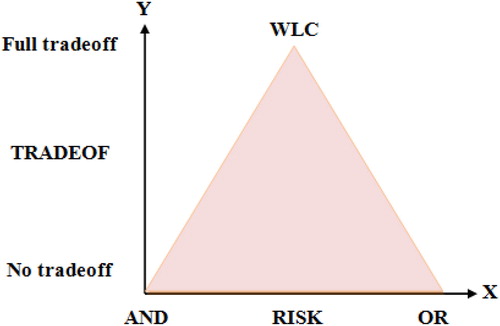
In Figure 5, the x-axis is the maximum precaution, and the y-axis represents the trade-off between criteria. Weighted linear combination (WLC) is based on the weighted average, in which the criteria are combined in a standard common numerical interval using the weighted average . The ordered weighted average method can provide prediction maps and shapes for various evaluations by varying the order and benchmark parameters (Ferretti and Pomarico 2013).

OWA is defined as a hybrid technique with an $\mathit{ith}$ location, a set of order weights $v=v_1,\mathrm{ }{v}_2,\dots ,v_n\mathrm{ }(v_j^{°}[0,\mathrm{ }1],\mathrm{ }j=1,\mathrm{ }2,\dots ,n,\mathrm{ }\mathrm{and}\mathrm{ }{\sum }_{j=1}^{n}wj=1$) and a set of criteria weights $w=w1,\mathrm{ }w2,\mathrm{ }{w}_n\mathrm{ }({wj}^{°}[0,\mathrm{ }1],\mathrm{ }\mathrm{and}\mathrm{ }{\sum }_{j=1}^{n}wj=1)\mathrm{ }$(Motlagh and Sayadi 2015).

In general, the OWA model with two parameters, AND ORness and TRADEOFF, is defined as follows: (15) $$\mathrm{ANDness}=\left(\frac{1}{n-1\mathrm{ }}\right)\sum \mathrm{ }\left(\right(\mathrm{ }n-\mathrm{i}\mathrm{ }){\mathrm{W}}_{\mathrm{orderi}}\mathrm{ }$$(15) (16) $$\mathrm{ORness}=1-\mathrm{ANDness}\mathrm{ }$$(16) (17) $$\mathrm{TRADEOFF}=1-\mathrm{ }\sqrt{\frac{n\mathrm{ }(\sum {\mathrm{W}}_{\text{order i}}-{1/n)}^2}{n-1}}\mathrm{ }$$(17) where $n$ is the number of factors, $i$ is their order and the ${\mathrm{W}}_{\mathrm{orderi}}$ is the weight of the order factor.

The OWA operator is calculated with the following equation: (18) $${\mathit{OWA}}_{\mathrm{i}}=\sum \left(\frac{\mathit{\text{Wj Vj}}}{\sum _{j=1}^n\mathit{\text{Wj Vj}}}\right) \mathit{Zij}\mathrm{ }$$(18) where $\mathit{Zin} \ge \dots \ge Zi1$ is specified by the order of the criterion ($\mathit{xij}$),$Vj\mathrm{ }$ is the weight of the order, and $Wj$ is the weight criterion (Malczewski 2006).

The OWA model requires standardized layers. We used a standardization method based on the minimum and maximum factor values (Equations (18)(18) $${\mathit{OWA}}_{\mathrm{i}}=\sum \left(\frac{\mathit{\text{Wj Vj}}}{\sum _{j=1}^n\mathit{\text{Wj Vj}}}\right) \mathit{Zij}\mathrm{ }$$(18) and (19)(19) $$a_{ij }= \frac{S_{ij}- S_j^{\mathit{min}}}{S_j^{\mathit{max}}- S_j^{\mathit{min}}}\mathrm{ }$$(19) ). Therefore, the following two equations are used to convert crude values to standard values: (19) $$a_{ij }= \frac{S_{ij}- S_j^{\mathit{min}}}{S_j^{\mathit{max}}- S_j^{\mathit{min}}}\mathrm{ }$$(19) (20) $$a_{ij }= \frac{S_j^{\mathit{max}}- S_{ij}}{S_j^{\mathit{max}}- S_j^{\mathit{min}}}\mathrm{ }$$(20) where $S_{ij}\mathrm{ }$ is the value of $i$ for the criterion $j,$${ S}_j^{\mathit{min}}$ is the lowest value for the criterion $j$ and $S_j^{\mathit{max}}$ is the highest raw value for the criterion $j$ .

In this study, the weights of factors obtained using the ANP method (Figure 6) and (Table 4) were calculated using Equation (21)(21) $$V_j=\mathrm{ }{\left(\sum _{j=1}^{n}wj\right)}^{\alpha }-\mathrm{ }{\left(\sum _{j=1}^{n-1}wj\right)}^{\alpha }\mathrm{ }$$(21) . Then, the order weights obtained from OWA were multiplied by the ordered quantities (Table 5). (21) $$V_j=\mathrm{ }{\left(\sum _{j=1}^{n}wj\right)}^{\alpha }-\mathrm{ }{\left(\sum _{j=1}^{n-1}wj\right)}^{\alpha }\mathrm{ }$$(21) where $wj$ is the criterion weight, and $\alpha$ is the degree of optimism OWA obtained from Table 5.

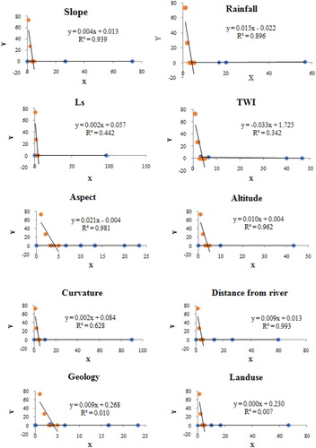
Figure 6. Linear regression between the percentage of flood points and the frequency ratio (X = FR index and Y = Percentage of points in each class) (Blue points: flood percentage in each class and yellow points: FR percentage in each class).

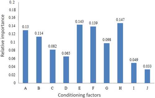
Table 4. EBF results for flood factors.

Factor	Value	N (${\mathit{C}}_{\mathit{ji}}$)	N (${\mathit{C}}_{\mathit{ji}}\cap \mathit{D}$)	∑${\mathit{C}}_{\mathit{ji}}$ B	Bel
Slope	>15	5634655	22	1.76	0.7308
	15–30	3305997	8	0.65	0.2710
	30–45	295673	0	0.00	0.0000
	45–60	5929	0	0.00	0.0000
	>60	1163	0	0.00	0.0000
Rainfall	<330	643850	1	0.46	0.0514
	330–370	775290	1	0.38	0.0420
	370–410	2092066	5	0.68	0.0763
	410–450	4302804	6	0.29	0.0320
	>450	1429407	17	7.15	0.7978
Slope length	<11	8917176	29	1.06	0.5279
	11–22	324629	1	0.95	0.4713
	22–33	1450	0	0.00	0.0000
	33–44	126	0	0.00	0.0000
	>44	36	0	0.00	0.0000
TWI	<6	5004183	12	0.56	0.0266
	6–10	3656518	14	1.34	0.0629
	10–14	457952	1	0.66	0.0311
	14–16	98360	2	6.64	0.3127
	>16	26404	1	12.04	0.5667
Slope aspect	Flat	8226	0	0.00	0.0000
	North	1367816	4	0.89	0.1055
	Northeast	1145484	2	0.50	0.0601
	East	1068949	3	0.85	0.1012
	Southeast	1134575	4	1.10	0.1309
	South	1227278	3	0.73	0.0864
	Southwest	1051979	6	1.95	0.2317
	West	1080619	1	0.26	0.0310
	Northwest	1158491	7	2.12	0.2529
Altitude	<1600	2022537	13	2.73	0.5343
	1600–1800	2662218	13	1.89	0.3699
	1800–2000	2330958	3	0.33	0.0645
	2000–2200	1642852	1	0.16	0.0312
	>2200	584852	0	0.00	0.0000
Plan curvature	Concave	646779	0	0.00	0.0000
	Flat	7427818	27	2.20	0.7407
	Convex	1168820	3	0.77	0.2584
Distance from river	<600	2561908	18	3.91	0.6998
	600–1200	2284278	8	1.11	0.1982
	1200–1800	1974536	4	0.57	0.1013
	1800–2400	1591706	0	0.00	0.0000
	>2400	830989	0	0.00	0.0000
Geology	CI	33025	0	0.00	0.0000
	E21	42601	0	0.00	0.0000
	EK	51793	0	0.00	0.0000
	Kpef	1385458	5	1.13	0.0411
	Kabv	55005	0	0.00	0.0000
	Kfsh	1091642	5	1.49	0.0542
	KISM	18921	0	0.00	0.0000
	Ku	1323043	5	1.20	0.0434
	oMqI	3357	0	0.00	0.0000
	oqtdg	252771	1	1.23	0.0445
	Pagr	193046	1	1.62	0.0586
	Pd	552771	1	0.54	0.0197
	PeEf	267030	1	1.16	0.0420
	PeI	160606	0	0.00	0.0000
	Pims	2987709	7	0.64	0.0231
	Pr	32478	0	0.00	0.0000
	qft2	1648	0	0.00	0.0000
	TRIs	289281	0	0.00	0.0000
	TRJvm	133928	0	0.00	0.0000
	pCgr	230135	2	2.80	0.1014
	pCmb	112673	1	2.79	0.1013
	pCmt1	24496	1	12.98	0.4705
Land use/Land cover	Garden	5658174	20	1.27	0.1850
	Good rangelands	106055	1	2.97	0.4337
	Dry farming	1366819	3	0.64	0.0935
	Moderate rangelands	1737745	5	0.86	0.1261
	Poor rangelands	280480	1	1.10	0.1609
	Urban area	31637	0	0.00	0.0000
	Water range	62507	0	0.00	0.0000

Table 5. The order weights and the corresponding decision.

$\mathit{\alpha }$	Quantifier	Order weights	GIS combination procedure	ORness	Trade-Off
$\alpha \to 0$	At least one	$V_{i1}=1, V_{ik}=0, (1<k\le n)$	OWA (OR)	1	0
$\alpha =0.1$	$\text{At least a few}$	a	OWA	A	a
$\alpha =0.5$	$\text{A few}$	a	OWA	A	a
$\alpha =1$	$\mathrm{Half}$	$V_{ik}=1, V_{i1}=0, (1\le k\le n)$	OWA (WLC)	0.5	1
$\alpha =2$	$\mathrm{Most}$	a	OWA	A	a
$\alpha =10$	$\text{Almost all}$	a	OWA	A	a
$\alpha \mathrm{ }\to \mathrm{ }\mathrm{\infty }$	$\mathrm{All}$	$V_{in}=1, V_{ik}=0, (1\le k<n)$	OWA (AND)	0	0

The OWA technique is an embedded type of multi-criteria decision-making and enables geographic information systems to perform data analysis and decision-making. Input for this model is raster maps of the study area and descriptive tables.

2.4. Models validation

The Receiver Operating Characteristic (ROC) curve was used to evaluate the produced models. The ROC curve is a graphical representation of the balance between the negative and positive error rates for each possible value and is based on the set of pair points (X and Y) calculated using Equations (22)(22) $$X=1-\mathrm{ }\left[\frac{TN}{TN-FP}\right]\mathrm{ }$$(22) and (23)(23) $$Y=\mathrm{ }\left[\frac{TP}{TP-FN}\right]\mathrm{ }$$(23) . The X and Y were obtained from the comparison matrix and varied between 0 and 1 (Yariyan et al. 2020a). The area under the ROC curve is called the area under the curve (AUC). The AUC gives the value of the system’s prediction by describing its ability to accurately predict events (floods) and non-events (non-floods). The values are a percentage of true reality and the percentage of false reality of the graph is calculated according to the following equations. (22) $$X=1-\mathrm{ }\left[\frac{TN}{TN-FP}\right]\mathrm{ }$$(22) (23) $$Y=\mathrm{ }\left[\frac{TP}{TP-FN}\right]\mathrm{ }$$(23) where $TN, FP, TP,$ and $FN$ are true negative, false positive, true positive, and false negative (Leman et al. 2020).

2.5. Multi-collinearity test of geo-environmental factors

Multi-linearity (or collinearity) is a type of statistical phenomenon in multiple linear regression analyses in which two (or more) predictor variables are related or interrelated (Kroll and Song 2013). It is necessary to choose a method that can predict the impact of variables independently in such research (Gudiyangada Nachappa et al. 2019; Yousefi et al. 2020). In this study, the linearity of flood conditioning factors was investigated using the Variance Inflation Factor (VIF) and Tolerance (TOL). If the TOL <0.1 or the VIF ≥ 5, there is a linear relationship between the conditioning factors (Equations (24)(24) $$\mathrm{TOL}=1-\mathrm{ }{\mathrm{R}}_{\mathrm{j}}^2$$(24) and (25)(25) $$\mathrm{VIF}=\mathrm{ }\frac{1}{\mathrm{TOL}}\mathrm{ }$$(25) ) (24) $$\mathrm{TOL}=1-\mathrm{ }{\mathrm{R}}_{\mathrm{j}}^2$$(24) (25) $$\mathrm{VIF}=\mathrm{ }\frac{1}{\mathrm{TOL}}\mathrm{ }$$(25) where ${\mathrm{R}}_{\mathrm{j}}^2$ is the coefficient of determination of the regression model .

3. Results

3.1. Multi-collinearity test of geo-environmental factors

The results of the multi-collinearity analysis showed it is not multi-collinearity between the conditioning factors and the effective factors in the flood risk mapping (Table 6). The highest VIF and the lowest TOL were 1.762 and 0.567, respectively.

Table 6. Multi-collinearity of flood conditioning factors.

Parameter	Collinearity statistics
	TOL	VIF
Slope	0.567	1.762
Rainfall	0.583	1.713
Slope length	0.755	1.324
TWI	0.592	1.688
Aspect	0.869	1.150
Altitude	0.662	1.510
Curvature	0.668	1.496
Distance from river	0.792	1.262
Geology	0.800	1.249
LU/LC	0.697	1.434

3.2. Result of the analytic network process (ANP) model

The results of the ANP indicated that the distance from river (H) has the highest weight of all the factors (Figure 7). Following the distance from river (0.147), the order of weights of the other factors is as follows: aspect (0.143), altitude (0.139), slope (0.13), rainfall (0.114), curvature (0.098), LS (0.082), TWI (0.065), geology (0.049), and LU/LC (0.033) (Figure 6). The value of the compatibility index (CR) is 0.00041 (less than 0.1), which indicates that there is no incompatibility between the factors and the results are thus valid.

Figure 7. The relative importance of conditioning factors in the ANP model. A: Slope, B: Rainfall, C: Slope Length, D: TWI, E: Aspect, F: Altitude, G: Curvature, H: Distance from river, I: Geology, J: Land use.

Based on the results of the ANP and the importance of different conditioning factors, we could suggest the following general equation for a flood susceptibility map: (26) $$\mathit{FSM}=0.13A+0.114B+0.082C+0.065D+0.143E+0.139F+0.098G+0.147H+0.049I+0.033J\mathrm{ }$$(26) where A, B, C, D, E, F, G, H, I and G are slope, rainfall, slope length, TWI, aspect, altitude, curvature, distance from river, geology, and LU/LC, respectively. The values of A-G are obtained based on the FR, EBF, and OWA. This new approach aims to determine the weights of factors with high accuracy because the initial weight of the factors is determined objectively.

3.3. Frequency ratios for different classes of flood condition factors

The factors with the highest value of frequency ratio are shown in Table 6 in bold.

Among of different classes of the slope, rainfall, slope length, TWI, aspect, altitude, curvature, distance from river, geology and LU/LC, >15%, >450 mm, <11, 14–24, northwest, <1600 m, flat, <600 m, pCmt1, good range shows maximum frequency ratio, respectively (Table 6).

In Figure 6, the x-axis represents the percentage of flood occurrence points in each class and the y-axis represents the calculated FR values in each class. By calculating the coefficient of determination for each of the regression relationships, the initial weight of each factor was determined according to the R coefficient on a scale of 1 to 9. So, the higher the${\text{ R}}^2,$ the higher the weighting factor. Then, Super decisions software was used to implement the ANP model and to form a pairwise comparisons matrix.

3.4. Weight of different classes of flood condition factors based on EBF

In Table 3, $N (C_{ji})$ is the number of pixel units in each class, $N (C_{ji} \cap D)$ is the number of flood points in each class, and $Wi$ represents the weight of the ANP. After applying the Bel weights to each class of flood factors, the ANP-EBF hybrid model was implemented based on Equation (24)(24) $$\mathrm{TOL}=1-\mathrm{ }{\mathrm{R}}_{\mathrm{j}}^2$$(24) .

Then, to implement the EBF method to integrate different factors to reduce uncertainty in flood risk mapping, the values (Bel) were calculated for each class of effective flood factors (Table 4). For the combined modelling, all flood conditioning factors were classified based on the EBF weight obtained from Bel.

3.5. Flood susceptibility modelling (FSM)

By using the relationship between the flood points and the conditioning factors associated with floods, we created flood susceptibility maps using the hybrid method of the ANP (Figure 8 and Equation (26)(26) $$\mathit{FSM}=0.13A+0.114B+0.082C+0.065D+0.143E+0.139F+0.098G+0.147H+0.049I+0.033J\mathrm{ }$$(26) ) with FR (Table 3) and EBF (Table 4) models. Therefore, the weights of FR and EBF of each susceptibility class of each factor (Tables 3 and 4) were applied in Equation (25)(25) $$\mathrm{VIF}=\mathrm{ }\frac{1}{\mathrm{TOL}}\mathrm{ }$$(25) . The result of executing the above command in ArcGIS software is the flood risk map in the interval 0–1 (Figure 8(a,b)).

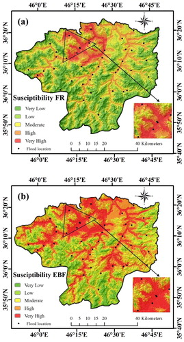
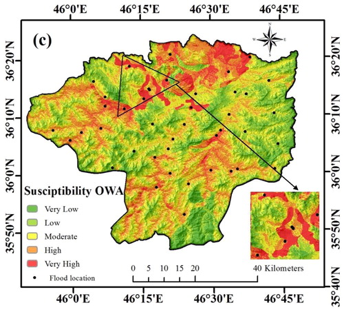
Figure 8. Flood susceptibility map. (a) ANP-FR hybrid model, (b) ANP-EBF hybrid model, and (c) ANP-OWA hybrid model.

We implemented the OWA model using ANP weights, the weights of the factors, and the order weights. This second set of weights allows for direct control over the risk level. The order weight is a set of weights assigned to a given location (pixels). Applying the weight of the order based on the grading factors affects the minimum to the maximum value for each location. After standardizing and entering layers into the IDRISI software, we implemented the OWA analytical model and the result was a flood risk map with values between 0 and 1 (Figure 8(c)).

3.6. Validation

In the ROC curve from the area under the curve (AUC), standard error (SE), and confidence interval (CI) were used to evaluate the efficiency of the models (Figure 9). Evaluation of the models showed that the hybrid models ANP-FR, ANP-EBF, and ANP-OWA yielded performance coefficients of 91%, 95.1%, and 89.6%, respectively. These values indicate the good performance of the hybrid models for flood risk assessment in the study area. However, the ANP-EBF model with the highest accuracy (AUC = 0.951, SE = 0.0494) compared to the ANP-FR (AUC = 0.91, SE = 0.0833), and ANP-OWA (AUC = 0.896, SE = 0.0632) models is best suited to determine the risk of flooding in the region (Table 7). Evaluation statistics of the applied methods are shown in Table 4. According to the results shown in Table 4, the ANP-FR has the lowest standard error (0.49) compared to the ANP-EBF (0.083) and ANP-WOA (0.063) models.

Figure 9. The area under curve (AUC) values for hybrid models (ANP-FR), (ANP-EBF), and (ANP-OWA).

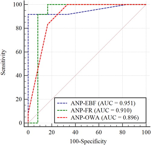
Table 7. ROC curve validation results.

Variable	AUC	SE	95% CI
ANP-EBF	0.951	0.0494	0.779 to 0.998
ANP-FR	0.910	0.0833	0.721 to 0.987
ANP-OWA	0.896	0.0632	0.703 to 0.982

4. Discussion

Evaluation of the performance of the hybrid statistical models and multi-criteria decision-making showed that the ANP-EBF, ANP-FR, and ANP-OWA models perform well in flood hazard zoning in the Saqqez watershed. We evaluated the performance of the hybrid models based on the AUC, SE and CI criteria, which showed that the ANP-EBF hybrid model was able to map the flood susceptibility with an AUC = 95.1%, SE = 0.0494 and CI = 0.779 to 0.998 efficiency coefficient, compared to the slightly lower values of 91.0% and 89.6% achieved by the ANP-FR and ANP-OWA models, respectively. Because the ANP model is a comprehensive technique that allows all direct and indirect factors to influence decision-making, its combination with other models increases their accuracy. ANP method allows for more complex relationships between decision levels and features to be evaluated because levels do not require a strict hierarchical structure. Because of the interdependence characteristics that exist in natural hazards such as floods, it is also important to consider the interrelationships between the criteria in the decision-making (Alilou et al. 2019; Kanani-Sadat et al. 2019). The ANP method allows us to examine the interdependencies between the criteria levels and is, therefore, an appropriate tool for multi-criteria decision-making (Sun et al. 2016). Our results are in line with the results of Wang et al. (2018); Alilou et al. (2019); Dano et al. (2019) who also found in their studies that combining multi-criteria decision-making methods with statistical methods is effective in better modelling and increasing the efficiency of individual methods. Although, the combination of the ANP model with FR and OWA algorithms contains good accuracy, the findings of our study indicate that the accuracy of the ANP-EBF hybrid model is suitable for identifying flood-prone areas of the Saqqez watershed. This can show the high accuracy of Bel values from the EBF model compared to FR values for each class of factors. For example, Tehrany et al. (2019) used the combination of the EBF algorithm with the SVM model to flood susceptibility mapping, and the results of their study indicate the high accuracy of the SVM-EBF combination. Also, based on the results of the study (Arabameri et al. 2019), the EBF algorithm has a better performance than FR in predicting flood sensitivity. In addition to the above, according to research (Chowdhuri et al. 2020), the EBF-LR combination for predicting flood sensitivity also has the highest accuracy. These can confirm the findings of our study. Therefore, the use of an EBF in flood risk assessment is useful and reliable.

Since most of the floods are caused by the flooding of the main river channel, the distance from the river is one of the most important factors in the flood sensitivity analysis. Areas close to the river are more vulnerable to flooding due to the proximity to the mainstream and rapid response to floods (Chapi et al. 2017; Moradi et al. 2019). Our results showed that the 0–600 meters class in the factor of distance from river has the highest flood risk. Shafizadeh-Moghadam et al. (2018) showed in their study, that the distance from the river factor is one of the most important variables to determine the risk of flooding and that the areas close to the river are most sensitive to flooding. In the aspect factor with its high importance in flood occurrence (0.143), the northwest class has the highest sensitivity (FR = 1.86, Bel = 0.2529) for the flood. By comparing the maps obtained from the models and Figure 4(e), the accuracy of these results can be realized. The flood sensitivity map of the study area shows the northern part of Saqqez City is more sensitive to flooding. Observing Figure 4(f), we find that the northern parts of the study area with the lowest altitude are more prone to floods. This is completely consistent with the analytical calculations of the FR algorithm for the altitude factor. So that the highest sensitivity in the altitude class is less than 1600 meters. One of the primary reasons for this is the possibility of more concentrated water flow at low altitudes. Our result is consistent with the results of Fernández and Lutz (2010); Tehrany et al. (2015); Termeh et al. (2018); Costache et al. (2020) who also stated in their study that with increasing altitude, the sensitivity of the classes to flooding decreases. Examination of the slope factor shows that the highest effective weight factor in flood sensitivity the class <15%. The higher concentration of water at low slopes increases the sensitivity and the risk of flooding. Vojtek and Vojteková (2019) found that one of the effective factors in flood sensitivity is the slope angle and that low slopes are very prone to flooding. As our calculations show, high FR and Bel values are in low slope classes. Therefore, it can be found that by establishing a linear relationship to reach the final weight through the FR algorithm and slope factor sensitivity classes, the high importance of the slope factor (0.13) has been calculated correctly. Therefore, the findings of the study (Khosravi et al. 2018) also emphasize the high importance of the factors of distance from the river, slope, and altitude in the occurrence of floods, which can confirm the weights calculated for these factors in our study.

Rainfall is one of the most important influencing factors in flood sensitivity. According to the rainfall map of Saqqez City, areas with precipitation of more than 450 mm in the northern part of Saqqez City are more prone to flooding. Also, according to the results of the ANP model, the rainfall factor with a weight of 0.114 is very important in the occurrence of floods. In addition, the obtained FR and Bel values for rainfall sensitivity classes indicate the presence of high sensitivity in the class> 450 mm. Therefore, the correspondence of the results in Tables 3 and 4, Figure 7, and the output maps (Figure 8), indicates the high importance of the rainfall factor and the complete agreement of the calculations. After Slope, Altitude, Distance from river, Rainfall, and Aspect factors, the curvature factor is the most important in flood occurrence. Relationships between flood locations and sensitivity classes indicate high sensitivity in the Flat class. Therefore, the prediction of floods on slopes and low altitudes and flat places in this study indicates the high accuracy of calculations and results. The relationship between FR and Bel values in the slope length factor sensitivity classes indicates high sensitivity in class <11. These calculations are fully correlated with the values obtained for the slope factor and the sensitivity at low slopes. So that on a slope with a lower degree and length, the degree of flood sensitivity is higher.

Investigation of the effect of TWI on flood sensitivity showed that areas with high TWI had more of an effect on flood sensitivity in the study area. As the TWI shows the distribution of moisture distribution in different parts, increasing this index increases soil moisture content and increases the probability of flooding. TWI is one of the most important factors affecting flood and that areas with a high TWI are highly sensitive to flooding. The results of Tables 3 and 4 for the TWI factor also show in the classes with the highest value (>16), high sensitivity. The relationship between flood and geological factors in this study shows the high sensitivity of Moderate—grade, regional metamorphic rocks (pCmt1) to flood. In general, the PC group was more effective. So that, after pCmt1, pCmb (Marble) and pCgr (Precambrian granite to granodiorite) groups had the highest flood sensitivity, respectively.

Investigation of the effect of land use/land cover on flood sensitivity in Saqqez City showed that orchards and agricultural lands have a more significant effect on flooding than other land-use types. As agricultural and orchard land-use types are extensive near the main river and downstream of the basin, these areas are most affected by flooding and inundation. So that floods near agricultural lands, despite having nutrients, can be one of the factors of quality and growth of agricultural products.

5. Conclusion

In this study, flood risk zoning was determined using a combination of statistical methods (FR, EBF, and OWA) and a multi-criteria decision-making model (ANP) in the Saqqez watershed in Kurdistan Province, which is one of the most flood-prone areas in this province. The environmental variables we used to model flood susceptibility were altitude, slope, aspect, distance from river, rainfall, TWI, LS, plan curvature, LU/LC, and lithology. The results of the combination of the statistical method of FR and ANP (ANP-FR) showed that this hybrid method was more efficient than the ANP-EBF and ANP-OWA methods. The analysis of the importance of factors using ANP showed that the variables of distance to river, aspect, and altitude were the more important in determining the flood zone in this area. The results of flood hazard zoning showed that the northern areas of the watershed are highly susceptible to floods, and these are generally are low-lying areas close to the river. Today, financial bottlenecks in watershed management require that a watershed be properly budgeted, and that flood protection and management measures are prioritized to maximize effectiveness. Therefore, surveying, analyzing, and mapping flood susceptibility zones can play an important role in better management of watersheds, budget allocation, and organization of structural and non-structural operations. Moreover, given the fact that, during the last decades, climate change creates the premises for severe flood events across many regions of the globe, we consider that flood susceptibility estimation through highly accurate models is mandatory. Therefore, since the accuracy of the three hybrid models, used in the present study, exceed 89% we have a higher degree of confidence that the present methodology can be successfully used also in other areas, across the Earth, which is exposed to flood occurrence. Thus, the novel hybrid models and the high accuracies of the methods make from this manuscript valuable research which will be of great interest for the potential readers across the entire globe.

Author contributions

Conceptualization, P.Y., M.A. A.T.H, and O.G; methodology, P.Y., and R.A.A; software, P.Y; validation, P.Y., M.A., and R.C; data curation, P.Y., M.A., and S.J; formal analysis, P.Y; writing—original draft preparation, P.Y., M.A., and O.G; writing—review and editing, R.A.A, R.C, O.G, and T.B; supervision, T.B; funding acquisition, T.B.

Acknowledgments

We would like to thank four anonymous reviewers for their valuable comments. Open Access Funding by the Austrian Science Fund (FWF).

Disclosure statement

The authors declare no conflict of interest.

Data availability statement

The data that support the findings of this study are available from the corresponding author, O.G, upon reasonable request.

Additional information

Funding

This research was partly funded by the Open Access Funding of Austrian Science Fund (FWF) through the GISscience Doctoral College (DK W 1237-N23).

References

- Ahmadlou M, Karimi M, Alizadeh S, Shirzadi A, Parvinnejhad D, Shahabi H, Panahi M. 2019. Flood susceptibility assessment using integration of adaptive network-based fuzzy inference system (ANFIS) and biogeography-based optimization (BBO) and BAT algorithms (BA). Geocarto Int. 34(11):1252–1272.
- Ali SA, Parvin F, Pham QB, Vojtek M, Vojteková J, Costache R, Linh NTT, Nguyen HQ, Ahmad A, Ghorbani MA. 2020. GIS-based comparative assessment of flood susceptibility mapping using hybrid multi-criteria decision-making approach, naïve Bayes tree, bivariate statistics and logistic regression: a case of Topľa basin, Slovakia. Ecol Indic. 117:106620.
- Alilou H, Rahmati O, Singh VP, Choubin B, Pradhan B, Keesstra S, Ghiasi SS, Sadeghi SH. 2019. Evaluation of watershed health using Fuzzy-ANP approach considering geo-environmental and topo-hydrological criteria. J Environ Manage. 232:22–36.
- Alizadeh M, Ngah I, Hashim M, Pradhan B, Pour AB. 2018. A hybrid analytic network process and artificial neural network (ANP-ANN) model for urban earthquake vulnerability assessment. Remote Sensing. 10(6):975.
- Al-Juaidi AE, Nassar AM, Al-Juaidi OE. 2018. Evaluation of flood susceptibility mapping using logistic regression and GIS conditioning factors. Arab J Geosci. 11(24):765.
- Arabameri A, Rezaei K, Cerdà A, Conoscenti C, Kalantari Z. 2019. A comparison of statistical methods and multi-criteria decision making to map flood hazard susceptibility in Northern Iran. Sci Total Environ. 660:443–458.
- Avand M, Janizadeh S, Naghibi SA, Pourghasemi HR, Khosrobeigi Bozchaloei S, Blaschke T. 2019. A comparative assessment of Random Forest and k-Nearest Neighbor classifiers for gully erosion susceptibility mapping. Water. 11:2076.
- Avand M, Janizadeh S, Tien Bui D, Pham VH, Ngo PTT, Nhu V-H. 2020. A tree-based intelligence ensemble approach for spatial prediction of potential groundwater. Int J Digital Earth. 10. 1–22.
- Bathrellos GD, Skilodimou HD, Soukis K, Koskeridou E. 2018. Temporal and spatial analysis of flood occurrences in the drainage basin of Pinios river (Thessaly, Central Greece). Land. 7(3):106.
- Bui DT, Ngo P-TT, Pham TD, Jaafari A, Minh NQ, Hoa PV, Samui P. 2019a. A novel hybrid approach based on a swarm intelligence optimized extreme learning machine for flash flood susceptibility mapping. Catena. 179:184–196.
- Bui DT, Pradhan B, Lofman O, Revhaug I, Dick OB. 2012. Spatial prediction of landslide hazards in Hoa Binh province (Vietnam): a comparative assessment of the efficacy of evidential belief functions and fuzzy logic models. Catena. 96:28–40.
- Bui DT, Tsangaratos P, Ngo P-TT, Pham TD, Pham BT. 2019b. Flash flood susceptibility modeling using an optimized fuzzy rule based feature selection technique and tree based ensemble methods. Sci Total Environ. 668:1038–1054.
- Chapi K, Singh VP, Shirzadi A, Shahabi H, Bui DT, Pham BT, Khosravi K. 2017. A novel hybrid artificial intelligence approach for flood susceptibility assessment. Environ Modell Software. 95:229–245.
- Chen C-Y, Yu F-C. 2011. Morphometric analysis of debris flows and their source areas using GIS. Geomorphology. 129(3-4):387–397.
- Chen W, Hong H, Li S, Shahabi H, Wang Y, Wang X, Ahmad BB. 2019. Flood susceptibility modelling using novel hybrid approach of reduced-error pruning trees with bagging and random subspace ensembles. J Hydrol. 575:864–873.
- Choubin B, Moradi E, Golshan M, Adamowski J, Sajedi-Hosseini F, Mosavi A. 2019. An ensemble prediction of flood susceptibility using multivariate discriminant analysis, classification and regression trees, and support vector machines. Sci Total Environ. 651(Pt 2):2087–2096.
- Chowdhuri I, Pal SC, Chakrabortty R. 2020. Flood susceptibility mapping by ensemble evidential belief function and binomial logistic regression model on river basin of eastern India. Adv Space Res. 65(5):1466–1489.
- Costache R, Pham QB, Avand M, Linh NTT, Vojtek M, Vojteková J, Lee S, Khoi DN, Nhi PTT, Dung TD. 2020. Novel hybrid models between bivariate statistics, artificial neural networks and boosting algorithms for flood susceptibility assessment. J Environ Manage. 265:110485.
- Costache R. 2019a. Flash-flood potential index mapping using weights of evidence, decision trees models and their novel hybrid integration. Stoch Environ Res Risk Assess. 33(7):1375–1402.
- Costache R. 2019b. Flood susceptibility assessment by using bivariate statistics and machine learning models-a useful tool for flood risk management. Water Resour Manage. 33(9):3239–3256.
- Dammalage T, Jayasinghe N. 2019. Land-use change and its impact on urban flooding: a case study on Colombo District Flood on May 2016. Eng Technol Appl Sci Res. 9:3887–3891.
- Dano UL, Balogun A-L, Matori A-N, Wan Yusouf K, Abubakar IR, Mohamed S, Ahmed M, Aina YA, Pradhan B. 2019. Flood susceptibility mapping using GIS-based analytic network process: A case study of Perlis, Malaysia. Water. 11(3):615.
- Darabi H, Choubin B, Rahmati O, Haghighi AT, Pradhan B, Kløve B. 2019. Urban flood risk mapping using the GARP and QUEST models: a comparative study of machine learning techniques. J Hydrol. 569:142–154.
- Das B, Pal SC, Malik S, Chakrabortty R. 2019. Living with floods through geospatial approach: a case study of Arambag CD Block of Hugli District, West Bengal, India. SN Appl Sci. 1(4):329.
- Das B, Pal SC, Malik S. 2018. Assessment of flood hazard in a riverine tract between Damodar and Dwarkeswar River, Hugli District, West Bengal, India. Spat Inf Res. 26(1):91–101.
- Das S. 2018. Geographic information system and AHP-based flood hazard zonation of Vaitarna basin, Maharashtra, India. Arab J Geosci. 11(19):576.
- Doocy S, Daniels A, Packer C, Dick A, Kirsch TD. 2013. The human impact of earthquakes: a historical review of events 1980-2009 and systematic literature review. PLoS Currents. 5: 1–9.
- Fernández D, Lutz M. 2010. Urban flood hazard zoning in Tucumán Province, Argentina, using GIS and multicriteria decision analysis. Eng Geol. 111(1-4):90–98.
- Ferretti V, Pomarico S. 2013. Ecological land suitability analysis through spatial indicators: an application of the Analytic Network Process technique and Ordered Weighted Average approach. Ecol Indic. 34:507–519.
- Ghorbani Nejad S, Falah F, Daneshfar M, Haghizadeh A, Rahmati O. 2016. Delineation of groundwater potential zones using remote sensing and GIS-based data-driven models. Geocarto Int. 32:1–187.
- Ghorbanzadeh O, Blaschke T, Gholamnia K, Aryal J. 2019a. Forest fire susceptibility and risk mapping using social/infrastructural vulnerability and environmental variables. Fire. 2(3):50.
- Ghorbanzadeh O, Feizizadeh B, Blaschke T. 2018a. An interval matrix method used to optimize the decision matrix in AHP technique for land subsidence susceptibility mapping. Environ Earth Sci. 77(16):584.
- Ghorbanzadeh O, Feizizadeh B, Blaschke T. 2018b. Multi-criteria risk evaluation by integrating an analytical network process approach into GIS-based sensitivity and uncertainty analyses. Geomatics Nat Hazards Risk. 9(1):127–151.
- Ghorbanzadeh O, Moslem S, Blaschke T, Duleba S. 2019b. Sustainable urban transport planning considering different stakeholder groups by an interval-AHP decision support model. Sustainability. 11(1):9.
- Ghorbanzadeh O, Valizadeh Kamran K, Blaschke T, Aryal J, Naboureh A, Einali J, Bian J. 2019c. Spatial prediction of wildfire susceptibility using field survey GPS data and machine learning approaches. Fire. 2(3):43.
- Gudiyangada Nachappa T, Tavakkoli Piralilou S, Ghorbanzadeh O, Shahabi H, Blaschke T. 2019. Landslide susceptibility mapping for Austria using Geons and optimization with the Dempster-Shafer theory. Appl Sci. 9(24):5393.
- Ha MH, Yang Z, Heo MW. 2017. A new hybrid decision making framework for prioritising port performance improvement strategies. Asian J Shipping Logistics. 33(3):105–116.
- Hölting B, Coldewey WG. 2019. Surface water infiltration. In: Hydrogeology. Springer; Berlin, Heidelberg, p. 33–37.
- Hong H, Tsangaratos P, Ilia I, Liu J, Zhu A-X, Chen W. 2018. Application of fuzzy weight of evidence and data mining techniques in construction of flood susceptibility map of Poyang County, China. Sci Total Environ. 625:575–588.
- Janizadeh S, Avand M, Jaafari A, Phong TV, Bayat M, Ahmadisharaf E, Prakash I, Pham BT, Lee S. 2019. Prediction success of machine learning methods for flash flood susceptibility mapping in the Tafresh Watershed, Iran. Sustainability. 11(19):5426.
- Kanani-Sadat Y, Arabsheibani R, Karimipour F, Nasseri M. 2019. A new approach to flood susceptibility assessment in data-scarce and ungauged regions based on GIS-based hybrid multi criteria decision-making method. J Hydrol. 572:17–31.
- Kazakis N, Kougias I, Patsialis T. 2015. Assessment of flood hazard areas at a regional scale using an index-based approach and analytical hierarchy process: application in Rhodope-Evros region, Greece. Sci Total Environ. 538:555–563.
- Khosravi K, Pham BT, Chapi K, Shirzadi A, Shahabi H, Revhaug I, Prakash I, Bui DT. 2018. A comparative assessment of decision trees algorithms for flash flood susceptibility modeling at Haraz watershed, northern Iran. Sci Total Environ. 627:744–755.
- Khosravi K, Shahabi H, Pham BT, Adamowski J, Shirzadi A, Pradhan B, Dou J, Ly H-B, Gróf G, Ho HL, et al. 2019. A comparative assessment of flood susceptibility modeling using multi-criteria decision-making analysis and machine learning methods. J Hydrol. 573:311–323.
- Kroll CN, Song P. 2013. Impact of multicollinearity on small sample hydrologic regression models. Water Resour Res. 49(6):3756–3769.
- Kundzewicz ZW, Kanae S, Seneviratne SI, Handmer J, Nicholls N, Peduzzi P, Mechler R, Bouwer LM, Arnell N, Mach K, et al. 2014. Flood risk and climate change: global and regional perspectives. Hydrol Sci J. 59(1):1–28.
- Lee S, Lee S, Lee M-J, Jung H-S. 2018. Spatial assessment of urban flood susceptibility using data mining and geographic information System (GIS) tools. Sustainability. 10(3):648.
- Leman R, Tubeuf H, Raad S, Tournier I, Derambure C, Lanos R, Gaildrat P, Castelain G, Hauchard J, Killian A, et al. 2020. Assessment of branch point prediction tools to predict physiological branch points and their alteration by variants. BMC Genomics. 21(1):86.
- Liu J-f, Li J, Liu J, Cao R-y. 2008. Integrated GIS/AHP-based flood risk assessment: a case study of Huaihe River Basin in China. J Nat Disasters. 17:110–114.
- Malczewski J. 2006. Ordered weighted averaging with fuzzy quantifiers: GIS-based multicriteria evaluation for land-use suitability analysis. IJAEO. 8(4):270–277.
- Maldonado S, Merigó J, Miranda J. 2018. Redefining support vector machines with the ordered weighted average. Knowledge-Based Syst. 148:41–46.
- Malik S, Pal SC, Chowdhuri I, Chakrabortty R, Roy P, Das B. 2020a. Prediction of highly flood prone areas by GIS based heuristic and statistical model in a monsoon dominated region of Bengal Basin. Remote Sens Appl: Soc Environ. 19:100343.
- Malik S, Pal SC, Sattar A, Singh SK, Das B, Chakrabortty R, Mohammad P. 2020b. Trend of extreme rainfall events using suitable Global Circulation Model to combat the water logging condition in Kolkata Metropolitan Area. Urban Clim. 32:100599.
- Malik S, Pal SC. 2020. Application of 2D numerical simulation for rating curve development and inundation area mapping: a case study of monsoon dominated Dwarkeswar River. Int J River Basin Manage. 18. 1–11.
- Mansur AV, Brondizio ES, Roy S, Soares PPdMA, Newton A. 2018. Adapting to urban challenges in the Amazon: flood risk and infrastructure deficiencies in Belém, Brazil. Reg Environ Change. 18(5):1411–1426.
- Mitroulis D, Kitsios F. 2019. MCDA for assessing the impact of digital transformation on hotel performance in Thessaloniki. Proceedings of the 8th International Symposium & 30th National Conference on Operational Research; Patras, Greece. p. 53–57.
- Moradi H, Avand MT, Janizadeh S. 2019. Landslide susceptibility survey using modeling methods. In: Spatial modeling in GIS and R for earth and environmental sciences. Elsevier; p. 259–275.
- Motlagh ZK, Sayadi MH. 2015. Siting MSW landfills using MCE methodology in GIS environment (Case study: Birjand plain, Iran). Waste Manage. 46:322–337.
- Myronidis D, Stathis D, Sapountzis M. 2016. Post-evaluation of flood hazards induced by former artificial interventions along a coastal Mediterranean settlement. J Hydrol Eng. 21(10):05016022.
- Papaioannou G, Efstratiadis A, Vasiliades L, Loukas A, Papalexiou SM, Koukouvinos A, Tsoukalas I, Kossieris P. 2018. An operational method for flood directive implementation in ungauged urban areas. Hydrology. 5(2):24.
- Paquette J, Lowry J. 2012. Flood hazard modelling and risk assessment in the Nadi River Basin, Fiji, using GIS and MCDA. S Pac J Nat App Sci. 30(1):33–43.
- Peng K-H, Tzeng G-H. 2019. Exploring heritage tourism performance improvement for making sustainable development strategies using the hybrid-modified MADM model. Curr Issues Tourism. 22(8):921–947.
- Pham BT, Pradhan B, Bui DT, Prakash I, Dholakia M. 2016. A comparative study of different machine learning methods for landslide susceptibility assessment: a case study of Uttarakhand area (India). Environ Model Software. 84:240–250.
- Pourghasemi HR, Kerle N. 2016. Random forests and evidential belief function-based landslide susceptibility assessment in Western Mazandaran Province, Iran. Environ Earth Sci. 75(3):185.
- Rahman M, Ningsheng C, Islam MM, Dewan A, Iqbal J, Washakh RMA, Shufeng T. 2019. Flood susceptibility assessment in Bangladesh using machine learning and multi-criteria decision analysis. Earth Syst Environ. 3(3):585–601.
- Rahmati O, Darabi H, Haghighi AT, Stefanidis S, Kornejady A, Nalivan OA, Tien Bui D. 2019. Urban flood hazard modeling using self-organizing map neural network. Water. 11:2370.
- Roopnarine R, Opadeyi J, Eudoxie G, Thongs G, Edwards E. 2018. GIS-based flood susceptibility and risk mapping trinidad using weight factor modeling. Caribbean J Earth Sci. 49:1–9.
- Saaty TL. 2004. Decision making—the analytic hierarchy and network processes (AHP/ANP). J Syst Sci Syst Eng. 13(1):1–35.
- Saaty TL. 2007. The analytic hierarchy and analytic network measurement processes: applications to decisions under risk. Eur J Pure Appl Math. 1:122–196.
- Salman Mahini A, Kamyab H. 2012. Applied remote sensing and GIS with Idrisi. Tehran, Iran: Publication of Mehrmahdis; p. 596.
- Satty TL. 1980. The analytic hierarchy process. New York: McGraw-Hill.
- Shafizadeh-Moghadam H, Valavi R, Shahabi H, Chapi K, Shirzadi A. 2018. Novel forecasting approaches using combination of machine learning and statistical models for flood susceptibility mapping. J Environ Manage. 217:1–11.
- Shahabi H, Jarihani B, Tavakkoli Piralilou S, Chittleborough D, Avand M, Ghorbanzadeh O. 2019. A semi-automated object-based gully networks detection using different machine learning models: a case study of Bowen Catchment, Queensland, Australia. Sensors. 19(22):4893.
- Solín Ľ. 2012. Spatial variability in the flood vulnerability of urban areas in the headwater basins of Slovakia. J Flood Risk Manage. 5(4):303–320.
- Sun H, Cheng X, Dai M. 2016. Regional flood disaster resilience evaluation based on analytic network process: a case study of the Chaohu Lake Basin, Anhui Province, China. Nat Hazards. 82(1):39–58.
- Tavakkoli Piralilou S, Shahabi H, Jarihani B, Ghorbanzadeh O, Blaschke T, Gholamnia K, Meena SR, Aryal J. 2019. Landslide detection using multi-scale image segmentation and different machine learning models in the higher Himalayas. Remote Sensing. 11(21):2575.
- Tehrany MS, Kumar L, Shabani F. 2019. A novel GIS-based ensemble technique for flood susceptibility mapping using evidential belief function and support vector machine: Brisbane, Australia. PeerJ. 7:e7653
- Tehrany MS, Pradhan B, Mansor S, Ahmad N. 2015. Flood susceptibility assessment using GIS-based support vector machine model with different kernel types. Catena. 125:91–101.
- Termeh SVR, Kornejady A, Pourghasemi HR, Keesstra S. 2018. Flood susceptibility mapping using novel ensembles of adaptive neuro fuzzy inference system and metaheuristic algorithms. Sci Total Environ. 615:438–451.
- Vojtek M, Vojteková J. 2019. Flood susceptibility mapping on a national scale in Slovakia using the analytical hierarchy process. Water. 11(2):364.
- Wang Y, Hong H, Chen W, Li S, Pamučar D, Gigović L, Drobnjak S, Tien Bui D, Duan H. 2018. A hybrid GIS multi-criteria decision-making method for flood susceptibility mapping at Shangyou, China. Remote Sensing. 11(1):62.
- Yager RR. 1988. On ordered weighted averaging aggregation operators in multicriteria decision making. IEEE Trans Syst, Man, Cybern. 18(1):183–190.
- Yariyan P, Avand M, Abbaspour RA, Karami M, Tiefenbacher JP. 2020a. GIS-based spatial modeling of snow avalanches using four novel ensemble models. Sci Total Environ. 745:141008.
- Yariyan P, Avand M, Soltani F, Ghorbanzadeh O, Blaschke T. 2020b. Earthquake vulnerability mapping using different hybrid models. Symmetry. 12(3):405.
- Yariyan P, Janizadeh S, Van Phong T, Nguyen HD, Costache R, Van Le H, Pham BT, Pradhan B, Tiefenbacher JP. 2020c. Improvement of best first decision trees using bagging and dagging ensembles for flood probability mapping. Water Resour Manage. 34(9):3037–3017.
- Yariyan P, Karami M, Ali Abbaspour R. 2019. Exploitation of MCDA to Learn the Radial Base Neural Network (RBFNN) aim physical and social vulnerability analysis versus the earthquake (case study: Sanandaj City, Iran). Int Arch Photogramm, Remote Sens Spatial Inform Sci. Volume XLII-4/W18 1071–1078
- Yousefi S, Avand M, Yariyan P, Pourghasemi HR, Keesstra S, Tavangar S, Tabibian S. 2020. A novel GIS-based ensemble technique for rangeland downward trend mapping as an ecological indicator change. Ecol Indic. 117:106591.
- Yousefi S, Mirzaee S, Keesstra S, Surian N, Pourghasemi HR, Zakizadeh HR, Tabibian S. 2018. Effects of an extreme flood on river morphology (case study: Karoon River, Iran). Geomorphology. 304:30–39.
- Yousefi S, Moradi HR, Keesstra S, Pourghasemi HR, Navratil O, Hooke J. 2019. Effects of urbanization on river morphology of the Talar River, Mazandarn Province, Iran. Geocarto Int. 34(3):276–292.
- Youssef AM, Pradhan B, Sefry SA. 2016. Flash flood susceptibility assessment in Jeddah city (Kingdom of Saudi Arabia) using bivariate and multivariate statistical models. Environ Earth Sci. 75(1):12.
- Zhao G, Pang B, Xu Z, Yue J, Tu T. 2018. Mapping flood susceptibility in mountainous areas on a national scale in China. Sci Total Environ. 615:1133–1142.