Head-cut gully erosion susceptibility modelling based on ensemble Random Forest with oblique decision trees in Fareghan watershed, Iran

Abstract

Gully erosion is the most active hydro-geomorphological phenomenon in the continental areas due to the high erosion rates triggered by the gully system. Monitoring and modelling gully development and gully distribution will contribute to understand landforms evolution and risk assessment. The purpose of the current research is to model head-cut gully erosion susceptibility (HCGES) using support vector machine (SVM), random forest (RF) and novel ensemble model of random forest with four Oblique methods (Logistic Regression, Ridge Regression, Partial least squares (PLS) and Support vector machine (SVM)) (hereafter called ensemble ORF) data mining models in Fareghan watershed, Hormozghan province, Iran. For this purpose, 14 variables influencing the gully development, were prepared and 145 head-cut gully erosion locations were identified in the study area. The efficiency of SVM, RF, ensemble ORF were evaluated based on receiver operating characteristic (ROC), the results have shown that all these three models are highly accurate and robust in predicting the head-cut gully erosion susceptibility zones. The results of the models were evaluated based on the area under the receiver operatic characteristic curve (AUC) in the validation stage presented that the efficiency of these models are 0.91, 0.94, and 0.96, respectively. Altitude and distance from the road in all three models were more important than other variables. The findings of this research will contribute to develop gully control strategies and to prevent the gully initiation where gully erosion is more susceptible.

Keywords:

• Head-cut gully erosion susceptibility (HCGES)
• Fareghan watershed
• ensemble model
• oblique random forest

1. Introduction

Gully erosion is characterized by severe soil erosion over short periods of time (Torri and Borselli 2003). Gullies devastate soil and water resources and impact on agricultural productivity and aquatic biodiversity (Zabihi et al. 2018; Zabihi et al. 2019; Nhu et al. 2020). Gullies development is a widespread cause of land and geo-environmental degradation in semiarid and arid regions, where land use and land management contributed to accelerated soil erosion processes, with gullies as the main landforms (Rahmati et al. 2016; Arabameri, Rezaei, et al. 2018; Arabameri, Pradhan, Pourghasemi, et al. 2018; Garosi et al. 2019) and can intensify the off-site impacts of water erosion (Poesen et al. 2003). Head-cuts within gullies represented an important feature in the Earth landforms and soil erosion behaviour. Head-cuts are vertical steps which erode the valley network by travelling back in the hillslopes (Bull 2002; Poesen et al. 2002) and increase sediment delivery to the gully system (Berlin and Anderson 2007; Rengers and Tucker 2014). To survey the gully system it is necessary to determine the magnitude and spatial distribution of head-cut gully erosion susceptibility zones, and this will be the bases to achieve a sustainable management upon the gully growth.

Significant experimental research has been carried out related to head-cut gully erosion, and few models have been conducted to analyze the gully head-cut dynamics (Rengers and Tucker 2014). Several statistical, machine-learning and data-mining methods have been used by researchers globally to accomplish gully erosion susceptibility mapping (GESM) in the last decade (Conoscenti et al. 2014; Pourghasemi et al. 2017; Rahmati et al. 2017; Arabameri, Pradhan, Rezaei, et al. 2018; Arabameri, Rezaei, et al. 2018; Arabameri, Pradhan, and Rezaei 2019a). Machine learning models are advantageous task to evaluate the gully erosion susceptibility zones (Hosseinalizadeh et al. 2019). These models can run data from various measurement scales and comfortably task with different types of disposing factors (Rahmati et al. 2017). There are a number of methods with numerous advantages and drawbacks that pointed out in Micheletti et al. (2014) research. In the current study different methods proposed by different machine learning algorithms for predicting the spatial susceptibility of head-cut gully erosion, namely Support Vector Machine (SVM), Random forest (RF), and Oblique Random forest (ORF). Support vector machine (SVM) (Vapnik 1995) supervised classifier model that has been extensively employed for short term time series forecasting. SVM is employed as a data mining skill to solve intricate classification and regression problems. The SVM classifier aims to discover an optimal differentiation hyperplane for the positive and negative classes (Chen et al. 2016; Gayen et al. 2019). Random forest (RF) is a favourite tree-based ensemble or an outstanding supervised classification method depend on the incorporation of the Breiman’s “bagging” and random selection of features to establish a collection of decision trees with regulated variance by applying the majority vote rule the fact that producing a model that has a low bias and variance (Breiman 2001; Rokach 2010; Yang et al. 2016). Oblique Random forest (ORF) is a tree-based ensemble classifier similar to RF which amplifies various multivariate classification trees to a data set; incorporating the predictions of all the trees to categorize the input data. ORF is a novel classification algorithm that distinguished from the original RF algorithm by learning optimal oblique split directions exerting linear discriminative models at each node (Do et al. 2010; Menze et al. 2011).

Gullies are responsible for the highest soil erosion rates around the world (Malik and Kumar 2018; Karydas and Panagos 2020). The active dynamic of soil erosion and sediment transport by gullies (Piest et al. 1975) is well known but the causes of the gullies are not always clear. In one way, many gullies are related to the geological conditions (Beavis 2000) and the climatic constrains (Luffman and Nandi 2020), but the land management is relevant such as has been seen in agricultural land (De Santisteban et al. 2006). Agricultural land is a source of sediments as a consequence of the mismanagement of the plant cover due to the use of intense tillage and herbicides (Cerdà et al. 2020). Intense soil erosion rates result in the loss of ecosystem services (Sannigrahi et al. 2019) and gully erosion threat the sustainability of the soil system. To understand the gully formation and gully distribution will contribute to better understand gully development and new techniques can be developed to control gully erosion. The use of cover crops and mulches is one option and another one is the use of natural vegetation such as shrubs (Cerdà et al. 2017; Rodrigo-Comino et al. 2018 ). This will contribute to reduce soil losses and achieve sustainability. Gullies are threatening the soil sustainability and soils are relevant to achieve the Sustainable Development Goals of the United Nations and the Land Degradation Neutrality challenge (Keesstra et al. 2016, 2018). The control of the soil erosion caused in gully systems and other accelerated soil erosion mechanisms will be relevant to achieve the sustainability as it is highlighted by Visser et al. (2019).

The main objectives of this work are: (i) to assess the machine learning efficiency in head-cut gully erosion modelling; (ii) to present a novel ensemble algorithm through the RF with heterogeneous Oblique method using four hyperplane Logistic Regression (LR), Ridge Regression (RR), Partial least squares (PLS) and Support vector machine (SVM) to perform Oblique separation in head-cut gully erosion modelling; (iii) to investigate the effect of environmental variables on the propagation of head-cut Gully erosion; and, (iv) to predict the head-cut Gully erosion susceptibility (HCGES) in the Fareghan watershed, Hormozgan, Iran, as a test area that will allow to apply the methodology to other areas affected by gully development around the world.

2. Materials and methods

2.1. Description of the study area

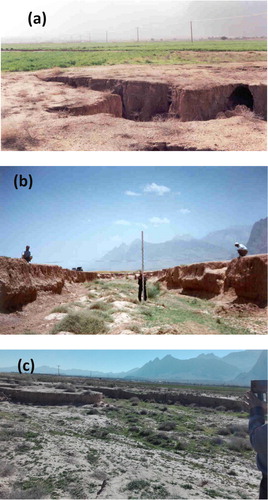
Fareghan watershed is located in Hormozgan province, south of Iran extending between 56° 09′ − 56° 18′ E longitude and 55° 27′ − 32° 22′ 19" N latitude and cover an area of 138 ${\mathrm{km}}^2$ (Figure 1). Minimum and Maximum of watershed elevation were 1074 and 3117 m.a.s.l., respectively. The study area receives an average annual rainfall of 219.7 mm, and ranged from 67.4 till 568.5 mm. Most of the rainfall occurs in winter. The annual average temperature, minimum annual average temperature and maximum annual average temperature are 26.2 °C, 21.6 °C and 30.8 °C, respectively. Climate is classified as dry hot and very dry hot. Soil texture is Silt-Loam in plant covered sites and are silty-clay and clay in the eroded bare lands. The surface horizon has the highest degree of salinity. The watershed is geologically most covered by Bakhtiai (most include conglomerate and calcareous sandstone) and Mishan (include marls and clay limestones) formations. The expansion of Gully in this study identified in the Mishan formations and valley terrace and low-level piedmont fan. Image of gully erosion showed in Figure 2. In order to study the geometric features and physical and chemical properties of the soil, 20 ditches as sediment collectors were sampled in the study area. The expansion of gullies takes place in agricultural land located in the pediment area. The ditches are claw-shaped, and their cross-sectional shape is U-shaped. The average depth, width and head-cut width were 2.24, 12.7 and 1.35 m, respectively . To evaluate the soil characteristics of the gully area, it has been applied laboratory measurements. Soil samples were collected until a depth of 290 cm and transported to the laboratory. The Na, Ca and Mg were measured by flame atomic emission spectroscopy, pH was measured using a pH-meter. Measurements of soil EC were collected using an EM38 soil electrical conductivity meter. After the soil particle sizes are obtained, all soil particles are classified into three groups (clay, silt, sand) according to the soil classification system. Soil sampling were selected in 20 gullies a six soil depths: 0–30, 30–75, 75–130, 130–180, 180–250, and 250–290 cm. Soil chemical properties were determined: pH, Electrical conductivity (EC (mmhos/cm)), Na (Meq/lit), Ca + Mg (Meq/lit), Sodium Absorbtion Ratio (SAR), Clay (%), Silt (%), Sand (%).

Figure 1. Location of the study area in Fareghan watershed, Hormozgan province, Iran, as representative of the hot and dry climatic conditions. Source: Author.

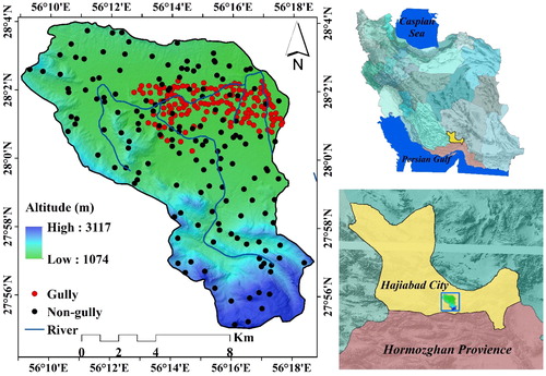
Figure 2. View of the gully erosion in the Fareghan watershed: (a) gully erosion in agriculture area, (b) measurement of morphometric characteristics of gully erosion, and (c) gully erosion in rangeland area.Source: Author.

2.2. Methodology

The head-cut gully erosion locations were based on a field survey developed since 2019/07/22 till 2019/08/6 The head-cut gully were mapped using a Global Positioning System GPS (Garmin GPSMAP 76CSx), which determined a total of 145 erosion points in the study area. In order to determine the non-head-cut gully points, ArcGIS 10.5 software was used, and 145 non-head-cut gully points were randomly selected. Data for modelling were divided within two categories: training and validation, so that 70% of the data was used for training and 30% for the validation sections (Avand et al. 2019; Azareh et al. 2019; Choubin et al. 2019; Moradi et al. 2019; Nhu et al. 2020).

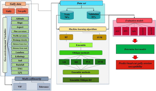
The overview of the head-cut gully erosion susceptibility modelling related to SVM, RF and ensemble Random forest with oblique decision trees has been summarized in a flowchart presented in Figure 3.

Figure 3. Methodological flow chart. Source: Author.

2.3. Dataset preparation for spatial modelling

A total of 145 ground control points (GCP) and none erosion points were collected to survey the generated map by using GIS. According to the process of head-cut gully erosion is affected by climatic, soil features and several environmental variables affecting on head-cut gully erosion be considered. Based on pervious researches (Avand et al. 2019; Lei et al. 2020), 14 variables affecting the head-cut gully erosion susceptibility were selected: altitude, slope, aspect, plan curvature, profile curvature, drainage density, distance from river, distance from road, land use, soil, lithology, rainfall, Stream Power Index (SPI), and Topographic Wetness Index (TWI) were used (Figure 4).

Figure 4. Head-cut gully erosion conditioning factors: (a) altitude, (b) slope, (c) aspect, (d) plan curvature, (e) profile curvature, (f) drainage density, (g) distance from river, (h) distance from road, (i) land use, (j) soil, (k) lithology, (l) rainfall, (m) SPI, and (n) TWI. Source: Author.

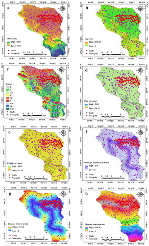
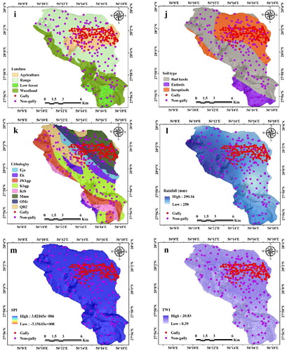
A pixel size of 12.5 m was used for preparing the Digital Elevation Model (DEM) map through ALOSPALSAR sensors (https://search.asf.alaska.edu/#/). The maps of altitude (m), slope (percent), aspect, plan curvature (100/m), profile curvatures (100/m) in the GIS were prepared based on DEM. The surfaces characterized such as slope and altitudinal variability in climate, vegetation, and topography whole the catchment integrated over time caused to imposing altitudinal gradients in precipitation, temperature and hill slope form (Reiners et al 2003). This process ultimately influenced on erosion (Montgomery and Brandon 2002). The slope angle is also regarded as an essential predisposing factor controlling surface runoff, separating of soil particles, and the drainage intensity (Valentin et al. 2005).

The slope aspect is an essential factor for gully erosion that influences climatic characteristics such as precipitation, snow meltwater, land cover, soil moisture patterns, and physiographic trends and hence can be effective on hydrologic conditions (Poiraud 2014; Meinhardt et al. 2015). It appears necessity factor to discover the preparing susceptibility of an area to gully erosion (Umar et al. 2014) because of it can be control the evapotranspiration, vegetation cover, and solar radiation in an area (Sidle and Ochiai 2007; Wang et al. 2011).

Plan curvature determines the maximum slope in a perpendicular direction. It has demonstrated the convergence and divergence of water flow in the ground surface that positive and negative values represented the divergence and convergence of water flow in the study area, respectively. Profile curvature is equal condition to the maximum slope in a specific direction and computed as the slope perpendicular to the slope gradient and has negative and positive values. In contrast, negative and positive values in profile curvature reflect convexity (increasing flow velocity) and concavity (reducing flow velocity), respectively (Jenness 2013). The plan and profile of curvature (100/m) were developed from the DEM with the assistance of ArcGIS 10.5. The map of topography was generated based on wetness index (TWI)) and stream power index (SPI) in SAGAGIS software. TWI determines the effect of topographical factor which describes the distribution of the soil water content and its location relevant to soil situation of the area. Equations (1)(1) $$\mathit{TWI}=In\mathrm{ }\left(\frac{A_s}{\hspace{0.17em}\text{tan}\hspace{0.17em}\beta }\right)$$(1) and (2)(2) $$\mathit{SPI}=A_s\times \hspace{0.17em}\text{tan}\hspace{0.17em}\beta$$(2) were applied to calculate TWI and SPI factors (Moore et al. 1991;  Costache et al. 2020a). (1) $$\mathit{TWI}=In\mathrm{ }\left(\frac{A_s}{\hspace{0.17em}\text{tan}\hspace{0.17em}\beta }\right)$$(1) (2) $$\mathit{SPI}=A_s\times \hspace{0.17em}\text{tan}\hspace{0.17em}\beta$$(2)

Where $A_s$ is the specific catchment area of the basin ($\frac{m^2}{m}$), and$\mathrm{ }\hspace{0.17em}\text{tan}\hspace{0.17em}\beta$ is slope steepness in degrees. The map of distance from stream and road were obtained in GIS software based on the Euclidean extension. Drainages density map was prepared using line density extension to generate raster maps of drainage density and distance to stream. Equation (3)(3) $$DD=\frac{\sum _{i=1}^n{S}_i}{a}$$(3) was applied to calculate drainage density (Horton 1932): (3) $$DD=\frac{\sum _{i=1}^n{S}_i}{a}$$(3)

Where ${\sum }_{i=1}^n{S}_i$ is the total length of drainages in km, and $a$ is the area of the drainage watershed in ${\mathrm{km}}^2.$ The soil map of the study area was obtained based on the map prepared by the Administration of Natural Resources of Hormozgan Province. For preparing the lithology map was used a geological map the National Cartographic Centre of Iran at 1:100,000 scale. Generally, LU/LC map of the watershed was generated based on Landsat 8 images with 30 m spatial resolution, OLI measurement, and the maximum likelihood algorithm in the ENVI 5.5 software, for calculate the NDVI bands 4 (red band) and 5 (infrared band) of OLI imagery in the ENVI 5.5 Software was used. Finally, the annual rainfall map of the study area was prepared depending on the IDW interpolation method in ArcGIS 10.5 based on four synoptic and rain gauges by 30-year period (1989–2019).

2.4. Multi-collinearity analysis

Multi-collinearity is a statistical evaluation tool for the case in which several predisposing factors in a various regression model are robustly correlated, indicating that one can be linearly predicted concerning the others with a non-trivial degree of accuracy (Pourghasemi et al. 2017; Saha 2017). It can be used to remove extremely correlated agents from modelling process and to elude any terminated bias in models’ results. The Tolerance and Variance Inflation Factors (VIF) are two indices that were used generally for reflecting the multi-collinearity of variables (Costache and Tien Bui 2020). These indices determined as follow (Equations (4)(4) $$\mathit{Tolerance}=1-R^{2}J$$(4) and (5)(5) $$\mathit{VIF}=\frac{1}{\mathit{Tolerance}}$$(5) ): (4) $$\mathit{Tolerance}=1-R^{2}J$$(4) (5) $$\mathit{VIF}=\frac{1}{\mathit{Tolerance}}$$(5) where R2J demonstrates the determination of regression coefficient in explanatory variable j on whole the other explanatory variables. A tolerance of >0.10 and variance inflation factors (VIF) >5 illustrate a multi-collinearity problem (Rahmati et al. 2017). The inverse VIF is considered as tolerance where the values <0.1 represent high multi-collinearity (Bui et al. 2011).

2.5. Machine learning method used in modelling the gully erosion

2.5.1. Support vector machine (SVM)

Support vector machine is a discriminative supervised classifier which introduced by Vapnik (1995) in the mid 1990s depending on statistical learning theory. SVM developed as a binary classifier with respect to its efficiency with linearly non-separable and multidimensional data sets (Kavzoglu et al. 2014; Kalantar et al. 2018; Costache 2019). SVM can be applied for both classification and regression purposes (Cristianini and Shawe-Taylor 2000). For this purpose, SVM model used to answer intricate classification and regression problems (Mountrakis et al. 2011). It also reduces the probability of linearity and model over-fitting error and fruitful for processing the data of nonlinear relationships by the kernel function (Naghibi et al. 2016). Kernel function is a one of the most fashionable which called Radial Basic Function (RBF) was applied to address non-linearity of the classification (Pourghasemi et al. 2013; Costache et al. 2020b). For transforming the nonlinear classes into a linear one in high dimensional space was used (Marjanović et al. 2011; Poeppl et al. 2017) following the Equation (6)(6) $$k\left(x,y\right)=\exp (-\gamma {\Vert X_i-X_j\Vert }^2)$$(6) : (6) $$k\left(x,y\right)=\exp (-\gamma {\Vert X_i-X_j\Vert }^2)$$(6) where γ is the gamma parameter. The better the gamma estimate, the better the results.

2.5.2. Random forest (RF)

The random forest algorithm proposed by Breiman (2001) that derived from decision trees (Chen and Liu 2005), that is effective for the data predication and explanation purpose. The random forest algorithm is very popular supervised machine learning technique and make highly accurate classifier (Caruana et al. 2008; Costache et al. 2020c) and incorporates many univariate classification trees to make an ensemble which applied the whole forest as an intricate composite classifier to describe spatial relationship between gully incidence and gully erosion-influencing factors (Breiman 2001; Gayen and Pourghasemi 2019). This approach is appropriate for nonlinear superior dimensional gully erosion evaluation difficulties (Catani et al. 2013; Messenzehl et al. 2017) and can assist to categorize a large number of input variables without bias (Immitzer et al. 2012). For the accomplishment of this model, the user must enter the input number of trees (T) and the number of factors (m) (Pourghasemi and Rahmati 2018). Output of this process with ensemble of trees {Tb}^B1 for new point x as follow as: $$\mathrm{Regression}:\mathrm{ }{f}_{rf}^b\left(x\right)=\frac{1}{b}\mathrm{ }\sum _{b=1}^b{T}_b\left(x\right)$$

Classification: Let C ⁁ b (x) be the class prediction for the both random-forest tree. Then, $C\hspace{0.17em}⁁\hspace{0.17em}\mathit{Brf}(x)\mathrm{ }=\mathrm{ }\mathit{maximum}\mathrm{ }\mathit{vote}\mathrm{ }\{C\hspace{0.17em}⁁\hspace{0.17em}b\mathrm{ }(x)\}\mathrm{ }B1$ (Friedman et al. 2000; Naghibi et al. 2016).

2.5.3. Oblique Random forest (oblique RF)

The oblique RF approach assigned the algorithm for the standard RF. RF chooses a characteristic for splitting the node in terms of a split criterion, oblique RF accomplishes orthogonal decision tree which commonly learns for an “optimal” feature candidate from the feature subset to split the data related to impurity criteria, specially, the standard oblique RF algorithm employs ridge regression or linear discriminative models, rather than using random coefficients as the original oRF. (Marquardt and Snee 1975; Renard 1997) as split model. Furthermore, unlike the original RF implementation, oRF scales included zero mean and unit variance that caused the variables to improve model stability. Splits may bring up the models for the node, (i) class label information only (logistic regression and linear discriminant analysis (LDA)); (ii) data variation (principal component analysis (PCA)); or (iii) an optimum between class label correlation and data (logistic regression, ridge regression, partial least squares (PLS), and SVM).

In the present study, we reviewed classifier based oblique RF (i) logistic regression, (ii) ridge regression, (iii) PLS, and (iv) SVM for multivariate node splitting. Ridge regression intends to gain strength the regression coefficient determination and diminish the variance among highly correlated bands and it is hoped that the net effect will be to give estimates that are more reliable by exerting a penalty on the coefficients (Equation (7)(7) $$\mathit{RSS}\left(\lambda \right)=\sum i=1n(yi-y\hspace{0.17em}⁁\hspace{0.17em}\hspace{0.17em}i)2+\lambda \sum j=1p\beta 2j$$(7) ): (7) $$\mathit{RSS}\left(\lambda \right)=\sum i=1n(yi-y\hspace{0.17em}⁁\hspace{0.17em}\hspace{0.17em}i)2+\lambda \sum j=1p\beta 2j$$(7)

where λ controls the shrinkage of the regression coefficients, n is the number of samples, y is class label, $y\hspace{0.17em}⁁\hspace{0.17em}\hspace{0.17em}i$ is the regression prediction, p is the number of bands, and βj is the j_th regression coefficient.

PLS idea is simple—reduces the dimensionality of a dataset, while maintaining as much ‘variability’ (i.e., statistical information) as possible. PLS computes a set of weights and loadings for a set of factors that is applied to model increasing interpretability but at the same time minimizing information loss, as well as variance among the bands and the classes. These weights and loadings are further implied to calculate the cumulative significance (B-value) of each band; the higher the B-value, the higher the band importance (Equation (8)(8) $$\mathrm{B}\mathrm{ }=\mathrm{ }\mathrm{w}\left(\mathrm{p}\prime \mathrm{w}\right)-1\mathrm{q}\prime$$(8) ) (Mantas et al. 2019). (8) $$\mathrm{B}\mathrm{ }=\mathrm{ }\mathrm{w}\left(\mathrm{p}\prime \mathrm{w}\right)-1\mathrm{q}\prime$$(8) where B is the cumulative gully erosion susceptibility significance, w, p, and q are the band weight, loading, and class weight, respectively.

2.6. Methods of validation and accuracy assessment

The five models namely ROC, AUC, sensitivity, specificity, positive predictive value (PPV), and negative predictive value (NPV) were objectively compared to characterize the most effective approach. The models were validated employing the receiver operating characteristic (ROC) curves (a graphical plot which controls the model performance in a diagnostic test) (Golkarian et al. 2018) and by calculating the area under the ROC curve (AUC) for each model (Chen et al. 2017; Chen et al. 2019, 2020; Costache et al. 2020; Yariyan et al. 2020). It determines the ability of the model to correctly forecast the non-occurrence of a predefined event (Yesilnacar and Topal 2005). The AUC ranges are between 0.5 and 1 which can be classified as follows: 0.5–0.6 (poor), 0.6–0.7 (moderate), 0.7–0.8 (good), 0.8–0.9 (very good), and 0.9–1 (excellent) (Yesilnacar and Topal 2005; Arabameri, Pradhan, & Rezaei 2019a; Zabihi et al. 2019).

Sensitivity, specificity, PPV and NPV, totally recognized as test characteristics which are significant methods to represent the utility of diagnostic tests. Sensitivity and specificity are appointed for a specific type of test. PPV and NPV for a specific type of test belong to the prevalence of a condition in a population. Sensitivity and specificity can be demonstrated in variety of ways, typically such as sensitivity and specificity being the ability of a screening test to discover a true positive and negative, being related to the true positive and negative rate, representing a test’s ability to properly recognize all occurrence and non-occurrence who have and do not have a condition. PPV and NPV are the probability that following a positive and negative test result, that individual will truly have and will not have that specific condition, respectively. Calculating to these diagnostic tests as follows (Equations (9)–(12)): (9) $$\mathit{Sensitivity}=⌈\frac{a}{a+c}⌉\times 100$$(9) (10) $$\mathit{Specifity}=⌈\frac{d}{b+d}⌉\times 100$$(10) (11) $$\mathit{PPV}=⌈\frac{a}{a+b}⌉\times 100$$(11) (12) $$\mathit{NPV}=⌈\frac{d}{c+d}⌉\times 100$$(12)

Where a,b,c and d are true positive, false positive, false negative, and true negative, respectively. The result of the screen test categorized in Table 1 as follows:

Table 1. Result of the screen test based on deriving sensitivity, specificity, and positive and negative predictive values (Banoo et al. 2007).

	Has the condition	Does not the condition
Positve	a True positive	b False positive	Row entries for determining PPV
Negative	c False negative	d True negative	Row entries for determining NPV
	Columns entries for determining sensitivity	Columns entries for determining specificity

3. Results

3.1. Physical and chemical properties

The laboratory analyses and the statistics of whole physical and chemical properties experimental results is illustrated in Table 2. The soil texture from (0–130 cm), (180–250 cm) and (250–290) are Silt-Loam, Sand-Loam and Silt-Loam, respectively. Overall, the main soil texture regarded as Silt-Loam in the Fareghan watershed.

Table 2. Physical and chemical properties of soil in the gullies of Fareghan watershed.

Features	Soil depth (cm)
	0–30	30–75	75–130	130–180	180–250	250–290
PH	7.9	8.2	8.1	8.4	7.7	7.9
EC (mmhos/cm)	67.3	35.1	29.6	55	61.7	49.6
Na (Meq/lit)	434	211	185	397	419	220
Ca + Mg (Meq/lit)	200	126	100	150	160	230
SAR	43.39	26.57	26.16	45.83	46.83	20.512
Clay (%)	72	70	64	62	17	72
Silt (%)	19	17	35	33	80	21
Sand (%)	9	13	1	5	3	7
Soil texture	Silt-Loam	Silt-Loam	Silt-Loam	Silt-Loam	Sand-Loam	Silt-Loam

3.2. Multi-colinearity (MC) analysis

The MC test result (Table 3) shows that all 14 variables used to model the susceptibility to head-cut gulley erosion do not have such a multi-collinearity problem as all have VIF < 5 and Tolerance > 0.1. They are all independent variables and ready for use in the simulation of susceptibility by SVM, RF and Oblique RF.

Table 3. Multi-colinearity analysis to determine the linearity of the independent variables.

Variables	VIF	Tolerance
Altitude	4.11	0.24
Slope	2.98	0.34
Aspect	1.08	0.93
Plan curvature	3.12	0.32
Profile curvature	1.96	0.51
Distance from river	2.94	0.34
Drainage density	2.44	0.41
Distance from road	3.05	0.33
Rainfall	2.23	0.45
Land use	3.91	0.26
Lithology	1.19	0.84
Soil	2.13	0.47
TPI	1.08	0.93
TWI	1.31	0.76

3.3. Head-cut gully erosion susceptibility (HCGES) modelling

The SVM, RF and Oblique RF machine learning models are applied using those 14 independent variables to prepare the HCGES maps. Total three maps have been generated one for each model which is classified into five susceptibility categories like very low, low, moderate, high and very high (Figure 5). From these three maps, it is evident that the central-north-eastern part of the Farghan watershed is much susceptible for head cut gulley erosion. From central part an eastward long corridor of moderate to very high susceptibility zones exist in this region. Apart from this, entire watershed has very low susceptibility to head-cut gulley erosion specially the southern and north-western part of the region (Figure 4).

Figure 5. Head-cut gully erosion map using the five models: SVM, RF, and Oblique RF. Source: Author.

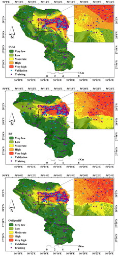
As per the results of HCGES modelling (Table 4), in the very high susceptibility category, RF model has shown the maximum area (14.32 km² or 10.36%) followed by SVM (8.95%) and Oblique RF (8.73%). Similar kind of result is also seen in case of very low susceptibility zone, where RF has predicted highest area (63.15%) followed by Oblique RF (60.24%) and SVM (50.48%). In other three categories like low, moderate and high susceptibility, SVM model has depicted maximum area (24.08%, 8.95% and 7.53%, respectively). These three models have presented more or less similar kind of result with slight variations in areal coverage and spatial distributions.

Table 4. Head-cut gully susceptibility classes’ area.

Models	Area	Susceptibility class
		Very low	Low	Moderate	High	Very high
SVM	Km^2	69.74	33.27	12.37	10.41	12.37
	%	50.48	24.08	8.95	7.53	8.95
RF	Km^2	87.25	22.63	7.13	6.83	14.32
	%	63.15	16.38	5.16	4.94	10.36
Oblique RF	Km^2	83.23	25.66	7.87	9.34	12.06
	%	60.24	18.57	5.70	6.76	8.73

3.4. Validation of the models

The HCGES maps produced by SVM, RF, and Oblique RF are validated by the AUC of the ROC curve method using both training and testing datasets (Table 5 and Figure 6). As per the training datasets, AUC values of SVM and RF are 0.95 and 0.98, respectively. In case of Oblique RF, logistic regression, ridge regression, PLS, SVM and ensemble models have AUC values of 0.99 for each. It means the models are quite accurate in predicting the HCGES zones. The sensitivity or True Positive Rate (TPR) metric values of all the models are >0.9 which implies that the regions identified as head cut gulley erosion prone regions are much accurate. On the contrary, the specificity or True Negative Rate (TNR) numbers are also >0.9 that suggests that the nonerosion prone zones are also very high much correct. The PPV and NPV metric results are also >0.9 for all the models which indicates the robustness of these models. Therefore, validation results from the training datasets have produced splendid positive output in favour of these three models.

Figure 6. The ROC curve analysis for five head-cut gully erosion models using the testing dataset. Source: Author.

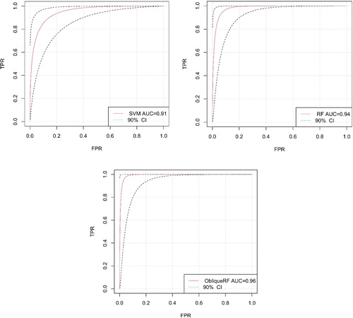
Table 5. Predictive capability of head-cut gully erosion models using train and test dataset.

Models		Stage	Parameters
			Sensitivity	Specificity	PPV	NPV	AUC
SVM		Train	0.93	0.91	0.92	0.91	0.95
		Validation	0.87	0.90	0.89	0.88	0.91
RF		Train	0.98	0.94	0.95	0.98	0.98
		Validation	0.96	0.88	0.88	0.96	0.94
Oblique RF	Logistic Regression	Train	0.99	0.96	0.96	0.99	0.99
		Validation	0.97	0.90	0.90	0.97	0.947
	Ridge Regression	Train	0.99	0.96	0.96	0.99	0.99
		Validation	0.97	0.90	0.90	0.97	0.954
	PLS	Train	0.99	0.96	0.96	0.99	0.99
		Validation	0.97	0.90	0.90	0.97	0.952
	SVM	Train	0.99	0.96	0.96	0.99	0.99
		Validation	0.97	0.90	0.90	0.97	0.946
	Ensemble	Train	0.99	0.96	0.96	0.99	0.99
		Validation	0.97	0.90	0.90	0.97	0.96

Now, based on the testing datasets the AUC values of SVM, RF and Oblique RF are 0.91, 0.94 and 0.96, respectively (Table 6 and Figure 5). It denotes very strong predictive capability of these three models. The sensitivity values are more than 0.9 for all the models except SVM which is 0.87 which implies very good to excellent prediction of susceptible zones. The specificity values of SVM, RF and Oblique RF are 0.90, 0.88 and 0.90, respectively that also suggests very good to excellent prediction of non-susceptible zones. The PPV and NPV values of these three models range in between 0.88 and 0.97 which indicates these models are much robust. Therefore, the validation metrics have shown that all these three models are much accurate and robust in predicting the HCGES zones.

Table 6. Variable importance analysis in RF, oRF, and SVM models for HGES modelling.

Variables	RF	Oblique RF	SVM
Altitude	100	100	100
Aspect	0.02	2.19	1.53
Slope	25.21	25.94	46.021
Plane curvature	2.36	13.2	7.75
Profile curvature	0	0	7.15
Drainage density	14.89	12.89	32.3
Distance from river	20.68	14.39	40.85
Distance from road	61.82	63.72	77.83
Land use	36.95	43.83	65.17
Lithology	21.29	15.52	9.65
Soil	43.51	38.09	70.45
Rainfall	15.89	16.96	30.99
SPI	3.53	12.57	0
TWI	4.98	33.94	6.92

3.5. Variable importance analysis

Fourteen HCGES variables like altitude, aspect, slope, plan curvature, profile curvature, drainage density, distance from river, distance from road, land use, lithology, soil, rainfall, SPI and TWI have been considered for modelling. As per the MC test, all these variables have been identified as independent variables. Now, which of these variables have maximum importance on the susceptibility modelling has been calculated using variable importance analysis of SVM, RF and Oblique RF models (Table 6). According to the results, altitude (100 for each model) has been depicted as the most important variable followed by distance from road (RF = 61.82, Oblique RF = 63.72 and SVM = 77.83). Other important variables are soil, land use, slope, distance from river, rainfall and drainage density (Table 4). As per the RF and Oblique RF models, profile curvature has no role to play in the modelling whereas according to SVM model, SPI has no such importance. Aspect (RF = 0.02, Oblique RF = 2.19 and SVM = 1.53) and plan curvature (RF = 2.36, Oblique RF = 13.2 and SVM = 7.75) are much insignificant factors in gulley modelling and as per RF and SVM, TWI (RF = 4.98 and SVM = 6.92) has also less importance.

4. Discussion

Gully erosion is a significant hydro-geomorphological phenomenon that leads to land degradation and soil loss (Rengers and Tucker 2015; Allen et al. 2018; Hosseinalizadeh et al. 2019). Increased gully erosion in any location can result in the geo-environmental degradation of that region which can affect the life and livelihood of the local people (Jahantigh and Pessarakli 2011; Hassen and Bantider 2020). The precise prediction of gully erosion susceptible zones is therefore much required to implement protection measures. The continuous development of gully erosion modeling with increased accuracy has now become one of the key areas of applied hydro-geomorphological research (Poesen et al. 1998; Hessel and van Asch 2003; Souchère et al. 2003; Arabameri and Pourghasemi 2019). Presently application of machine learning based techniques is in practice which is able to detect the gully erosion prone zones quite accurately (Arabameri et al. 2019; Arabameri et al. 2019; Hosseinalizadeh et al. 2020). Arabameri et al. (2019a) has used Rotational Forest, ADTree, Random Forest, ensemble of Bagging and Logistic Regression to predict the gully erosion in Iran where they have recommended to use Bagging-ADTree model in gully erosion study. Gayen and Pourghasemi (2019) have shown the spatial modelling of gully erosion through CART (classification and regression tree), GLM (general linear model) and CART-GLM models where CART model has the best accuracy level. Arabameri et al. (2019a) have applied Alternating Decision Tree (ADTree), Naïve-Bayes tree (NBTree), and Logistic Model Tree (LMT) for gully erosion modelling where LMT model has performed better than the others. Saha et al. (2020) have used Random Forest (RF), Gradient Boosted Regression Tree (GBRT), Naïve Bayes Tree (NBT), and Tree Ensemble (TE) for this purpose and concluded that RF is best suited for this purpose. Rahmati et al. (2017) has applied RF, SVM, BP-ANN, BRT and others to model the gully erosion susceptible zones where RF and RBF-SVM have produced most accurate result. Therefore, it is seen that classification tree-based methods with ensembles have better accuracy that the conventional machine learning models. Hence, in this study, considering various applications of machine learning based techniques in gully erosion, three models have been utilized like SVM, RF and Oblique RF. All of them have performed very well but among them the Oblique RF model has been shown to be the best model in predicting the HCGES zones using sensitivity, specificity, PPV, NPV and AUC metrics (Table 6). The Oblique RF model using multivariate node splitting models like logistic regression, ridge regression, PLS, SVM and ensemble have done best in all areas of training and validation data sets. This model is therefore perfectly fit for the gully erosion susceptibility analysis, and its performance rate is also excellent.

The multiclass issue according to its architecture can be better tackled in RF than in SVM. RF usually utilizes the data as they are, but in various linear or non-linear forms, SVM depends heavily more on distance which could be the reason for better performance of RF in compare to SVM. In spite of very good results generated by these two, Oblique RF has become the standout performer in this study. Five node splitting models (logistic regression, ridge regression, PLS, SVM and ensemble) of Oblique RF have performed significantly well. Oblique RF is a novel classification technique that is essentially an upgrade of the RF model (Agjee et al. 2018). This model splits the feature space by means of various hyperplanes which are oblique in nature and can manage the noisy data more precisely (Do et al. 2010; Menze et al. 2011). For that reason, it has better suited for the remote sensing data related spatial prediction. Besides, as this model uses supervised linear kind of models like ridge regression, SVM and others which are already stronger in multivariate node splitting at each node therefore the robustness and accuracy level of the Oblique RF model has gone better (Agjee et al. 2018).

If we compare Figures 3 and 4, then we can see that lower altitude, lesser slope, lesser distance from river, agricultural land and Inceptisol soils are favouring the head cut gulley erosion in this region. On the other hand, higher altitude, greater slope and forested land are restricting it. The highest susceptible zones are found near the lowest altitude conditions here it is near about 1074 m. It suggests that lower elevations are favouring the head cut gully erosion which is also reported by Dickson et al. (2007), Arabameri et al. (2019a, 2019c). In this study, lower slope regions (close to 0) are having high gully erosion susceptibility the same has been found by Arabameri et al. (2019b). The reasons may be lower slope are mainly covered by thick soil with lesser strength which is eroded by the rainfall induced high surface run-off from the upslope (Zabihi et al. 2018). It is also noticed that Inceptisol soil regions have widespread gully and this soil type is found in a wide range of environments characterized with poor soil formation (Palmer 2005). The location of the Inceptisols near the river induce a quick surface wash of the material. Amare et al. (2019) has reported that run-off and sub-surface run-off are one of the main drivers of gully erosion citing examples from ample literatures (Moges and Holden 2008). Distance from road is the second most important variable of head-cut gully erosion here which indicates that anthropogenic interferences in terms of development and construction activity over the land leads to the weakening of soil and then surface run-off erodes it to form gully. It agrees with the findings of Arabameri et al. (2019a) where less than 500 m distance from road has been shown as the most gully erosion prone regions. Now, if we look at the landuse map and HCGES maps then it is noticed that agricultural land areas are in the very high susceptible zone. It suggests that tillage led to soil loosening and made the land suitable for gully erosion. Amare et al. (2019) have depicted that valley bottom gully erosion are majorly associated with grazing land and crop land whereas Boardman (2014) and Boardman et al. (2003) have shown that cultivation is mostly associated with gully erosion in semi-arid climatic region. Soil erosion is highly related to the mismanagement of agricultural land (Cerdà et al. 2020). The non-sustainable practices applied in agricultural land induce also the compaction of the soil, mainly due to the pass of machinery (Moradi et al. 2020). Recent research confirms the need of more research and more investigations. The high erosion rates induce the degradation of the soil and then higher runoff discharge and then the development of rills and gullies in agricultural land (Rodrigo Comino et al. 2018).

Aspect, curvature and SPI are contributing very less in HCGES modelling in this region. The TWI determines soil saturation level which is important for gully erosion but it also does not have that much role to play in this region. Rainfall, lithology and drainage density have been depicted as major drivers of gully erosion by many researchers but in this region these parameters have low to moderate importance on gully erosion (Langendoen et al. 2013; Amare et al. 2019; Arabameri et al. 2019; Arabameri, Pradhan, and Rezaei 2019a). Therefore, it may be stated that although the key drivers of gully erosion are uniform for all regions some factors are more important for a particular region which may be insignificant for the others. So, geo-physical conditions of any region should be examined carefully to assess the gully erosion for that region.

5. Conclusion

Gully erosion is a threat to the sustainability of the many regions of the world as they trigger soil erosion and then land degradation as a consequence of the lowering of soil productivity. Gully development also hampers the economic activities and threat the agriculture productivity and human development. Therefore, proper identification and forecasting of head cut gully erosion zones is much essential for the protection and management of the land resource. The scientific community is working to develop gully erosion prediction using various quantitative techniques. Machine learning models and their ensemble with hybrid meta-classifiers are giving very good result as these are able to overcome the challenges of over-fitting and noise. In this study, three machine learning based models (i.e., SVM, RF and Oblique RF) have been used and all of them have performed accurately. The validation metrics like sensitivity, specificity, PPV, NPV and AUC have shown that all these models are excellent to predict both the gully erosion and non-erosion prone zones with high accuracy and among them Oblique RF has become the best, which is the recommended for future researches. From the case study of Farghan watershed we conclude that selecting suitable variables and coupling machine learning with GIS is the best option for heat cut gullies mapping. The susceptible maps produced by this study will surely help the planners and decision makers for the protection and management of erosion prone zones.

Disclosure statement

No potential conflict of interest was reported by the authors.

Data availability statement

Data sharing is not applicable to this article as no new data were created or analyzed in this study.

Correction Statement

This article has been republished with minor changes. These changes do not impact the academic content of the article.

References

- Agjee NH, Mutanga O, Peerbhay K, Ismail R. 2018. The impact of simulated spectral noise on random forest and oblique random forest classification performance. J Spectrosc. 2018:1–8.
- Allen PM, Arnold JG, Auguste L, White J, Dunbar J. 2018. Application of a simple headcut advance model for gullies. Earth Surf Process Landforms. 43(1):202–217.
- Amare S, Keesstra S, van der Ploeg M, Langendoen E, Steenhuis T, Tilahun S. 2019. Causes and controlling factors of Valley bottom Gullies. Land. 8(9):141.
- Arabameri A, Pourghasemi HR. 2019. Spatial modeling of gully erosion using linear and quadratic discriminant analyses in GIS and R. In: Spatial Modeling in GIS and R for Earth and Environmental Sciences. Amsterdam: Elsevier; pp. 299–321.
- Arabameri A, Pradhan B, Lombardo L. 2019. Comparative assessment using boosted regression trees, binary logistic regression, frequency ratio and numerical risk factor for gully erosion susceptibility modelling. Catena. 183:104223.
- Arabameri A, Pradhan B, Pourghasemi HR, Rezaei K, Kerle N. 2018. Spatial modelling of gully erosion using GIS and R programing: a comparison among three data mining algorithms. Appl Sci. 8(8):1369.
- Arabameri A, Pradhan B, Rezaei K. 2019a. Gully erosion zonation mapping using integrated geographically weighted regression with certainty factor and random forest models in GIS. J Environ Manage. 232:928–942.
- Arabameri A, Pradhan B, Rezaei K. 2019b. Spatial prediction of gully erosion using ALOS PALSAR data and ensemble bivariate and data mining models. Geosci J. 23(4):669–686.
- Arabameri A, Pradhan B, Rezaei K, Conoscenti C. 2019. Gully erosion susceptibility mapping using GIS-based multi-criteria decision analysis techniques. Catena. 180:282–297.
- Arabameri A, Pradhan B, Rezaei K, Lee C-W. 2019. Assessment of landslide susceptibility using statistical- and artificial intelligence-based FR–RF integrated model and multiresolution DEMs. Remote Sens. 11(9): 1–24.
- Arabameri A, Pradhan B, Rezaei K, Yamani M, Pourghasemi HR, Lombardo L. 2018. Spatial modelling of gully erosion using evidential belief function, logistic regression, and a new ensemble of evidential belief function–logistic regression algorithm. Land Degrad Dev. 29(11):4035–4049.
- Arabameri A, Rezaei K, Pourghasemi HR, Lee S, Yamani M. 2018. GIS-based gully erosion susceptibility mapping: a comparison among three data-driven models and AHP knowledge-based technique. Environ Earth Sci. 77(17):1–22.
- Avand M, Janizadeh S, Naghibi SA, Pourghasemi HR, Khosrobeigi BS, Blaschke T. 2019. A comparative assessment of Random Forest and k-nearest neighbor classifiers for gully erosion susceptibility mapping. Water. 11(10):2076.
- Azareh A, Rahmati O, Rafiei-Sardooi E, Sankey JB, Lee S, Shahabi H, Ahmad BB. 2019. Modelling gully-erosion susceptibility in a semi-arid region, Iran: investigation of applicability of certainty factor and maximum entropy models. Sci Total Environ. 655:684–696.
- Banoo S, Bell D, Bossuyt P, Herring A, Mabey D, Poole F, Smith PG, Sriram N, Wongsrichanalai C, Linke R, et al. 2007. Evaluation of diagnostic tests for infectious infections, general principles. Nat Rev Microbiol. 5(S11):S21–S31.
- Beavis SG. 2000. Structural controls on the orientation of erosion gullies in mid-western New South Wales. Australia. Geomorphology. 33(1–2):59–72.
- Berlin MM, Anderson RS. 2007. Modeling of knickpoint retreat on the Roan Plateau, western Colorado. J Geophys Res Earth Surf. 112(F3): 1–16.
- Boardman J. 2014. How old are the gullies (dongas) of the Sneeuberg uplands, Eastern Karoo, South Africa? Catena. 113:79–85.
- Boardman J, Parsons AJ, Holland R, Holmes PJ, Washington R. 2003. Development of badlands and gullies in the Sneeuberg. Great Karoo, South Africa. Catena. 50(2–4):165–184.
- Breiman L. 2001. Random forests. Mach Learn. 45(1):5–32.
- Breiman L. 2001. Random forests machine learning. 45: 5–32.
- Bui DT, Lofman O, Revhaug I, Dick O. 2011. Landslide susceptibility analysis in the Hoa Binh province of Vietnam using statistical index and logistic regression. Nat Hazards. 59(3):1413–1444.
- Bull LJ. 2002. Dryland rivers: hydrology and geomorphology of semi-arid channels. New York: John Wiley & Sons.
- Caruana R, Karampatziakis N, Yessenalina A. 2008. An empirical evaluation of supervised learning in high dimensions. In: Proceedings of the 25th International Conference on Machine Learning, Helsinki, Finland; p. 96–103.
- Catani F, Lagomarsino D, Segoni S, Tofani V. 2013. Landslide susceptibility estimation by random forests technique: sensitivity and scaling issues. Nat Hazards Earth Syst Sci. 13(11):2815–2831.
- Cerdà A, Rodrigo-Comino J, Giménez-Morera A, Keesstra SD. 2017. An economic, perception and biophysical approach to the use of oat straw as mulch in Mediterranean rainfed agriculture land. Ecol Eng. 108:162–171.
- Cerdà A, Rodrigo-Comino J, Yakupoğlu T, Dindaroğlu T, Terol E, Mora-Navarro G, Arabameri A, Radziemska M, Novara A, Kavian A, et al. 2020. Tillage versus no-tillage. Soil properties and hydrology in an organic persimmon farm in Eastern Iberian Peninsula. Water. 12(6):1539.
- Chen W, Chai H, Zhao Z, Wang Q, Hong H. 2016. Landslide susceptibility mapping based on GIS and support vector machine models for the Qianyang County. Environ Earth Sci. 75(6):474.
- Chen W, Hong H, Panahi M, Shahabi H, Wang Y, Shirzadi A, Pirasteh S, Alesheikh AA, Khosravi K, Panahi S, et al. 2019. Spatial prediction of landslide susceptibility using GIS-based data mining techniques of ANFIS with Whale Optimization Algorithm (WOA) and Grey Wolf Optimizer (GWO). Appl Sci. 9(18):3755.
- Chen W, Li Y, Xue W, Shahabi H, Li S, Hong H, Wang X, Bian H, Zhang S, Pradhan B, et al. 2020. Modeling flood susceptibility using data-driven approaches of na{\"\i}ve bayes tree, alternating decision tree, and random forest methods. Sci Total Environ. 701:134979.
- Chen W, Xie X, Wang J, Pradhan B, Hong H, Bui DT, Duan Z, Ma J. 2017. A comparative study of logistic model tree, random forest, and classification and regression tree models for spatial prediction of landslide susceptibility. Catena. 151:147–160.
- Chen X-W, Liu M. 2005. Prediction of protein-protein interactions using random decision forest framework. Bioinformatics. 21(24):4394–4400.
- Choubin B, Rahmati O, Tahmasebipour N, Feizizadeh B, Pourghasemi HR. 2019. Application of fuzzy analytical network process model for analyzing the gully erosion susceptibility. In: Natural hazards GIS-based spatial modeling using data mining techniques. Berlin, Heidelberg: Springer; p. 105–125.
- Conoscenti C, Angileri S, Cappadonia C, Rotigliano E, Agnesi V, Märker M. 2014. Gully erosion susceptibility assessment by means of GIS-based logistic regression: a case of Sicily (Italy). Geomorphology. 204:399–411.
- Costache R, Hong H, Wang Y. 2019. Identification of torrential valleys using GIS and a novel hybrid integration of artificial intelligence, machine learning and bivariate statistics. CATENA. 183:104179
- Costache R, Tien Bui D. 2020. Identification of areas prone to flash-flood phenomena using multiple-criteria decision-making, bivariate statistics, machine learning and their ensembles. Sci. Total Environ. 712:136492 doi:10.1016/j.scitotenv.2019.136492.
- Costache R, Pham Q B, Sharifi E, Linh N T T, Abba SI, Vojtek M, Vojteková J, Nhi P T T, Khoi D N. 2020a. Flash-Flood Susceptibility Assessment Using Multi-Criteria Decision Making and Machine Learning Supported by Remote Sensing and GIS Techniques. Remote Sensing. 12(1):106 doi:10.3390/rs12010106.
- Costache R, Popa M C, Tien Bui D, Diaconu D C, Ciubotaru N, Minea G, Pham Q B. 2020b. Spatial predicting of flood potential areas using novel hybridizations of fuzzy decision-making, bivariate statistics, and machine learning. J. Hydrol. 585:124808 doi:10.1016/j.jhydrol.2020.124808.
- Costache R. 2019. Flash-Flood Potential assessment in the upper and middle sector of Prahova river catchment (Romania). A comparative approach between four hybrid models. Sci. Total Environ. 659:1115–1134. doi:10.1016/j.scitotenv.2018.12.397.
- Costache R, Hong H, Pham Q B. 2020c. Comparative assessment of the flash-flood potential within small mountain catchments using bivariate statistics and their novel hybrid integration with machine learning models. Sci Total Environ. 711:134514 doi:10.1016/j.scitotenv.2019.134514. PMC: 31812401
- Cristianini N, Shawe-Taylor J. 2000. An introduction to support vector machines and other kernel-based learning methods. United Kingdom: Cambridge University Press.
- De Santisteban LM, Casalí J, López JJ. 2006. Assessing soil erosion rates in cultivated areas of Navarre (Spain). Earth Surf Process landforms. Earth Surf Process Landforms. 31(4):487–506.
- Dickson JL, Head JW, Kreslavsky M. 2007. Martian gullies in the southern mid-latitudes of Mars: evidence for climate-controlled formation of young fluvial features based upon local and global topography. Icarus. 188(2):315–323.
- Do T-N, Lenca P, Lallich S, Pham N-K. 2010. Classifying very-high-dimensional data with random forests of oblique decision trees. In: Advances in Knowledge Discovery and Management. Berlin, Heidelberg: Springer; p. 39–55.
- Friedman J, Hastie T, Tibshirani R. 2000. Additive logistic regression: a statistical view of boosting (with discussion and a rejoinder by the authors). Ann Statist. 28(2):337–407.
- Garosi Y, Sheklabadi M, Conoscenti C, Pourghasemi HR, Van Oost K. 2019. Assessing the performance of GIS- based machine learning models with different accuracy measures for determining susceptibility to gully erosion. Sci Total Environ. 664:1117–1132.
- Gayen A, Pourghasemi HR. 2019. Spatial modeling of gully erosion: a new ensemble of CART and GLM data-mining algorithms. In: Spatial Modeling in GIS and R for Earth and Environmental Sciences. Amsterdam: Elsevier; p. 653–669.
- Gayen A, Pourghasemi HR, Saha S, Keesstra S, Bai S. 2019. Gully erosion susceptibility assessment and management of hazard-prone areas in India using different machine learning algorithms. Sci Total Environ. 668:124–138.
- Golkarian A, Naghibi SA, Kalantar B, Pradhan B. 2018. Groundwater potential mapping using C5.0, random forest, and multivariate adaptive regression spline models in GIS. Environ Monit Assess. 190(3):149.
- Hassen G, Bantider A. 2020. Assessment of drivers and dynamics of gully erosion in case of Tabota Koromo and Koromo Danshe watersheds. Geoenviron Disasters. 7(1):1–13.
- Hessel R, van Asch T. 2003. Modelling gully erosion for a small catchment on the Chinese Loess Plateau. Catena. 54(1–2):131–146.
- Horton RE. 1932. Drainage-basin characteristics. Trans Agu. 13(1):350–361.
- Hosseinalizadeh M, Alinejad M, Behbahani AM, Khormali F, Kariminejad N, Pourghasemi HR. 2020. A review on the gully erosion and land degradation in Iran. In: Gully erosion studies from India surrounding regions. Berlin, Heidelberg: Springer; p. 393–403.
- Hosseinalizadeh M, Kariminejad N, Chen W, Pourghasemi HR, Alinejad M, Mohammadian Behbahani A, Tiefenbacher JP. 2019. Spatial modelling of gully headcuts using UAV data and four best-first decision classifier ensembles (BFTree, Bag-BFTree, RS-BFTree, and RF-BFTree). Geomorphology. 329:184–193.
- Immitzer M, Atzberger C, Koukal T, Osterreich W. 2012. Eignung von WorldView-2 Satellitenbildern für die Baumartenklassifizierung unter besonderer Berücksichtigung der vier neuen Spektralkanäle. Photogramm Fernerkun. 2012:573–588.
- Jahantigh M, Pessarakli M. 2011. Causes and effects of gully erosion on agricultural lands and the environment. Commun Soil Sci Plant Anal. 42(18):2250–2255.
- Jenness J. 2013. Dem surface tools for ARCGIS.
- Kalantar B, Pradhan B, Naghibi SA, Motevalli A, Mansor S. 2018. Assessment of the effects of training data selection on the landslide susceptibility mapping: a comparison between support vector machine (SVM), logistic regression (LR) and artificial neural networks (ANN). Geomatics Nat Hazards Risk. 9(1):49–69.
- Karydas C, Panagos P. 2020. Towards an assessment of the ephemeral gully erosion potential in Greece using google. Earth Water. 12(2):603.
- Kavzoglu T, Sahin EK, Colkesen I. 2014. Landslide susceptibility mapping using GIS-based multi-criteria decision analysis, support vector machines, and logistic regression. Landslides. 11(3):425–439.
- Keesstra S, Mol G, de Leeuw J, Okx J, Molenaar C, de Cleen M, Visser S. 2018. Soil-related sustainable development goals: Four concepts to make land degradation neutrality and restoration work. Land. 7(4):133.
- Keesstra SD, Bouma J, Wallinga J, Tittonell P, Smith P, Cerdà A, Montanarella L, Quinton JN, Pachepsky Y, Van Der Putten WH. 2016. The significance of soils and soil science towards realization of the United Nations Sustainable Development Goals. Soil. 2: 111–128.
- Langendoen EJ, Tebebu TY, Steenhuis TS, Tilahun SA. 2013. Assessing gully widening and its control in the Debra-Mawi watershed, northern Ethiopia. In Proceedings of the First International Conference on Advancement of Science and Technology (ICAST-2013), May 17–18, 2013, Bahir Dar, Ethiop; p. 214–222.
- Lei X, Chen W, Avand M, Janizadeh S, Kariminejad N, Shahabi H, Costache R, Shahabi H, Shirzadi A, Mosavi A. 2020. GIS-based machine learning algorithms for gully erosion susceptibility mapping in a semi-arid region of Iran. Remote Sens. 12(15):2478.
- Luffman I, Nandi A. 2020. Seasonal precipitation variability and gully erosion in Southeastern USA. Water. 12(4):925.
- Malik A, Kumar A. 2018. Comparison of soft-computing and statistical techniques in simulating daily river flow: a case study in India. J Soil Water Conserv. 17(2):192–199.
- Mantas CJ, Castellano JG, Moral-García S, Abellán J. 2019. A comparison of random forest based algorithms: random credal random forest versus oblique random forest. Soft Comput. 23(21):10739–10754.
- Marjanović M, Kovačević M, Bajat B, Voženílek V. 2011. Landslide susceptibility assessment using SVM machine learning algorithm. Eng Geol. 123(3):225–234.
- Marquardt DW, Snee RD. 1975. Ridge regression in practice. Am Stat. 29(1):3–20.
- Meinhardt M, Fink M, Tünschel H. 2015. Landslide susceptibility analysis in central Vietnam based on an incomplete landslide inventory: comparison of a new method to calculate weighting factors by means of bivariate statistics. Geomorphology. 234:80–97.
- Menze BH, Kelm BM, Splitthoff DN, Koethe U, Hamprecht FA. 2011. On oblique random forests. In: Jt European Conference of Machine Learning and Knowledge Discovery in Databases. Berlin, Heidelberg: Springer; p. 453–469.
- Messenzehl K, Meyer H, Otto J-C, Hoffmann T, Dikau R. 2017. Regional-scale controls on the spatial activity of rockfalls (Turtmann Valley, Swiss Alps)—A multivariate modeling approach. Geomorphology. 287:29–45.
- Micheletti N, Foresti L, Robert S, Leuenberger M, Pedrazzini A, Jaboyedoff M, Kanevski M. 2014. Machine learning feature selection methods for landslide susceptibility mapping. Math Geosci. 46(1):33–57.
- Moges A, Holden NM. 2008. Estimating the rate and consequences of gully development, a case study of Umbulo catchment in southern Ethiopia. Land Degrad Dev. 19(5):574–586.
- Montgomery DR, Brandon MT. 2002. Topographic controls on erosion rates in tectonically active mountain ranges. Earth Planet Sci Lett. 201(3–4):481–489.
- Moore ID, Grayson RB, Ladson AR. 1991. Digital terrain modelling: a review of hydrological, geomorphological, and biological applications. Hydrol Process. 5(1):3–30.
- Moradi E, Rodrigo-Comino J, Terol E, Mora-Navarro G, da Silva A, N Daliakopoulos I, Khosravi H, Pulido Fernández M, Cerdà A. 2020. Quantifying soil compaction in Persimmon Orchards Using ISUM (Improved Stock Unearthing Method) and core sampling methods. Agriculture. 10(7):266.
- Moradi HR, Avand MT, Janizadeh S. 2019. landslide susceptibility survey using modeling methods. Amsterdam: Elsevier; p. 259–276.
- Mountrakis G, Im J, Ogole C. 2011. Support vector machines in remote sensing: a review. ISPRS J Photogramm Remote Sens. 66(3):247–259.
- Naghibi SA, Pourghasemi HR, Dixon B. 2016. GIS-based groundwater potential mapping using boosted regression tree, classification and regression tree, and random forest machine learning models in Iran. Environ Monit Assess. 188(1):44.
- Nhu V-H, Thi Ngo P-T, Pham T D, Dou J, Song X, Hoang N-D, Tran D A, Cao D P, Aydilek İ B, Amiri M, et al. 2020. A New Hybrid Firefly–PSO Optimized Random Subspace Tree Intelligence for Torrential Rainfall-Induced Flash Flood Susceptible Mapping. Remote Sensing. 12(17):2688 doi:10.3390/rs12172688.
- Nhu V-H, Janizadeh S, Avand M, Chen W, Farzin M, Omidvar E, Shirzadi A, Shahabi H, J. Clague J, Jaafari A, et al. 2020. Gis-based gully erosion susceptibility mapping: a comparison of computational ensemble data mining models. Appl Sci. 10(6):2039.
- Palmer, A. 2005 Inceptisols. In Encyclopedia of Soils in the Environment, Reference Module in Earth Systems and Environmental Sciences; pp. 248–254.
- Piest RF, Wyatt GM, Bradford JM. 1975. Soil erosion and sediment transport from gullies. J Hydraul Div. 101(1):65–80.
- Poeppl RE, Keesstra SD, Maroulis J. 2017. A conceptual connectivity framework for understanding geomorphic change in human-impacted fluvial systems. Geomorphology. 277:237–250.
- Poesen J, Nachtergaele J, Verstraeten G, Valentin C. 2003. Gully erosion and environmental change: importance and research needs. Catena. 50(2–4):91–133.
- Poesen J, Vandaele K, van Wesemael B. 1998. Gully erosion: importance and model implications. In: Model soil Eros by water. Berlin, Heidelberg: Springer; p. 285–311.
- Poesen J, Vandekerckhove L, Nachtergaele J, Oostwoud WD, Verstraeten G, van Wesemael B. 2002. Gully erosion in dryland environments. In: Bull LJ, Kirkby MJ editors. Dryl rivers hydrol geomorphol semi-arid channels. Chichester, UK: Wiley; p. 229–262.
- Poiraud A. 2014. Landslide susceptibility–certainty mapping by a multi-method approach: a case study in the Tertiary basin of Puy-en-Velay (Massif central, France). Geomorphology. 216:208–224.
- Pourghasemi H, Youse S, Kornejady A, Cerdà A. 2017. Science of the total environment performance assessment of individual and ensemble data-mining techniques for gully erosion modeling. Sci Total Environ. 609:764–775.
- Pourghasemi HR, Jirandeh AG, Pradhan B, Xu C, Gokceoglu C. 2013. Landslide susceptibility mapping using support vector machine and GIS at the Golestan Province. J Earth Syst Sci. 122(2):349–369.
- Pourghasemi HR, Rahmati O. 2018. Prediction of the landslide susceptibility: which algorithm, which precision? Catena. 162:177–192.
- Rahmati O, Haghizadeh A, Pourghasemi HR, Noormohamadi F. 2016. Gully erosion susceptibility mapping: the role of GIS-based bivariate statistical models and their comparison. Nat Hazards. 82(2):1231–1258.
- Rahmati O, Tahmasebipour N, Haghizadeh A, Pourghasemi HR, Feizizadeh B. 2017. Evaluating the influence of geo-environmental factors on gully erosion in a semi-arid region of Iran: an integrated framework. Sci Total Environ. 579:913–927.
- Reiners PW, Ehlers TA, Mitchell SG, Montgomery DR. 2003. Coupled spatial variations in precipitation and long-term erosion rates across the Washington Cascades. Nature. 426(6967):645–647.
- Renard KG. 1997. Predicting soil erosion by water: a guide to conservation planning with the Revised Universal Soil Loss Equation (RUSLE). USA: United States Government Printing.
- Rengers FK, Tucker GE. 2014. Analysis and modeling of gully headcut dynamics, North American high plains. J Geophys Res Earth Surf. 119(5):983–1003.
- Rengers FK, Tucker GE. 2015. The evolution of gully headcut morphology: a case study using terrestrial laser scanning and hydrological monitoring. Earth Surf Process Landforms. 40(10):1304–1317.
- Rodrigo Comino J, Keesstra SD, Cerdà A. 2018. Connectivity assessment in Mediterranean vineyards using improved stock unearthing method, LiDAR and soil erosion field surveys. Earth Surf Process Landforms. 43(10):2193–2206.
- Rodrigo-Comino J, Senciales JM, Cerdà A, Brevik EC. 2018. The multidisciplinary origin of soil geography: a review. Earth-Sci. Rev. 177:114–123.
- Rokach L. 2010. Ensemble-based classifiers. Artif Intell Rev. 33(1–2):1–39.
- Saha S. 2017. Groundwater potential mapping using analytical hierarchical process: a study on Md. Bazar Block of Birbhum District, West Bengal. Spat Inf Res. 25(4):615–626.
- Saha S, Roy J, Arabameri A, Blaschke T, Tien Bui D. 2020. Machine learning-based gully erosion susceptibility mapping: a case study of Eastern India. Sensors. 20(5):1313.
- Sannigrahi S, Chakraborti S, Joshi PK, Keesstra S, Sen S, Paul SK, Kreuter U, Sutton PC, Jha S, Dang KB. 2019. Ecosystem service value assessment of a natural reserve region for strengthening protection and conservation. J Environ Manage. 244:208–227.
- Sidle RC, Ochiai H. 2007. Landslides processes, prediction, and land use. Water Resources Monograph 18. In: Natural Resources Forum. New York: John Wiely and sons; Vol. 31.; p. 322–326.
- Souchère V, Cerdan O, Ludwig B, Le Bissonnais Y, Couturier A, Papy F. 2003. Modelling ephemeral gully erosion in small cultivated catchments. Catena. 50(2–4):489–505.
- Torri D, Borselli L. 2003. Equation for high-rate gully erosion. Catena. 50(2–4):449–467.
- Umar Z, Pradhan B, Ahmad A, Jebur MN, Tehrany MS. 2014. Earthquake induced landslide susceptibility mapping using an integrated ensemble frequency ratio and logistic regression models in West Sumatera Province, Indonesia. Catena. 118:124–135.
- Valentin C, Poesen J, Li Y. 2005. Gully erosion: impacts, factors and control. Catena. 63(2–3):132–153.
- Vapnik VN. 1995. The nature of statistical learning theory. New York: Springer Verlag.
- Visser S, Keesstra S, Maas G, De Cleen M. 2019. Soil as a basis to create enabling conditions for transitions towards sustainable land management as a key to achieve the SDGs by 2030. Sustainability. 11 (23): 6792.
- Wang L, Wei S, Horton R, Shao M. 2011. Effects of vegetation and slope aspect on water budget in the hill and gully region of the Loess Plateau of China. Catena. 87(1):90–100.
- Yang R-M, Zhang G-L, Liu F, Lu Y-Y, Yang F, Yang F, Yang M, Zhao Y-G, Li D-C. 2016. Comparison of boosted regression tree and random forest models for mapping topsoil organic carbon concentration in an alpine ecosystem. Ecol Indic. 60:870–878.
- Yariyan P, Janizadeh S, Van Phong T, Nguyen H D, Costache R, Van Le H, Pham B T, Pradhan B, Tiefenbacher J P. 2020. Improvement of Best First Decision Trees Using Bagging and Dagging Ensembles for Flood Probability Mapping. Water Resour Manage. 34(9):3037–3053. doi:10.1007/s11269-020-02603-7.
- Yesilnacar E, Topal T. 2005. Landslide susceptibility mapping: a comparison of logistic regression and neural networks methods in a medium scale study, Hendek region (Turkey). Eng Geol. 79(3–4):251–266.
- Zabihi M, Mirchooli F, Motevalli A, Darvishan AK, Pourghasemi HR, Zakeri MA, Sadighi F. 2018. Spatial modelling of gully erosion in Mazandaran Province, northern Iran. Catena. 161:1–13.
- Zabihi M, Pourghasemi HR, Motevalli A, Zakeri MA. 2019. Gully erosion modeling using GIS-based data mining techniques in northern Iran: a comparison between boosted regression tree and multivariate adaptive regression spline. In: Natural Hazards GIS-Based Spatial Modeling Using Data Mining Techniques. Berlin, Heidelberg: Springer; p. 1–26.