Can we rely on VIIRS nightlights to estimate the short-term impacts of natural hazards? Evidence from five South East Asian countries

Abstract

This paper utilizes Visible Infrared Imaging Radiometer Suite (VIIRS) nightlights to model damage caused by earthquakes, floods and typhoons in five South East Asian countries (Indonesia, Myanmar, the Philippines, Thailand and Vietnam). For each type of hazard we examine the extent to which there is a difference in nightlight intensity between affected and non-affected cells based on (i) case studies of specific hazards; and (ii) fixed effect regression models akin to the double difference method to determine any effect that the different natural hazards might have had on the nightlight value. The VIIRS data has some shortcomings with regards to noise, seasonality and volatility that we try to correct for with new statistical methods. The results show little to no significance regardless of the methodology used. Possible explanations for the lack of significance could be underlying noise in the nightlight data and measurements or lack of measurements due to cloud cover. Overall, given the lack of consistency in the results, even though efforts were made to decrease volatility and remove noise, we conclude that researchers should be careful when analyzing natural hazard impacts with the help of VIIRS nightlights.

Keywords:

• Remote sensing
• VIIRS
• natural hazard
• earthquake
• typhoon
• flood

1. Introduction

Natural hazards and the damages caused by them has seen an increase in media coverage, partly due to the overall focus on climate and climate change, but also due to the larger economic damages compared to previous decades. The latter point is explained through a growing global population and the increasing economic value in settled places. With this value increase comes a need for updated local data on where people live and the economic activity there. This is particularly true in the wake of a devastating natural hazard when it can be difficult to assess damages quickly and accurately.

Recently, remotely sensed data is often used to assess damages and economic activity. The modelling and measurement of natural hazards has been extensively covered in the literature for different hazard types such as earthquakes (De Groeve, et al. 2008), typhoons (Emanuel 2011) and floods (Wu et al. 2014) to name a few. Additionally, nightlight intensity is a common proxy for economic activity, exemplified through numerous studies such as Henderson et al. (2012), Gillespie et al. (2014), Skoufias et al. (2017), Hodler and Raschky (2014), Michalopoulos and Papaioannou (2013) and World Bank (2017).

Some articles combining different methodologies from the two fields to estimate the extent and economic damage caused by natural hazards have also been published (Strobl 2012, Bertinelli and Strobl 2013, Klomp 2016, Del Valle et al. 2018, Nguyen and Noy 2020). These prior studies have primarily relied on nightlights from the Defense Meteorological Satellite Program (DMSP), which has been discontinued since 2013. At the end of the DMSP, a new, more spatially and temporally detailed data set for nightlights, the Visible Infrared Imaging Radiometer Suite (VIIRS) product from the National Oceanic and Atmospheric Administration (NOAA) has been published. Only a few articles have used this data set for natural hazard damage detection, namely Zhao et al. (2018) who employed it on a number of select case studies and Mohan and Strobl (2017) who show the short term impact of tropical cyclone Pam. More recently one has also seen its use for the Nepal earthquake in 2015 (Gao et al. 2020) and hurricanes Irma and Maria in Puerto Rico (Zhao, Liu, et al. 2020). These latter articles use different statistical techniques based on seasonal and trend decomposition using Loess (STL) to remove elements related to background noise, seasonality and trends that is present in the VIIRS data (Levin 2017, Zhao, Hsu, et al. 2017).

The production of the monthly VIIRS data follows the work of Elvidge et al. (2017), whereas the daily data, more commonly known as the Black Marble data, is produced following the work of Román et al. (2018). Both products have numerous advantages over the DMSP. Firstly, they have a higher resolution, 15 arcseconds by 15 arcseconds (463 metre by equator) compared to 30 arcseconds for the DMSP. Furthermore, the VIIRS data is used to produce both monthly and daily products compared to the annual DMSP data, making it possible to compare shorter temporal effects of natural hazards. Finally, the DMSP data is normalized and capped at an upper bound, whereas the VIIRS data has no upper limit. However, the VIIRS data exhibits a lot more noise than what is found in the DMSP data. Part of this is due to stray light corrections that can lead to negative light values for some time periods. Another problem – particularly in the tropics - is the many days with cloud cover, which is prevalent in both nightlight data sets. As a matter of fact, several months have no days with a cloud free measurement. Despite these shortcomings, both the DMSP and the VIIRS data have shown a strong correlation with local GDP (World Bank 2017, Henderson, Storeygard and Weil 2012, Chen and Nordhaus 2015) and this paper will take advantage of this to use VIIRS data as a proxy for economic activity.

The aim of this paper is to develop a general methodology where we combine the VIIRS and natural hazard damage indices to estimate the economic impact of events at a large temporal and spatial level. Due to the large areas covered and the long time series, we will only use the monthly data as it is not feasible from a computational point of view to conduct the analysis based on daily data. Additionally, we try different methods for removing noise and seasonality from the VIIRS data to make it more robust for estimation use. The models used to construct the damage indices build upon the work done in Skoufias et al. 2017. The novelty compared to prior studies in the area lies primarily in the added temporal and spatial details provided by the VIIRS data. Additionally, whereas prior studies have focussed on selected case studies, the methodology here can be used to assess numerous events across large areas and it also attempts to find a general methodology for assessing and cleaning the VIIRS data. Furthermore, the damage and economic impact estimates are improved by utilizing detailed settlement layers. The use of secondary data to improve recognition of human activity has previously been done in the areas of poverty (Jean, et al. 2016) and urban extent (Baragwanath, et al. 2019). In this study, settlement layers are used to: 1) remove nightlight cells with zero population to reduce the impact that non-inhabited cells could have on the analysis and 2) distinguish between urban and rural areas as the asset exposure of these may be different. The settlement layers included in the analysis are from Worldpop (WorldPop 2013, Worldpop 2016) and CIESIN (Facebook Connectivity Lab and Center for International Earth Science Information Network - CIESIN - Columbia University n.d.). Both data sets are high resolution layers that show population density through a combination of satellite images and census data.

We model damage indices for three hazard types - earthquakes, typhoons and floods – by following the methodology from Skoufias et al. (2017) for the former and the latter and Strobl (2012) for typhoons. The indices are all based on physical and objectively measured data to avoid endogenously determined and/or subjective damage measures. This differs from other common methods used for disaster loss assessment and measuring impact of damage (see for example Charles, et al. 2006), since we do not rely on local data on vulnerability and exposure, but primarily on the physical attributes for damage estimation and nightlights as a proxy for exposure. The main caveat is that local vulnerability is not sufficiently taken into account. The reason being that – to our knowledge - high quality, spatially disaggregated vulnerability data does not exist for our countries. For the indices in this paper, a damage estimate for all points is obtained first, then the estimate is combined with the settlement and nightlight data to weight damage with asset exposure. Finally, two types of analysis are performed on the combined estimate.

The first analysis is a case study for each hazard type, namely typhoon Haiyan, which hit the Philippines in 2013, the 2016 Aceh Earthquake and the 2017 floods in Southern Thailand. All three hazards caused significant local damage and were for the most part spatially and temporally separate from other events. The case studies consist of a simple graph showing the difference in mean nightlight values for the nightlight cells that were hit by the hazard and the cells that were not hit over a period starting 12 months before the hazard and until 12 months after. The second analysis focuses on the national level and hazards that occurred between June 2012 and March 2018. By using panel fixed effect regressions with 12 monthly lags, we investigate any short and medium-term impacts that each hazard type has.

We have chosen five countries in South East Asia as studies due to their general lack of local level economic data and prevalence of different natural hazards: Indonesia, Myanmar, the Philippines, Thailand and Vietnam. These countries represent a large portion of the total GDP, population and area of the region. Furthermore, they experience earthquakes, typhoons and floods to a varying degree, arguably making them ideal countries to use as examples.

Overall, the results do not exhibit much significance for either analysis. Two case studies of typhoons in the Philippines had the strongest results, where one displayed a sharp drop in mean nightlight during the month that Haiyan struck and similarly a sharp drop when Rammasun struck in July 2014. However, the overall volatility in the VIIRS data makes it difficult to confidently draw any conclusions. The issue of noise in the underlying monthly data has been well illustrated in Hu and Yao (2019), where the monthly VIIRS data showed much lower correlation with GDP than annual VIIRS and DMSP data¹. The results were similar even when comparing VIIRS means that had been decomposed using STL.

The fixed effects regressions were similarly inconclusive, as there was little if any significance across hazard types and months. Several methods were tried to correct for the noise causing the volatility: 1) dropping any negative light values, 2) setting any value below a certain threshold to zero (both for absolute and real values), 3) running regressions only for cells with populations above a certain threshold and 4) logaritmic hyberbolic sine transformations of the nightlight values. Despite the attempted corrections, the results were consistently insignificant, which could have several causes such as the inherent noise in the VIIRS data, a large percentile of very small or negative measurements, cloud cover or regression methodology.

2. Materials and methods

2.1. Population data

To accurately capture economic activity through nightlights it is important to identify areas where there are people, hence avoiding stray lights or other sources of light that are not connected to human activity. For example, Baragwanath et al. (2019) used daily MODIS data as a second data source to more corretly identify the extent of urban markets in India. To find areas with human activity, we utilize human settlement layers from two different sources.

For Indonesia, the Philippines and Thailand high resolution settlement layers (HRSL) from Facebook Connectivity Lab and Center for International Earth Science Information Network - CIESIN - Columbia University was used to identify settlements. These layers are produced at a spatial resolution of 1 arcsecond (∼30 metres). The underlying data is based on 2015 and combines census data with satellite images from DigitalGlobe. The population is allocated according to subdivision censuses once settlements have been identified from the satellite images.

The Worldpop datasets have been used to identify settlement areas in Myanmar and Vietnam (WorldPop 2013, Worldpop 2016). These datasets have a spatial gridcell resolution of approximately 100 metres at the equator and estimate the number of persons per square. Estimates are provided for 2010, 2015 and 2020. To ensure similarity with the other countries, we utilize 2015. To construct the population files, national totals have been adjusted to match UN population estimates. The adjustment is performed by using a Random Forest model to construct a weighted population density layer, which is then used as a basis to place the population as closely as possible to its real geographical distribution.

In addition to helping identify areas with economic activity and hence the hazard exposure of an area, the settlement layers will be used to distinguish rural and urban areas based upon population density.

2.2. Nightlights data

The main source used to find and identify areas with economic activity and their exposure to natural hazards will be satellite images of nighttime lights. We utilize these as a proxy due to the highly localized nature of natural hazards and how they affect economic activity within populated areas. In an optimal scenario, one would prefer highly spatially disaggregated economic data, but lacking this, one can use nightlights. This methodology has been used in several papers with significant results (Henderson, Storeygard and Weil 2012, Gillespie, et al. 2014, Hodler and Raschky 2014, Michalopoulos and Papaioannou 2013). Henderson et al. (2012) show that following the Asian financial crisis in the late 1990s one can use nightlights to capture the economic downturn in Indonesia. Furthermore, they show that swings in GDP change can generally be captured. Nevertheless, one must account for factors such as cultural differences in light usage, latitude and gas flares in particular when comparing across countries. This study only performs intra-country comparisons and hence the results are unlikely to be affected by any cross-country differences.

All the previously mentioned studies use a prior iteration of nightlight images, the DMSP satellite images. The approximate cell grid size of these images is 1 by 1 kilometre at the equator (30 arcseconds) and the data provided is annual. In contrast, this study utilizes a newer nightlight data set, the VIIRS Day/Night Band (DNB) provided by The Earth Observations Group (EOG) at NOAA/NCEI. The data is produced following the methodology of Elvidge et al. (2017) and it is provided starting in April 2012 and go till present, making the time series much shorter than the DMSP data which start in 1992 and go through 2013. However, the VIIRS DNB images from EOG are monthly, whereas the DMSP data is annual. Furthermore, the VIIRS images consist of 15 arcseconds grids (463 meters at the equator) compared to the 30 arcseconds of DMSP. However, even though the data used in this study is at this resolution, the underlying data used to construct it are sampled at a resolution of 750 m by 750 m. Hence, any resampling can introduce noise in the re-sampled data. The VIIRS coverage spans from 75 N latitude to 65S around the entire globe, meaning that the entirety of South East Asia is included.

The VIIRS data has also seen usage in the economics and natural hazard literature. Firstly, Chen and Nordhaus (2015) have done an analysis finding promising results for VIIRS as an economic and population indicator, also relative to the DMSP product. Secondly, Zhao et al. (2018) used the underlying NPP-VIIRS DNB Daily Data to analyze selected natural hazards and found that the images were useful for detecting damages and power outages, but that cloud coverage was a major limitation in the assessment. In this paper, we would also have preferred to use the daily data, since the shock caused by a natural hazard usually may last only very shortly, and subsequent aid flowing in over the next days or weeks will lead to an underestimation of both the negative effect of the shock and the positive effect of the aid. However, using the daily data was not computationally feasible as the goal was to study long term effects across large areas, meaning that daily observations would have created billions of data points. This would have made statistical analysis unfeasible for most common access to computing power. More recent research utilizing the VIIRS nightlights also point to the limitation of monthly VIIRS in the detection of GDP and urban markets. Hu and Yao (2019) shows how monthly VIIRS data has very low correlation for low income countries². The overall correlation is significantly better for middle income countries and when utilizing annual, corrected data. Even when using annual mean of monthly data, the results are worse than for annual VIIRS and DMSP.

The nightlight data output consists of two variables: the average light radiance from DNB and the number of cloud free days. In the case of South East Asia – and the tropics in general - one will find months with no cloud free days and hence no radiance measurement. To account for months with no radiance value, we have interpolated between the month before and after. Furthermore, for cells with little light, one often finds negative light values due to airglow contamination (Uprety, et al. 2019). There are also problems with seasonality and noise (Levin 2017, Zhao, Hsu, et al. 2017). There is no established standard for how to interpret and correct these measurements, albeit Gao et al. (2020) and Zhao et al. (2020) have tried to use different methodologies related to trend decompositions to get more consistent values. To try to correct for the negative values and the noise, we used different methodologies. Firstly, we performed a simplified version of the steps described in Gao et al. (2020), where STL was used on the radiance values to decompose them into a seasonal, a trend and a remainder component, with the latter two values being used in our regression analysis. Secondly, assuming that negative values are due to errors or faulty measurements, we experimented by setting any negative values to zero. Finally, assuming that any absolute value below a certain threshold is either too low to be correctly measured or erroneously measured, we set the value to 0. This was done for several different thresholds ranging from 0 and up to 0.5 to try to identify any differences in the pattern.

To provide some further details into the volatility and distribution of the VIIRS data, Figures 1 and 2 show the distribution of VIIRS values below 2³ for all countries and their populated areas and the number of cloud free days per month. Looking at Figure 1, one sees a clustering on both sides of 0, with the bin containing 0 and very small values constituting more than 15 percent. Furthermore, more than 13 percent of the total points have a negative value and 46 percent more have a value between 0 and 0.3, meaning that almost 60 percent of all points have negative or very small values. It should be noted that these are only points that have been identified as being populated, meaning that they should be relatively free of disturbance from non-human sources. Despite this, there are still very small deviations from 0.

Figure 1. VIIRS Value Distribution for VIIRS values below 2. Source: Authors’ estimates based on VIIRS and population layer data (see text for details).

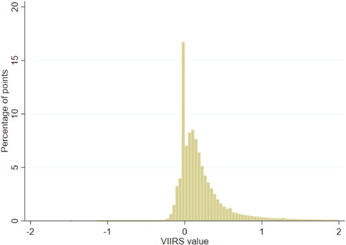
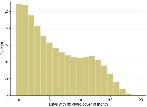
Figure 2. Days with No Cloud Cover in a Month. Source: Authors’ estimates based on VIIRS and population layer data (see text for details).

Even when limiting the light to cells with population over 50 (approximately 30 percent of populated cells), the distribution stays similar with 85 percent of light values being below 2, 75 percent below 1, 46 percent below 0.3 and 5 percent being negative. This distribution pattern follows through to high population numbers. When looking at population numbers above 1,000 (less than 12 percent of the total) 17 percent of the points still have nightlight values below 0.3 albeit only 0.3 percent of points have values below 0. The cause of why the values are so low is not known, but it could be due to the algorithm used to determine the stray light correction. The question will then be if VIIRS is only useful for very urbanized areas, if at all.

Figure 2 provides an overview of the distribution of cloud free days. The first thing of note is that there are no points or months that have more than 20 cloud free days, meaning that no month has used more than 2/3 of the days to get a monthly mean value. The median is 4 days and the mean is 6, and in almost 11 percent of months there were no cloud free days. Overall, the implication is that the monthly values in reality consist of a rather small subsample of the potential days. Additionally, the cloud free days could be clustered towards either end of a month, essentially introducing “noise” in the temporal trend. It might not matter much for a non-climate related hazard such as earthquakes, but for a flood, which is highly correlated with clouds, it might mean that the mean value is based on values before or long after the event has occurred.

2.3. Constructing the damage indices

2.3.1. Earthquakes

To construct damage indices for earthquakes, this paper uses the same methodology as in Skoufias et al. (2017), which in turn is based on damage modelling from contour maps generated by seismological ground stations (GeoHazards International and United Nations Centre for Regional Development 2001, De Groeve, et al. 2008).

In short, these contour maps are ShakeMaps from USGS, which are automatically generated maps providing several key parameters following an earthquake. The parameters peak ground acceleration (PGA), peak ground velocity (PGV) and modified Mercalli intensity (MMI) are used as a base for localized impact. More specifically, the ShakeMaps use data from seismic stations that is interpolated using an algorithm which is similar to kriging. To model the intensity in each coordinate, the model also takes into account ground conditions and the depth of the earthquake. The ShakeMaps are interpolated grids with point coordinates spaced approximately 1.5 kilometres apart (0.0167 degrees). The different measures are largely interchangeable, and in the GeoHazards International and United Nations Centre for Regional Development 2001 report PGA is used to measure damage since PGA, unlike MMI, is an objective measure, implying that MMI is not easy to obtain reliably across the globe. It is assumed that damage starts at a PGA of 3.9 percent of gravity (g).

The construction of the damage index uses two types of data; the intensity data - expressed as PGA - and building inventory data. The building type data stems from the USGS building inventory for earthquake assessment, which provides estimates of the proportions (based on total number of buildings) of building types observed by country; see Jaiswal and Wald (2008). Without any other information available, we use this as an indication of the distribution of building types and mass, but, necessarily, assume that the distribution is homogenous within urban and rural areas. In essence, the building type is a proxy for how vulnerable the countries are to earthquakes.

Damage curves by building type are derived from the curves constructed by the Global Earthquake Safety Initiative (GESI) project; see GeoHazards International and United Nations Centre for Regional Development (2001). We assume that building quality is homogenous across building type and construct eight different damage curves with different quality rating scenarios (ranging from 0 to 7). Initial analysis showed a minor impact depending on the chosen quality, but lacking information we decided to use a mean quality assumption of 4 across the countries.

To model estimated damage caused by a particular earthquake event the data from the ShakeMaps and GESI are used. Then, one identifies the value of peak ground acceleration that each nightlight cell experiences by matching each earthquake point with its nearest nightlight cell. If the cell is further away than 1.5 kilometres or if it experiences shaking (PGA) of less than 0.05 g the value is set to 0. In order to derive a cell i specific earthquake damage index, ED, the following equation is applied: $$E{D}_{i,q,t}=D{R}_{i,k,t}^{pg{a}_{k,q}}\mathrm{ }q=0,\dots ,7$$ where $DR$ is the damage ratio according to the peak ground acceleration, $\mathit{pga},$ and the urban-rural qualification $k$ of cell $i,$ defined for a set of 8 different building quality $q$ categories.

2.3.2. Typhoons

To model typhoons, a damage index from Emanuel (2011) is used. It assumes that a fraction of property is lost or damaged when wind speeds surpass a threshold in a cubic manner.⁴ Formally our damage index is given by: $$f=\frac{v_n^3}{1+\mathrm{ }{v}_n^3}$$ where $f$ is the fraction of property lost or damaged and $v_n$ is: $$v_n\equiv \frac{\mathit{max}\left[V-V_{\mathit{thresh}},\mathrm{ }0\right]}{V_{\mathit{half}}-V_{\mathit{thresh}}}$$ where $V$ is the wind speed, $V_{\mathit{thresh}}$ is the wind speed at and below which no damage occurs (set at 92.6 km/h) and $V_{\mathit{half}}$ is the wind speed at which half the property is destroyed (set at 203.7 km/h).

The wind speed data we use follows Strobl (2012), which in turn is based on a wind field model developed by Boose et al. (2004) and based on Holland (1980). The base equation is given as: $$V_{}=G*F\left[V_m-\mathrm{S}\left(1-\text{sin}\left(T_{}\mathrm{ }\right)\right)\frac{V_h}{2}\mathrm{ }\right]{\left[{\left[\frac{R_m}{R_{}}\right]}^B\hspace{0.17em}\text{exp}\hspace{0.17em}\left(1-{\left[\frac{R_m}{R_{}}\right]}^B\right)\right]}^{1/2}$$ where $V$ is the wind speed at point $P,$ $V_m$ is the maximum sustained wind velocity anywhere in the hurricane, $T$ is the clockwise angle between the forward path of the hurricane and a radial line from the hurricane centre to the point of interest (the centroid of a Parish), $P,$ $V_h$ is the forward velocity of the hurricane, $R_m\mathrm{ }$ is the radial distance from the centre of the hurricane to point $P,$ and $G$ is the gust wind factor (water = 1.2, land = 1.5). Finally, $F$ is a scaling parameter for surface friction (water = 1.0, land = 0.8), $S$ is the asymmetry due to the forward motion of the hurricane (1.0) and $B$ is the shape of the wind profile curve (1.2). These parameter values have been verified in Boose et al. (2001) and Boose et al. (2004).

The source for the localized wind speeds is the IBTrACS database that provides the strength and tracks every 6 hours of all typhoons that affected South East Asia during the period. A potential caveat of using this model is that it has not been validated in terms of the level of vulnerability and exposure one might expect in the countries in this study. This could lead to an under- or overestimation of the damage depending on the local conditions. However, our choice of damage curve used in line with what has been used in the Caribbean, which yielded significant impacts on nightlights (Bertinelli et al. 2016).

2.3.3. Floods

The modelling of floods in this paper is done by using rainfall as a proxy. The daily precipitation data used are from the 3-hourly data set from the Tropical Rainfall Measurement Mission Project (TRMM), which is aggregated up to daily data.⁵ This has been used in several flood related publications before, such as Wu et al. (2012), Wu et al. (2014), Harris et al. (2007), Rahman et al. (2012) and Yuan et al. (2019).

To construct a flood proxy from the TRMM data, we define when a flood event is happening. Both Wu et al. (2012) and Wu et al. (2014) use runoff estimates to define thresholds. However, due to the lack of runoff estimates in our data, we modify their runoff model and define the following flood threshold: $$Ra>P_{95}+\mathrm{\sigma }$$ where $Ra$ is the rainfall in millimetres, $P_{95}$ is the 95th percentile value and $\mathrm{\sigma }$ is the standard deviation of the rainfall.

The flood data set contains daily data, which is aggregated up to monthly values and combined with the nightlight data. When aggregating we constructed two flood proxy variables: 1) A simple count variable that counted number of days that breached the flood threshold. 2) Total rainfall in millimetres above the flood threshold. Overall, this methodology is relatively rudimentary and does not take into account local exposure or vulnerability.

2.4. General empirical strategy

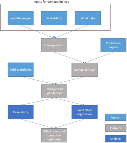
The goal is to analyze the effect that natural hazards might have on the economic activity in an area. To try to correctly identify any such effect, a data set was constructed for each natural hazard type. These sets contain localized nightlight values and damage indices for each hazard type, the total population in each light cell and administrative boundary data linking each nightlight cell to different administrative levels. The general methodology can be seen in Figure 3.

Figure 3. Flow chart for methodology.

The approach we have chosen to construct the data sets is somewhat similar to what was done in Skoufias et al. (2017), where the authors constructed damage indices, weighted with nightlights and aggregated up to annual values at a province or municipality level. However, there are also significant differences between the methods.

Firstly, the nightlight data used as a proxy for economic activity is monthly – and not yearly – providing more accurate temporal data, in particular in the short term. Furthermore, the spatial resolution is much higher, with the VIIRS data providing details down to 450 metre square cells at the equator compared to 1 kilometre squares for the DMSP.

Secondly, by using high resolution population layers to identify areas with economic activity one aims to remove noise from adjacent non-economic areas. By excluding non-inhabited cells, we essentially remove radiance values from stray lights and other non-economic light sources such as forest fires, and one can correctly identify change in nightlight values due to an increase or decrease in economic output. One potential caveat of removing cells with no or very low population numbers is that some agricultural land or assets will not be included in the analysis and hence we might underestimate the damage, especially if these areas are more vulnerable than the areas included in the analysis. However, the assumption is that the asset exposure is closely correlated with how densely populated an area is and that the population density is linked to the radiance values, meaning that the overall damage in low-populated areas is very small compared to densely populated areas. Normally, to be able to set a population threshold one would have to rely on local data, but given the large spatial areas analyzed in this paper, we will run the analysis with several different thresholds to analyze the impact on the final results. In case the results significantly change, we will try to identify a more accurate threshold based on available local data. Finally, instead of aggregating up to a provincial or municipality level, the data is kept at a cell level.

More specifically with regards to the methodology, one starts with localized damage data modelled from actual intensity measures. These values were matched with any intersecting VIIRS cell and assigned to the corresponding month. For light cells that intersected several damage cells a mean value was used. As earthquake damage estimates were modelled based on centroids, only the centroid intersection was used.

Once the nightlight and damage data had been merged, population data was included. The population data sets were aggregated up to the same cell size as the VIIRS data and then matched to find the total population in each nightlight cell. Due to slight differences between the HRSL and Worldpop data sets, two different cut-offs for populated cells were utilized. As HRSL specifically provide settled areas and set other areas to having 0 population, any VIIRS cell with no settled areas in it, would be excluded from the final data set. As for the WorldPop data, any VIIRS cell with less than 5 people in it was considered essentially unpopulated.

Following the construction of the data sets, a simple case study on a large singular event is performed. The case studies are done on the Aceh earthquake in 2016, the Haiyan Typhoon in 2013 and finally for the 2017 floods in Thailand. All these events caused severe damages in the affected areas and one would expect a significant change in nightlight values ex-post.

The Aceh earthquake is the single most damaging event in our study period and occurred in the Indonesian province of Aceh in the morning of 7 December 2016. The magnitude was measured to be 6.5 M_w with 104 fatalities and more than 80,000 displaced. The affected area was rather small, primarily affecting the Pidie Jaya Regency towards the northwestern tip of Sumatra. However, within the Regency it was stated that as much as 30% of the area was affected, making it a highly localized event that caused severe destruction and hence a good case to test for any local area heterogeneity between damaged and non-damaged cells.

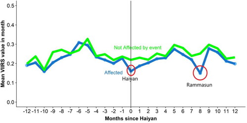
The case study on typhoons is the typhoon Haiyan, also known as typhoon Yolanda, on the Philippines, which was active from November 3 2013 through November 11 2013. It made landfall in the eastern parts of the Philippines on November 7 with wind speeds that were 305 km/h, a then-record velocity. It continued across the middle islands of the Philippines leaving the islands on November 8. It is known as the deadliest and costliest typhoon to hit the Philippines in modern times, killing 6300 people and causing damages worth USD2.2 billion. Furthermore, in July 2014 typhoon Rammasun struck some of the same areas and costing USD885 million in total damages, the third costliest typhoon ever to hit the Philippines.

The third case study are the 2017 Southern Thailand Floods, which happened in the southern parts of Thailand during December 2016 and January 2017. These were the largest floods in over 30 years in these parts of Thailand. Malaysia was also affected, although to a lesser extent. There were almost 100 fatalities and the total costs was USD4 billion, meaning the floods significantly local economies. The reason why these floods were chosen is twofold. Firstly, they lasted only 2 months, unlike the ones in 2013 that lasted approximately 4 months. Secondly, they were isolated compared to other events. The 2014-2015 floods would potentially be capturing the 2013 floods.

To check for any effect from the hazards, we performed a mean comparison of nightlight values between cells that experienced damage and those that did not. Two graphs were constructed for each event; one with the mean of the nightlight values of cells that were struck by the event and one with the cells that were not affected. Furthermore, the analysis focussed on the affected regions – state or province level - and not the national averages.

The second analysis consists of a fixed effects regression for each country and natural hazard type to see if any statistically significant national effects exist. The regressions are lagged for the 12 months following the hazards to allow for any short- and mid-term effects to materialize. The regressions include corrections for time and spatial effects and to correct for potential heteroscedasticity, Driscoll-Kraay standard errors are used (Driscoll and Kraay 1998). The model can be stated as: $$L_{i,t}={\beta }_0+{\mathrm{\Sigma }}_{\mathrm{n}=0}^{12}{\beta }_{\mathrm{n}+1}E{D}_{i,q,t-n}+{\theta }_i+e_{i,t}$$ where $L_{i,t}$ is the light level in cell i in month t and $E{D}_{i,q,t}$ represents the damage or intensity value in the same cell and at the same time. Lags are allowed from month t to t-12. ${\mathrm{\beta }}_0$ is the intercept, ${\mathrm{\theta }}_i$ are the cell fixed effects and $e_{i,t}$ is the error term. In short, it gives the coefficients for the effect that a natural hazard has on the nightlights for the month when the hazard happens and the 12 subsequent months. One should note that the fixed effects ${\mathrm{\theta }}_i$ control for all unspecified time invariant location specific differences, such as geographical features.

3. Results

3.1. Case study results

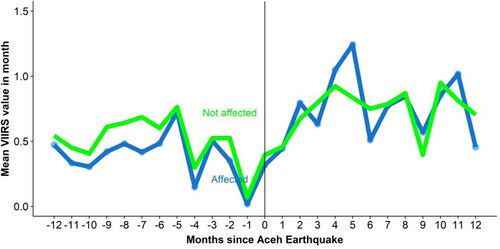
Figures 4 through 6 show the mean VIIRS value for the three case studies for affected and unaffected cells. All figures have a green line depicting the monthly mean radiance value for cells that were not damaged by the hazard in question, while there is also a blue line showing the mean value for cells that were damaged. All graphs start 12 months before the case study occurs and ends 12 months ex-post and the means are calculated for cells within the same administrative boundary. The graphs show the results when comparing the interpolated radiance values. In addition, we did the same analysis with raw radiance values and with STL decompositions where we compared the trend and the remainder means for the two groups of cells. These additional checks did not change the results.

First, Figure 4 shows the results for the case study of the 2016 Aceh Earthquake. The mean values fluctuate and the month before the earthquake the radiance means almost drop to zero. For the months after the earthquake, there is an upward trend, and the affected cells seem to fluctuate more than the non-affected ones. Overall, the two groups exhibit similar trends and fluctuations.

Figure 4. 2016 Aceh Earthquake – Mean of nightlight cell values in the province of Aceh split between cells that were affected by the earthquake and those that were not. Source: Authors’ estimates based on VIIRS and population layer data (see text for details).

Figure 5 depicts the nightlight intensity before and after typhoon Haiyan struck the Philippines. There is less volatility than for the Aceh earthquake and the month of Haiyan shows a clear distinction between damaged cells and those that were not damaged with the former group having a negative drop of approximately 0.05 or 25% of the mean. After the month of Haiyan the radiance value growth in the damaged cells is higher than for the non-damaged group until many of the same cells are struck by typhoon Rammasun 8 months later, when there is another sharp decline in radiance values. However, already the following month, the two groups show similar means.

Figure 5. Case study of Typhoon Haiyan and Rammasun showing the mean VIIRS value for cells that were affected by typhoon Haiyan and those that were in the same province but that were not damaged. Source: Authors’ estimates based on VIIRS and population layer data (see text for details).

Finally, Figure 6 shows the graphs for the 2017 Southern Thailand floods. When using our flood estimator with the rainfall data almost all cells in an area would be affected due to the relatively homogenous rainfall values across large areas. To avoid the problem with a small sample size of non-affected cells a new flood estimator was used. This estimator was set to 1 if the total rainfall in a month above our flood definition exceeded 500 mm. Although this number is somewhat arbitrary, it should capture a select set of especially impacted cells.

Figure 6. 2017 Southern Thailand Floods mean VIIRS nightlight values before and after for impacted and non-impacted cells. Source: Authors’ estimates based on VIIRS and population layer data (see text for details).

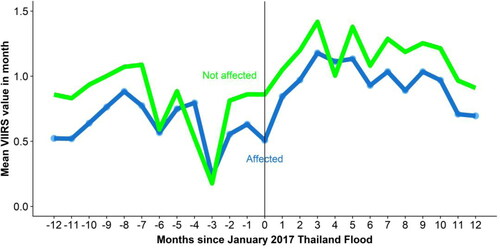
Having imposed the new flood threshold produced the result in Figure 6, which shows the means 12 months before and after January 2017. The flood graphs show a very high level of volatility. However, there is a drop for the most affected cells in the month of the flood, and this do seem to lag below the general trend of the non-affected cells.

3.2. Regression results

Figures 7 through 9 show the fixed effect regression coefficients by country for the earthquakes, typhoons and floods. The regressions were run individually by country and hazard type; thus it is assumed that the impacts from each hazard type is perpendicular to each other. Furthermore, it is assumed that any VIIRS radiance value below 0.3 is 0 and that any cell with fewer than 10 inhabitants is rural.

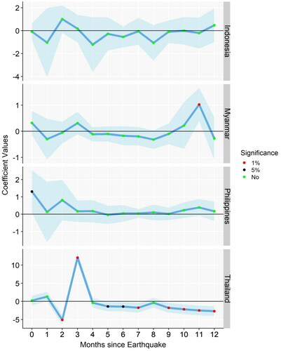
Figure 7 shows the results for the 4 countries that experienced damaging earthquakes during our period. The nightlight radiance values were not impacted in a statistically significant way in Indonesia and Myanmar, except for 11 months ex-post in Myanmar. The Philippines show a positive and significant impact during the month of the earthquake and Thailand a strongly significant and negative impact two months after the earthquake followed by a very strong positive impact in month 3 before a small, but negative and statistically significant, effect for the months 5 through 12. However, Thailand has a small sample of only 169 affected nightlight cells with modest damage.

Figure 7. Earthquake coefficients with 95% confidence intervals. Source: Authors’ estimates based on VIIRS and population layer data (see text for details).

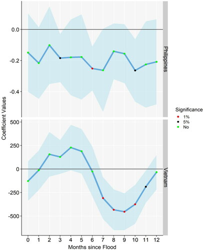
Figure 8 shows the typhoon coefficients for the two affected countries, the Philippines and Vietnam. The Philippines experience a negative and significant effect for months 3, 6 and 10 after a typhoon makes landfall, whereas Vietnam shows a negative and significant effect for months 7 through 11.

Figure 8. Typhoon coefficients with 95% confidence intervals. Source: Authors’ estimates based on VIIRS and population layer data (see text for details).

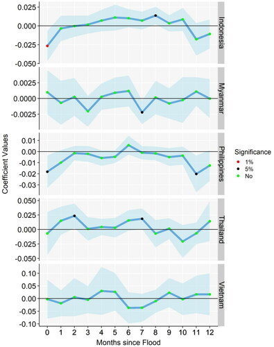
Finally, Figure 9 shows the coefficients associated with flooding for our 5 South East Asian countries. Overall, there are only a few months that are statistically significant. However, we find that for both Indonesia and the Philippines there is a negative and statistically significant effect during the month of the flood, but this effect disappears in the following months. Apart from that, there is a positive impact in month 8 for Indonesia and a negative one in month 11 for the Philippines. The other countries show no strong patterns or effects and only exhibit significance during scattered months, with only month 7 being significant in Myanmar, months 3 and 7 in Thailand and no month being significant in Vietnam.

Figure 9. Flood coefficients with 95% confidence intervals. Source: Authors’ estimates based on VIIRS and population layer data (see text for details).

4. Discussion

Overall, the results in this study showed a general lack of consistency across hazard types and countries. To check if the lack of significant results were due to our assumptions further examinations and robustness checks were performed both for the case studies and the fixed effect regressions.

With previous studies showing promising results when using VIIRS data for earthquakes (Zhao et al. 2018; Gao et al. 2020) and hurricanes (Zhao et al. 2020), one would expect that when one tried to correct for noise and seasonality one could see similar statistically significant results also on a more general scale. Also, given the geographical and cultural similarities between the countries in our sample, one could reasonably expect to see consistent and similar results for each of the different types of hazards. However, despite trying several different correction and transformation methods - both on a case by case basis and generally - the results remained inconsistent and insignificant. For instance, for the Aceh earthquake case we investigated whether there was a particular reason for the general volatility and in particular the sudden decline in radiance values the month before the earthquake. However, apart from finding the value change to be nationwide from November to December, we found no information on other hazards or major power outages during that period. Using STL to decompose into a trend value and a remainder value did not have any impact between the means of the two nightlight cell groups either. The difference between the means were statistically insignificant. When applying the same methods to the 2017 floods in Thailand, we found similar results.

The most likely explanation for these results is some noise or measurement error in the underlying VIIRS data. This is not surprising given the seasonality and noise found in the data (Levin 2017, Zhao, Hsu, et al. 2017). However, it could also potentially be due to aid and relief efforts being deployed quickly and to the correct areas, and hence cancelling out any negative effect on the radiance values of the affected cells. Unfortunately, we lack any geomapped or geographic aid data that could help validate this hypothesis.

The graph for typhoon Haiyan in Figure 5 shows the most consistent radiance values, even though some volatility with spikes and troughs are still present. Most importantly, the graph shows Haiyan’s strong negative effect on nightlight values and a similar drop 8 months later, when Rammasun would strike many of the same cells. Interestingly, one finds a sharp recovery in radiance values in the months following the hazards, potentially due to the influx of aid and personnel. The recovery seems to benefit the areas that were hit by the typhoon the most, implying that the aid reached the areas in need.

For the regressions, which are using nightlight cells from entire countries across a longer temporal period, one needs to make an assumption with regards to the treatment of VIIRS values below or close to 0. Currently, there is no consensus in the literature on how to correct this. The radiance value is set by deducting a dark offset from the raw day/night value. This offset is sometimes severely impacted by airglow leading to negative light values. To correctly account for this, several options were explored. Firstly, the regressions were run with any light value below 0.1 set to 0. Then absolute values were used with any absolute value below thresholds of 0.1, 0.3 and 0.5 set to 0. Irrespective of the chosen threshold, the results did not change in a statistically meaningful way. Given the distribution of the data, with the large majority of cells having values below 0.5, a higher threshold could not be justified as it would clearly exclude radiance values from areas that were populated. Furthermore, given the lack of impact on the results from changing the threshold value, it was decided to not pursue the threshold analysis any further.

When looking at the different hazard types, there was no consistency of results across countries and very few showed any statistically significant impact. For example, in the case of Indonesia, a country that experiences several damaging earthquakes a year, there was no discernable statistical effect either immediately or ex-post. This might be due to several factors. As Indonesia is often struck by earthquakes, they might have efficient methods for dealing with the damage from earthquakes. It could also be that the regression specifications were not suitable for analyzing a country such as Indonesia. Due to the size and geography, there might be large local differences, such as usage of electric light, building methods and quality, and how natural disasters are dealt with. This potential spatial clustering would preferably be controlled for, but it has not been computationally possible to do this due to the dimensional increase of the regression matrix when clustering across multiple regions. Secondly, there might be regional or national differences for when an earthquake is causing damage and hence the PGA threshold for damage might be too low or too high. However, the lack of significance is more likely to have other causes.⁶ It might be due to local cloud cover leading to poor measurement conditions or it could be due to the regression specifications being unable to quantify the relationship. As for the latter point, due to the random nature of earthquakes and the lack of other confounding variables, one would expect that the objective damage variable would accurately estimate the impact meaning that any potential errors are related to either the damage modelling or the VIIRS data. However, to be able to correctly identify the source of the error, one would need to analyze each earthquake event individually, preferably with locally validated damage data, and have access to high-resolution GDP data for comparison and validation against the nightlight data.

Typhoons and floods showed a similar lack of results across countries, with the exception of Indonesia – and to a smaller extent the Philippines - in the month of a flood event. The coefficient on the damage index is strongly negative and significant. The immediate return to insignificance might be an indication that most floods are small, local events where repairs are often carried out almost immediately. However, it is unlikely that the Philippines and Indonesia would be impacted differently from the other 3 countries given the similarities in climate and GDP. Furthermore, the two hazard types are weather related implying that the radiance values are likely to be impacted by significant cloud cover, which are correlated with floods and typhoons.

5. Conclusion

Our findings do not indicate a causal relationship between nightlight values and natural hazard events. Given the lack of consistency in the results despite the efforts to decrease volatility and remove noise, we conclude that researchers should be careful when analyzing natural hazard impacts with the help of VIIRS nightlights. The analysis shows a lack of significance across all hazard types and all countries, despite taking multiple approaches to try to correct for any measurement problems in the data or methodology. The most likely cause for the lack of significant results is the noise and natural volatility in the VIIRS data that is due to measurement precision and cloud cover. Another likely factor is that our sample of low-income countries and the low correlation between monthly VIIRS and GDP is not a good fit for a broad analysis like this. These different factors might also explain why the authors found stronger results using the annual – and in most ways inferior - DMSP data in Skoufias et al. (2017). Finally, it might be that the unique local spatial and cultural attributes make it very difficult to get generalized and significant results.

Nevertheless, the data and the methodology has shown previously that it has merit and use, with this paper simply demonstrating some of the limits of the data and that it is important to consider the temporal and spatial scale of analysis and carefully review both the data and the results to account for factors such as noise, cloud cover, light levels and urbanization. However, the main problem with using the data is that it is difficult to disentangle and quantify the different effects that these factors would have on the radiance values.

An extension of this research for other researchers can be to look at specific cases and see if one could identify effects at a more local scale, preferably with high-resolution and good quality underlying data. With the recent proposed correction methods in Gao et al. (2020) and Zhao et al. (2020) it might also be possible to use STL as a basis to construct a more general methodology for correcting the VIIRS measurements, in particular if it is based on validated GDP data. Additional research efforts could be focussed on different regression methodologies as this type of analysis could lend itself well to other methods. Finally, with the addition of secondary data from other sources such as for example daytime satellite images, vegetation images, national census data or similar one could use machine learning methods to try to account for or correct some of the noise and better identify places of economic activity.

Acknowledgments

This paper was funded by the global knowledge program of the World Bank’s Poverty and Equity Global Practice.

Disclosure statement

No potential competing interest was reported by the authors.

Data availability statement

The data used in this study were derived from the following resources available in the public domain:

These data were derived from the following resources available in the public domain:

Population data:

Worldpop: https://www.worldpop.org/project/categories?id=3

CIESIN: https://ciesin.columbia.edu/data/hrsl/

Nightlights data:

VIIRS: https://eogdata.mines.edu/download_dnb_composites.html

Natural hazards data:

Earthquakes:

USGS Shakemaps: https://earthquake.usgs.gov/earthquakes/search/

Building inventory data: https://pubs.er.usgs.gov/publication/ofr20081160

Typhoons:

IBTrACS: https://www.ncdc.noaa.gov/ibtracs/index.php?name=ib-v4-access

Floods:

TRMM 3B42RT: https://disc.gsfc.nasa.gov/datasets/TRMM_3B42RT_Daily_7/summary

Notes

1 The annual VIIRS data was not used in this study, as it is currently only available for 2 years

2 If one includes all the low income countries, the correlation is negative (-0.02), but it is heavily skewed by the poorest African nations. With the exclusion of the Central African Republic, the correlation improves to 0.12.

3 Values below 2 constitute approximately 95 percent of the total. This was done due to the maximum VIIRS value being 17,699 and hence a density graph would be meaningless going from -1.5 to 17,699. Also, any bin above 2 is very small and would not contribute to the graph

4 Damages are related to wind speed in a cubic manner due to nature of energy dissipation of the hurricane

5 The 3B42RT daily derived product is used in this article

6 The Philippines and Thailand did experience some significance. In the case of the Philippines, one finds a significant and positive effect on the nightlights in the month that the earthquake happens. This might be due to good and efficient local infrastructure and efficient aid work. However, with no further effect later it is not clear what might be causing this early light influx as one would expect aid work to last longer than a couple of weeks. In the case of Thailand, there were only 169 cells that were damaged, and there was little heterogeneity across the cells, potentially impacting the results.

References

- Baragwanath K, Goldblatt R, Hanson G, and, Khandelwal AK. 2019. Detecting urban markets with satellite imagery: An application to India. J Urban Econ. :103173.
- Bertinelli L, Mohan P, Strobl E. 2016. Hurricane damage risk assessment in the Caribbean: An analysis using synthetic hurricane events and nightlight imagery. Ecol Econ. 124:135–144.
- Bertinelli L, Strobl E. 2013. Quantifying the local economic growth impact of hurricane strikes: an analysis from outer space for the Caribbean. J Appl Meteorol Climatol. 52(8):1688–1697.
- Boose ER, Chamberlin KE, Foster DR. 2001. Landscape and regional impacts of hurricanes in new england. Ecol Monogr. 71(1):27–48.
- Boose ER, Serrano MI, Foster DR. 2004. Landscape and regional impacts of hurricanes in Puerto Rico. Ecol Monogr. 74(2):335–352.
- Chen X, Nordhaus W. 2015. A test of the new VIIRS lights data set: population and economic output in Africa. Remote Sens. 7(4):4937–4947.
- De Groeve T, Annunziato A, Gadenz S, Vernaccini L, Erberik A, and T. Yilmaz 2008. Real-time impact estimation of large earthquakes using USGS Shakemaps. In Proceedings of IDRC2008, Davos: Switzerland.
- Del Valle A, Elliott RJR, Strobl E, Tong M. 2018. The short-term economic impact of tropical cyclones: satellite evidence from Guangdong province. EconDisCliCha. 2(3):225–235.
- Driscoll J, Kraay A. 1998. Consistent covariance matrix estimation with spatially dependent panel data. Rev Econ Stat. 80(4):549–560. http://EconPapers.repec.org/RePEc. :tpr:restat:v:80:y:1998:i:4:p:549–560.
- Elvidge CD, Baugh K, Zhizhin M, Hsu FC, Ghosh T. 2017. VIIRS night-time lights. Int J Remote Sens. 38(21):5860–5879.
- Emanuel K. 2011. Global warming effects on U.S. hurricane damage. Wea Climate Soc. 3(4):261–268.
- Facebook Connectivity Lab and Center for International Earth Science Information Network - CIESIN - Columbia University. n.d. High Resolution Settlement Layer (HRSL). Source imagery for HRSL © 2016 DigitalGlobe. Accessed 04 02, 2019. https://ciesin.columbia.edu/data/hrsl/.
- Gao S, Chen Y, Liang L, Gong A. 2020. Post-earthquake night-time light piecewise (PNLP) Pattern based on NPP/VIIRS night-time light data: a case study of the 2015 Nepal earthquake. Remote Sens. 12(12):2009.
- Gillespie TW, Frankenberg E, Chum KF, Thomas D. 2014. Nighttime lights time series of tsunami damage, recovery, and economic metrics in Sumatra, Indonesia. Remote Sens Lett. 5(3):286–294.
- Harris A, Rahman S, Hossain F, Yarborough L, Bagtzoglou A, Easson G. 2007. Satellite-based flood modeling using TRMM-based rainfall products. Sensors (Basel). 7(12):3416–3427. MDPI AG)
- Henderson JV, Storeygard A, Weil DN. 2012. Measuring economic growth from outer space. Am Econ Rev. 102(2):994–1028.
- Hodler R, Raschky PA. 2014. Regional favoritism. Q J Econ. 129(2):995–1033.
- Holland GJ. 1980. An analytic model of the wind and pressure profiles in hurricanes. Mon Wea Rev. 108(8):1212–1218.
- Hu Y, Yao J. 2019. Illuminating economic growth. (International Monetary Fund). Working Paper no. 19/77.
- GeoHazards International and United Nations Centre for Regional Development. 2001. Final report: Global Earthquake Safety Initiative (GESI) pilot project. Report, GHI. 86 p
- Jaiswal KS, and, Wald DJ. 2008. Creating a global building inventory for earthquake loss assessment and risk management: U.S. Geological Survey Open-File Report 2008-1160. Tech. rep., USGS, p. 103. p.
- Jean N, Burke M, Xie M, Davis WM, Lobell DB, Ermon S. 2016. Combining satellite imagery and machine learning to predict poverty. Science. 353(6301):790–794.
- Klomp J. 2016. Economic development and natural disasters: A satellite data analysis. Global Environ Change. 36:67–88.
- Levin N. 2017. The impact of seasonal changes on observed nighttime brightness from 2014 to 2015 monthly VIIRS DNB composites. Remote Sens Environ. 193:150–164.
- Michalopoulos S, Papaioannou E. 2013. National Institutions and Subnational Development in Africa. Q J Econ. 129(1):151–213.
- Mohan P, Strobl E. 2017. The short-term economic impact of tropical Cyclone Pam: an analysis using VIIRS nightlight satellite imagery. Int J Remote Sens. 38(21):5992–6006.
- Nguyen CN, Noy I. 2020. Measuring the impact of insurance on urban earthquake recovery using nightlights. J Econ Geogr. 20(3):857–877.
- Rahman MM, Singh Arya D, Goel NK, Mitra AK. 2012. Rainfall statistics evaluation of ECMWF model and TRMM data over Bangladesh for flood related studies. Met Apps. 19(4):501–512. " Wiley)
- Román MO, Wang Z, Sun Q, Kalb V, Miller SD, Molthan A, Schultz L, Bell J, Stokes EC, Pandey B, et al. 2018. NASA's Black Marble nighttime lights product suite. Remote Sens Environ. 210:113–143.
- Skoufias E, Strobl E, and, Tveit T. 2017. Natural disaster damage indices based on remotely sensed data: an application to Indonesia (English). World Bank Policy Research Working Paper. No. 8188.
- Strobl E. 2012. The economic growth impact of natural disasters in developing countries: Evidence from hurricane strikes in the Central American and Caribbean regions. Journal of Development Economics. 97(1):130–141.
- Uprety S, Cao C, Gu Y, Shao X, Blonski S, Zhang B. 2019. Calibration Improvements in S-NPP VIIRS DNB Sensor Data Record Using Version 2 Reprocessing. IEEE Trans Geosci Remote Sensing. 57(12):9602–9611.
- World Bank 2017. “South Asia Economic Focus, Fall 2017: Growth Out of the Blue.” Washington, DC. https://openknowledge.worldbank.org/handle/10986/28397. License: CC BY 3.0 IGO.
- WorldPop 2013. Viet Nam 100m Population. Alpha version 2010, 2015 and 2010 estimates of numbers of people per pixel (ppp) and people per hectare (pph), with national totals adjusted to match UN population division estimates (http://esa.un.org/wpp/) and remaining unadj.
- Worldpop 2016. Myanmar 100m Population. Alpha version 2010, 2015 and 2020 estimates of numbers of people per pixel (ppp) and people per hectare (pph), with national totals adjusted to match UN population division estimates (http://esa.un.org/wpp/) and remaining unadj.
- Wu H, Adler RF, Hong Y, Tian Y, Policelli F. 2012. Evaluation of global flood detection using satellite-based rainfall and a hydrologic model. J Hydrometeorol 13(4):1268–1284.
- Wu H, Adler RF, Tian Y, Huffman GJ, Li H, Wang J. 2014. Real-time global flood estimation using satellite-based precipitation and a coupled land surface and routing model. Water Resour Res. 50(3):2693–2717.
- Yuan F, Zhang L, Soe K, Ren L, Zhao C, Zhu Y, Jiang S, Liu Y. 2019. Applications of TRMM- and GPM-Era multiple-satellite precipitation products for flood simulations at sub-daily scales in a sparsely gauged watershed in Myanmar. Remote Sens. 11(2):140.
- Zhao N, Hsu F-C, Cao G, Samson EL. 2017. Improving accuracy of economic estimations with VIIRS DNB image products. Int J Remote Sens. 38(21):5899–5918.
- Zhao N, Liu Y, Hsu F-C, Samson EL, Letu H, Liang D, Cao G. 2020. Time series analysis of VIIRS-DNB nighttime lights imagery for change detection in urban areas: A case study of devastation in Puerto Rico from hurricanes Irma and Maria. Appl Geogr. 120:102222.
- Zhao X, Yu B, Liu Y, Yao S, Lian T, Chen L, Yang C, Chen Z, Wu J. 2018. NPP-VIIRS DNB Daily Data in Natural Disaster Assessment: Evidence from Selected Case Studies. Remote Sens (MDPI AG). 10(10):1526.