Sea level prediction using ARIMA, SVR and LSTM neural network: assessing the impact of ensemble Ocean-Atmospheric processes on models’ accuracy

Abstract

This study aims to integrate a broad spectrum of ocean-atmospheric variables to predict sea level variation along West Peninsular Malaysia coastline using machine learning and deep learning techniques. 4 scenarios of different combinations of variables such as sea surface temperature, sea surface salinity, sea surface density, surface atmospheric pressure, wind speed, total cloud cover, precipitation and sea level data were used to train ARIMA, SVR and LSTM neural network models. Results show that atmospheric processes have more influence on prediction accuracy than ocean processes. Combining ocean and atmospheric variables improves the model prediction at all stations by 1- 9% for both SVR and LSTM. The means of R accuracy of optimal performing LSTM, SVR and ARIMA models at all stations are 0.853, 0.748 and 0.710, respectively. Comparison of model performance shows that the LSTM model trained with ocean and atmospheric variables is optimal for predicting sea level variation at all stations except Pulua Langkawi where ARIMA model trained without ocean-atmospheric variables performed best due to the dominating tide influence. This suggests that performance and suitability of prediction models vary across regions and selecting an optimal prediction model depends on the dominant physical processes governing sea level variability in the area of investigation.

Keywords:

• ARIMA
• LSTM neural network
• Ocean-Atmospheric Variables
• Sea Level Anomaly
• Support Vector Regression (SVR)

1. Introduction

There has been an unprecedented rise in global sea levels, with devastating physical and socioeconomical effects on the coastal communities (Nicholls and Cazenave 2010; Nidhinarangkoon et al. 2020; Ranjbar et al. 2020; Schaefer et al. 2020; Shi et al. 2020; Stammer et al. 2013). Since the start of the 20th century, the Global Mean Sea Level (GMSL) has risen by about 16-21cm, with more than 7 cm of this occurring since 1993 (Global Change Research Program 2019; Jevrejeva et al. 2016; Yi et al. 2017). Sea level rise (SLR) is a global environmental issue and a threat to coastal communities that are usually characterized with high population and infrastructure densification. These regions accommodate about 600 million people living in close vicinity of the sea and the figure is projected to double by 2060 (Nicholls and Cazenave 2010; Pycroft et al. 2016; Shi et al. 2020). Shoreline changes, rising frequency and intensity of flooding, erosion, change in coastal aquifers quality and groundwater are some of the physical impacts of SLR on coastal communities (A. Cazenave and Llovel 2010; Church and White 2011; Nicholls and Cazenave 2010; Ranjbar et al. 2020; Werner and Simmons 2009). The socio-economic consequences of SLR include water and soil quality degradation, loss of lives, properties, damage to infrastructures, and depletion of agricultural resources (Ghazali et al. 2018; IPCC, 2013). Therefore, estimating sea level rise and accurately forecasting future sea level variation is important for sustainable development of coastal communities.

Tide gauges and satellite altimetry are the main data sources for monitoring sea level. Tide gauges provide detailed long-term SL record at fine temporal scale at locations of installations. They also provide the longest observation record for historical sea level change study (Cipollini et al. 2017; Khairuddin et al. 2019). Although tide gauges offer precise sea level data for coastal studies, they are sparse, unevenly distributed and measure sea level relative to the solid earth (relative sea level) (Cipollini et al. 2017; Khairuddin et al. 2019). These measurements are affected by land subsidence (Church and White 2011; Holgate et al. 2012), necessitating the estimation of vertical land motion to determine the corresponding absolute sea level change. This is pertinent considering that high quality data and correct modelling processes are vital for accurate prediction and analysis of sea levels (Zhao et al. 2019).

In 1991, all-weather and quasi global coverage ERS-1 satellites with a C-band Synthetic Aperture Radar (SAR) that can discern changes in sea surface height with millimeter precision was lunched (Nicholls and Cazenave 2010). Subsequently, other special weather and ocean satellites (e.g., ERS-2, ENVISAT, Cryosat) were produced, making altimetry satellites vital sources of data for global sea level studies (Ehsan et al. 2019; Khairuddin et al. 2019). Altimetric satellites measure sea levels relative to the earth’s geocentric centre (absolute sea levels) and are not affected by land subsidence. Therefore, they are suitable for precise assessment of sea level trend across the globe (Ablain et al. 2017; Anny Cazenave et al. 2018). The basic principle for the determination of absolute sea levels from space entails the determination of range, R, between the satellite and sea surface from the round-trip time of the reflected radar signals (Ablain et al. 2017; A. Cazenave and Llovel 2010; Din et al. 2019). An inertia measuring unit computes the satellite’s 3-dimentiosional position (X, Y, Z) relative to the referenced earth’s coordinate system. The satellite’s altitude (Z) and range (R) are then combined to determine the sea Surface Height (H) based on the relationship expressed in Equation 1(1) $$\mathrm{H}\mathrm{ }=\text{ Z }–\mathrm{ }\left(\mathrm{R}\mathrm{ }+\mathrm{ }\text{Cor}\right)$$(1) . (1) $$\mathrm{H}\mathrm{ }=\text{ Z }–\mathrm{ }\left(\mathrm{R}\mathrm{ }+\mathrm{ }\text{Cor}\right)$$(1) where Cor = atmospheric, geophysical, and instrumental corrections

2. Modelling Sea level

Semi-empirical and/or numerical models are the most used prediction models for estimating sea level variation. The Semi-empirical technique is based on establishing the relationship between past observed sea levels and temperature change, which follows the logical principle that sea level rises with warmer temperature (Rahmstorf 2012). Equation 2(2) $$\frac{dH}{dT\mathrm{ }}=a\left(T\right(t)-To)$$(2) expresses the relationship between these two variables (Sea level and temperature). (2) $$\frac{dH}{dT\mathrm{ }}=a\left(T\right(t)-To)$$(2) where H is sea level, T is global temperature and To is a baseline temperature at which sea level is stable. The central parameter, a, is the "sea level sensitivity" which measures the rate of SLR acceleration for a unit change in global temperature (Horton et al. 2018; Rahmstorf 2012). Numerical models on the other hand make projections of sea levels by utilizing a hydrodynamic (numerical) model that quantifies the contributing processes to sea level rise. The models rely on an understanding of the driving forces of sea level to make projections about future sea level displacements. Both Numerical and Semi-empirical techniques are suitable for long-term global ocean modelling at different emission scenarios (Ponte et al. 2019; Rahmstorf 2012) but not effective for short term local scale prediction which is more appropriate for coastal management and adaptation planning (Y. Fu et al. 2019; Yanguang Fu et al. 2019; Hao et al. 2019). In addition, they require big ocean and atmospheric data and demand high processing power of super-computers that is beyond the capacity of conventional PCs (Muslim et al. 2020). Further, tidal harmonic analysis requires processing tidal observations of many decades. This method is useful for analyzing sea level pattern induced by the regular astronomical tides (Zubier and Eyouni 2020) but usually perform poorly for prediction especially at regions where non periodic meteorological processes are prevalent (Eun-Joo et al. 2020).

Due to increasing availability of data and advancement of computational technology in the past decades, classical time series and Artificial Intelligence (AI) techniques such as Machine and Deep Learning have emerged as powerful alternatives for modelling sea level changes. Univariate analysis of sea level variation based on classical time series models such as the Box-Jenkins ARMA has been widely employed. Imani, You, and Kuo (2014a, 2014b) used 15 years TOPEX and Jason-1 satellite altimetry data to train a seasonal ARIMA model for predicting Caspian Sea level variation. The optimal model ARIMA (1,1,0)(0,1,1) performed well with a Root Mean Square Error of 0.051 m. Using 17 years sea level data, Srivastava et al. (2016) explored the use of univariate forecasting models for predicting sea level rise over Arabian sea. The result confirmed that ARIMA model outperformed single, double and triple exponential smoothing with RMSE of 3.2 cm, 3.9 cm and 5.2 cm for ARIMA, double exponential smoothing and triple exponential smoothing, respectively. These studies demonstrate the capability of classical models, particularly ARIMA, for short term forecasting of sea level variation. Various machine learning models have also been used to predict sea level variation in recent times. Lai et al. (2019) investigated the ability of Support Vector Regression (SVR) and Genetic Programming (GP) to forecast sea level variability from monthly tide gauge data between 2007 and 2017. The outcome of the study established SVR as the more suitable of the two models for short term prediction of sea level. The SVR with R score of 0.81 (training) and 0.86 (testing) outperformed GP with R score of 0.71 and 0.79. More recently, Deep Learning (DL) models have become prominent due to their ability to accurately model the non-linear pattern of sea level changes with relatively small datasets. Various Artificial Neural Networks (ANNs) and Recurrent Neural Networks (RNNs) have been employed in the literature. Among the RNNs, the use of LSTM is becoming more prevalent recently due to their peculiar optimal performance with time series prediction. Ishida et al. (2020) developed hourly sea level prediction model using LSTM neural network for Osaka tide gauge stations in Japan. Result of the study revealed that LSTM neural network give an extraordinary performance in modelling sea level showing error less than 8 cm and R score above 0.85 at all stations.

2.1. Local sea level dynamics

Sea Level over Malaysia Coast have been rising between 1.4 to 4.1 mm/yr (Muslim et al. 2020; Sarkar et al. 2014). Abdul Hadi Kamaruddin et al. (2016) determined the magnitude and rate of long term (30 years) sea level rise between 1984 and 2013 using tidal data, with outcomes of 0.095 m and 3.67 $\pm$ 0.15 mm/yr respectively. Din et al. (2017) used 19 years tidal data from PSMSL to estimate the sea level rise over Malaysia between 1993 to 2011. The study confirmed a rising trend in relative sea level estimated to vary between 2 to 6.5 mm/yr. Using 8 radar altimetric satellite missions, Hamid et al. (2018) estimated that the sea level over Malaysia coasts has risen by 0.053 between 1993 to 2015, with a mean rate of 4.22 $\pm$ 0.12 mm/yr, which varies at 3.27 $\pm$ 0.12 mm/yr and 4.95 $\pm$ 0.13 mm/y. The recent study by Din et al. (2019) shows that the sea level rate for 19 years between 1993 to 2011 ranges from 2.65 $\pm$ 0.86 mm/yr to 6.03 $\pm$ 0.79 mm/yr, giving a mean rate of 4.47 $\pm$ 0.71 mm/yr. A corresponding increase in coastal hazards such as flooding and erosion have been observed in many coastal areas (Foo et al. 2020).Developing appropriate predictive model is thus crucial to protect low-lying coastal areas.

Although there is growing use of AI techniques for coastal sea level prediction, existing studies consider only few processes in their predictive models. Contrary to global sea level rise that is majorly driven by thermal expansion and melting glaciers, coastal sea level changes are driven by complex interplay of tides and numerous hydrometeorology processes with varying influence across regions. Ocean parameters such as sea surface temperature, sea surface salinity and mean sea level pressure have been identified to be the predominant drivers of sea level change in some regions like Willingdon Island in India (Sithara et al. 2020) while atmospheric parameters like air temperature, wind speed, cloud cover, evaporation rate play the major role in other areas like the Red Sea (Zubier and Eyouni 2020). And there are also regions where sea level variation is majorly tide dominated. Identifying and incorporating relevant processes are therefore crucial in developing an accurate local sea level prediction model. To the best of the authors’ knowledge, there are limited studies that have considered a broad range of ocean-atmospheric parameters for modelling coastal sea level changes, particularly in the South East Asian region (See Table 1). For instance, Lai et al. (2019) considered three variables (2 atmospheric- precipitation, cloud cover and 1 ocean variable- sea surface temperature) in training SVR and Genetic Programming (GP) model for predicting monthly sea level variation over three stations in Malaysia. In a recent study of sea level prediction in the Sabah state of Malaysia, Muslim et al. (2020) designed two scenarios with different combination of four atmospheric variables for training Multilayer Perceptron Neural Network (MLP-ANN) and Adaptive Neuro-Fuzzy Inference System (ANFIS) with satisfactory result. The authors highlighted the use of limited input data as a key limitation of the study, stating that model accuracy could be improved by considering more complex parameters. The study also concluded that further research is required to perform further analysis on the sensitivity between the input variables and sea level variation. Thus, this present study aims to address this gap by incorporating a broad spectrum of ocean-atmospheric processes to develop a model for predicting short and medium-term local sea level change along the West Peninsular Malaysia Coastline. Such a holistic approach which integrates ocean and atmospheric parameters has the potential to enhance the accuracy of the prediction model. Robust correlation analysis between ocean-atmospheric variables and sea level variation is also conducted to identify variables that have the most impact or significance for optimal prediction. In addition, models that are suitable for sequential data are employed for optimal performance.

Table 1. Input variables considered in some existing studies of sea level prediction around East Asian sea.

Author	Stations	Models	Input Variables	Performance On test data (R)
Lai et al. (2019)	Kerteh, Tioman Island, Tanjung Sedili (Malaysia)	SVR, Genetic Programming (GP)	3 variables; Precipitation, Cloud cover, sea surface temperate	Between 0.728 − 0.863
Muslim et al. (2020)	Kudat, Sandakan, Kota Kinabalu (Malaysia)	MLP-ANN, ANFIS	4 variables; Wind direction, wind speed, rainfall, cloud cover	Between 0.7223 − 0.8274
Eun-Joo et al. (2020)	Pohang, Tongyeong, Moseulpo, Jin-do, Anheung (Korea)	LSTM neural network	4 variables- Precipitation, wind speed, sea surface temperature, barometric pressure	Above 0.85
Lai et al. (2020)	Kerteh, Tanjung Sedili, Tioman Island (Malaysia)	SVR	3 variables – sea surface temperature, rainfall, cloud cover	Between 0.825 and 0.861

This study has three main objectives. The first objective is to identify the ocean-atmospheric variables driving monthly sea level variation in West Peninsular Malaysia and investigate their influence on predictive accuracy. The second objective is to assess the performance of classical time series, Machine Learning and Deep Learning models in predicting sea level. The third objective is to estimate sea level trend over the study area.

The rest of the paper is structured as follows; Section 3 introduces the study area and data collection procedure, providing insights on the area of interest. It also describes the tide gauge sea level data, altimetry SLA data and ocean-atmospheric data used in this study. The techniques employed for feature selection, model development and trend estimation are described in section 4. The results of this study are presented and discussed in section 5 and the conclusion follows in Section 6.

3. Study area and data used

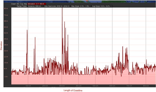
West Coast of Peninsular Malaysia has its coastline along Malacca Strait that runs from Singapore to Thailand as shown in Figure 1. An investigation of the elevation profile of the coastal zones using google earth (Figure 2) revealed that the area comprises of low-elevation areas like most coastal regions. More than 80% of the coastal zone profile has elevation below 10 m. The low-lying coastal regions are highly populated, urbanized, and developed with dense infrastructure distribution (Hamid et al. 2018; Muslim et al. 2020), which makes them vulnerable to the harmful impacts of sea level rise. Its area encompasses Kuala Lumpur, the capital of Malaysia, and the new administrative centre, Putrajaya. States along the coastline include Perlis, Kedah and Penang to the North, Johor and Melaka to the South, Perak and Selangor to the Central.

Figure 1. Map of the Malaysia Sea showing Malacca strait and the locations of West Peninsular tide gauges. Source: Author.

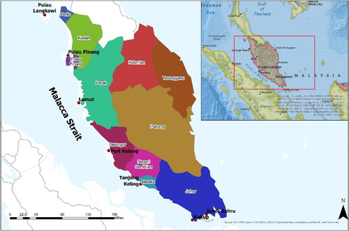
Figure 2. Elevation profile of West Peninsular Coastline.

Marine Data including Sea Level Anomaly (SLA), Sea Surface Temperature (SST), Sea Surface Salinity (SSS), and Sea Surface Density (SSD) were obtained from Copernicus Marine Environment Monitoring Service (CMEMS). SLA is the altimeter satellite gridded sea level anomalies computed with respect to a twenty-year 2012 mean. The SLA is estimated by optimal interpolation, merging the measurement of many altimeter missions such as Jason-3, Sentinel 3, ERS1/2, TOPEX/Poisedon, Jason-1/2 and Envisat. All relevant geophysical corrections, including ionospheric delay correction, tropospheric dry and wet component corrections, solid earth tide and oceanic tide corrections, oceanic load tide correction, polar tide correction, electromagnetic error correction, instrument correction, and inverted barometer correction have been applied. Sea Surface Temperature (SST) is the surface temperature of the sea measured in ^oC. Sea Surface Salinity (SSS) is measured in part per thousand while the Sea Surface Density (SSD) is measured in kg/m³. CMES does not provide mean sea level pressure, so this is acquired from Copernicus Climate Data Store. Atmospheric data including rainfall, total cloud cover and wind speed are also downloaded from the Copernicus Climate Data Store. Various studies have reported that these variables have significant impacts on sea level variation (Sithara et al. 2020). For instance, Longshore winds is a key variable influencing sea level variability on the eastern margins of the ocean (Sturges and Douglas 2011), through its role in moving warm water from one part of the sea to another (Muslim et al. 2020). All the data are gridded monthly mean datasets between January 1993 and October 2019. Tide gauge data are acquired from Permanent Service of Mean Sea Level . The 7 tide gauge stations situated in strategic locations around West Peninsular Malaysia coastlines within the Malacca strait sea (Table 2) were used.

Table 2. Tide gauge stations at the West Peninsular Malaysia.

Station ID	Station name	Region	Established	LAT	LON	% completeness	Near GNSS Station
1676	Pulau Langkawi	Penninsular (North West)	1986	6.431	99.764	96	No
1595	Pulau Pinang	Penninsular (North West)	1985	5.422	100.347	93	No
1594	Lumut	Penninsular (North West)	1984	4.240	100.613	93	No
1591	Port Kelang	Penninsular (West Central)	1984	3.050	101.358	90	No
1593	Tanjung Keling	Penninsular (West Central)	1984	2.215	102.153	94	GPS MELAKA (JUML)
1677	Kukup	Penninsular (South West)	1986	1.325	103.443	97	No
248	Johor Bahru	Penninsular (South West)	1984	1.462	103.792	91	No

4. Methodology

4.1. Feature selection

Identifying the relevant features to train the model is key to building an optimal predictive model. Including irrelevant inputs or data with minimal significance will increase the training time and introduce noise. This confuses the model and negatively affects the model accuracy. Correlation analysis is employed to select the best feature to train the models. This involves computing a pairwise correlation of all the variables. Heat map of the correlation of ocean-atmospheric variables with sea level change at Johor Bahru is shown in figure 3 below. From the heat map, it is deduced that the atmospheric pressure at the surface and the mean sea level pressure have equal influence on the SLA with correlation value of 0.15. This similarity pattern is the same across all stations. Hence, mean sea level pressure is excluded from further processing to avoid collinearity issue. This is similar to the approach used by Sithara et al. (2020) to eliminate surface pressure and ocean current variables that are inter-correlated with mean sea level pressure before training SVR model to predict sea level variation at Willington Island tide gauge station.

Figure 3. Heat Map of ocean-atmosphere variable correlation matrix for Johor Bahru.

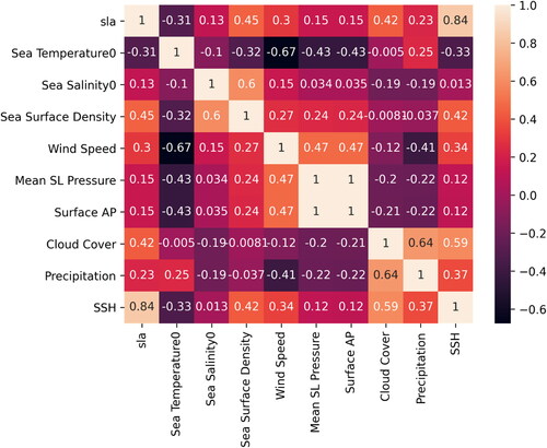
Other features are used as input variables to train the model while SLA is the target. It is noteworthy to mention that Sea Surface Height (SSH) is not included among the variables for the model training. SSH is the relative sea level measured by the tide gauge stations, thus the reason for the strong correlation with SLA. Although SSH could as well be adopted as the target variable in the model training, we opted to use SLA of the altimetry data since it does not contain missing values and has more recent data (till October 2019) than the SSH variation whose record in the PSMSL extends only up to 2018.

Moreover, altimetry satellite derived sea level is referenced to earth’s coordinate system, representing actual sea level variation contrary to sea level data from tide gauges that includes vertical land movement (VLM) since it is referenced to a local datum. The statistical summary of the sea level data and ocean-atmospheric variables is shown in Table 3.

Table 3. Summary Statistics of the ocean-atmosphere variables for 7 stations in West Peninsular Malaysia.

Station name	Statistics	SLA (m)	SST (^oC)	SSS (0.001)	SSD (kg/m^3)	Wind Speed (ms-1)	Surface AP (hPa)	Cloud Cover	Precipitation (m)
Pulua Langkawi	mean	0.0361	29.63	31.95	1019.73	3.15	100786	0.78	0.0060
	std	0.0771	0.79	0.41	0.14	0.77	89.8845	0.13	0.0036
	min	−0.1882	27.57	30.64	1019.31	1.81	100547	0.38	0.0001
	max	0.2458	31.47	32.64	1020.05	5.76	101025	0.96	0.0171
Pulau Pinang	mean	0.0417	29.60	31.32	1021.10	2.22	100779	0.81	0.0069
	std	0.0770	0.64	0.57	0.18	0.34	84.1862	0.11	0.0032
	min	−0.1759	28.43	30.20	1020.43	1.66	100550	0.45	0.0008
	max	0.2548	30.93	32.16	1021.50	3.98	101020	0.96	0.0186
Lumut	mean	0.0451	29.72	31.71	1019.55	2.64	100945	0.83	0.0074
	std	0.0800	0.50	0.49	0.14	0.45	84.2292	0.09	0.0030
	min	−0.2035	28.20	29.78	1019.01	1.70	100715	0.49	0.0016
	max	0.2657	31.06	32.49	1020.00	4.37	101185	0.96	0.0187
Port Kelang	mean	0.0406	29.60	31.76	1019.64	2.90	100814	0.82	0.0079
	std	0.0791	0.60	0.47	0.16	0.53	83.1363	0.09	0.0033
	min	−0.1582	27.83	29.40	1019.00	1.88	100579	0.48	0.0009
	max	0.2441	31.06	32.42	1020.08	4.97	101045	0.96	0.0214
Tanjung Keling	mean	0.0369	29.41	31.63	1019.73	2.70	100560	0.82	0.0064
	std	0.0746	0.79	0.52	0.25	0.54	83.4715	0.08	0.0026
	min	−0.1187	27.07	28.63	1019.20	1.76	100315	0.52	0.0002
	max	0.2511	31.26	32.59	1020.28	4.72	100783	0.97	0.0241
Kukup	mean	0.0300	29.18	30.75	1019.81	3.62	100916	0.80	0.0065
	std	0.0736	0.82	0.63	0.33	0.72	83.2241	0.09	0.0026
	min	−0.1399	27.75	29.38	1019.32	2.23	100668	0.48	0.0001
	max	0.2440	30.47	31.57	1020.51	5.51	101134	0.95	0.0165
Johor Bahru	mean	0.0327	29.16	30.73	1019.81	2.39	100632	0.81	0.0073
	std	0.0870	0.76	0.62	0.33	0.54	83.1663	0.08	0.0028
	min	−0.1520	27.61	29.28	1019.32	1.45	100384	0.51	0.0006
	max	0.2862	31.04	31.55	1020.51	3.95	100852	0.96	0.0157

4.2. Data transformation

Since the dataset comprise of many features with varying range and units, and the models are highly sensitive to feature scale, it is very important to scale the feature values to a standard scale. Data standardization was applied to transform the values to a mean of 0 and standard deviation of 1. This method transforms feature X to X’ using equation 3(3) $$X^{\mathrm{\prime }}=\mathrm{ }\frac{X-\mu }{\sigma }$$(3) below: (3) $$X^{\mathrm{\prime }}=\mathrm{ }\frac{X-\mu }{\sigma }$$(3) where µ and $\sigma$ are the mean and standard deviation of the feature values respectively.

4.3 ARIMA, SVR AND LSTM

Autoregressive integrated moving average, ARIMA(p,d,q), is a popular and commonly used classical time series model (Moslem Imani et al., 2014a, 2014b). p is the order of autoregression, d is the order of difference required to achieve stationarity in the time series and q is the order moving average (Box et al. 2015; Imani, You, & Kuo, 2014a, 2014b). ARIMA, like many other classical time series models such as exponential smoothing and least squares, is a linear time series model where y(t) is related to its previous (lag) data based on linear function (Moslem Imani et al., 2014a, 2014b). Depending on the nature of the data series, different variation of the model is possible; AR(p) is a special case of ARIMA where d and q are zero while MA(q) is a case where p and d are zero. There is also seasonal ARIMA, ARIMA(p,d,q)(P,D,Q)s where the P,D,Q are the AR, integrated difference and Moving Average order of the seasonal term. The model identification of ARIMA is based on the behavior of partial auto-correlation and auto-correlation functions (PACF and ACF) (Box et al. 2015).

SVR, a regression variant of the popular support vector machine, is a model that uses high dimensional feature spaces but penalizes the resulting complexity using a penalty term that is augmented with the error function and is suitable for fitting high dimensional data with comparatively lesser samples (Krell 2018).

LSTM has complex architecture that gives the network capability to keep layer information from past inputs for long storage to be used in subsequent training which make it suitable for time series application where current values depend on past records (Ishida et al. 2020).

4.4. Model development

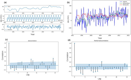
The standard 70:30 ratio for training and testing datasets was adopted (Lai et al. 2020). Monthly Sea Level Altimetry (SLA) data were employed in training and testing the model, and four predictive scenarios were explored. In the first scenario, univariate predictive model was developed using sea level data for ARIMA model. For this development, no driving process was included for the training. To build the ARIMA model for this scenario, the sea level dataset was examined for stationarity by decomposing the sea level data followed by calculation of rolling statistics and performance of dickey-fuller test. The decomposed time series and rolling statistics graph of Johor Bahru sea level data are shown in Figures 4a and 4b, respectively. Visual inspection of these figures indicates oscillation and a rising trend in the series, so we differenced the timeseries to achieve stationarity. The ACF and PACF functions were plotted (Figures 4c and 4d) to identify other model parameters (P,Q, p and q). This was followed by the grid search method to find the hyperparameters for optimal model. Finally, several models were identified, and the Akaike information criterion (AIC) and Bayesian Information Criterion (BIC) (Box et al. 2015) were adopted for model selection.

Figure 4. Time series analysis plots for Johor Bahru showing (a) sea level decomposed into trends, seasonality and residuals. (b) rolling mean statistics (c) autocorrelation (d) Partial autocorrelation.

Ocean variables were used to build the predictive models for the second scenario while Atmospheric variables were used to build the predictive model of the third scenario. The inputs for the models for the second scenario include sea surface temperature, sea surface salinity and sea surface density. wind speed, total cloud cover, surface atmospheric pressure and precipitation Were used as inputs for the third scenario. We used both ocean and atmospheric variables for the predictive model in the fourth scenario. SVR and LSTM were trained based on each of these scenarios and the hyper parameters of the SVR model were determined after a grid search time series cross validation method. Optimal parameters used include radial basis function (rbf), cost value of 10 and epsilon of 0.001. The LSTM model configuration involves three hidden layers, batch size of 32, Adam optimizer and one output layer, with each hidden layer having a dropout rate of 20% and 50 memory units.

4.5. Assessment of prediction accuracy

Assessing the prediction accuracy of the models is vital for validating their performance and this can be done using many metrics (Hyndman and Koehler 2006). In this study, correlation coefficient, R, is used to assess the prediction accuracy of the three models. These assessment metrics are commonly used in many prediction studies (Barbosa et al. 2004; Y. Fu et al. 2019; Yanguang Fu et al. 2019). R is a goodness of fit assessment that measure the efficiency of the model to replicate the observed values based on the extent of total deviation of model outcomes.

4.6. Trend estimation

The trend was estimated using robust fit regression techniques since robust fit analysis optimizes solution determination and outlier’s detection (Din et al. 2017). This approach was used to fit a linear trend to sea surface height time series of each station with an iteratively re-weighted least squares (IRLS) technique wherein weights of observations are adjusted according to the deviations from the trendline to re-fit the trendline repeatedly until the solution converges (Holland and Welsch 1977).

5. Result and discussion

5.1. Correlation pattern

The pattern of correlation of ocean and atmospheric variables with sea level varies across the stations considered in this study. Figure 5 below shows the heatmap of the correlation of processes with sea level for Johor Bahru (5a) and Lumut (5 b). For Lumut, cloud cover has the highest correlation with sea level variation while sea temperature has the least. The pattern in Johor Bahru is however different with sea surface density having the highest correlation and sea salinity the least.

Figure 5. Heat map of ocean-atmosphere correlation for Johor Bahru (a) and Lumut (b).

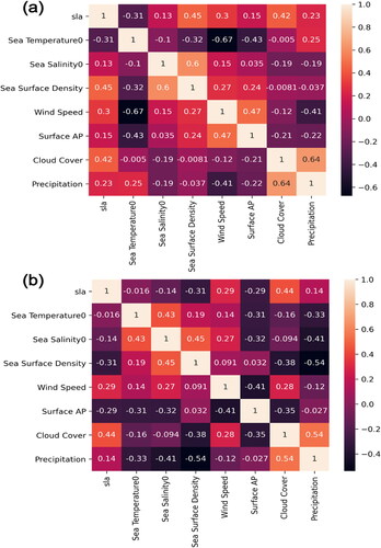
The correlation of ocean-atmospheric variables with sea level variation for all stations are presented in Table 4 below. Wind speed, precipitation and cloud cover have consistent, strong, positive correlation across all stations while correlation pattern of other variables change across the stations. Cloud cover has the most dominating influence at all stations followed by wind speed and precipitation.

Table 4. Correlation of ocean-atmospheric variables with sea level.

	Sea Temperature	Sea Salinity	Sea Surface Density	Wind Speed	Surface AP	Cloud Cover	Precipitation
Pulua Langkawi	0.043	−0.01	−0.026	0.0085	−0.027	0.47	0.28
Pulau Pinang	0.11	−0.053	−0.35	0.19	−0.25	0.45	0.25
Lumut	−0.016	−0.14	−0.31	0.29	−0.29	0.44	0.14
Port Kelang	0.083	−0.31	−0.41	0.21	−0.25	0.42	0.28
Tanjung Keling	−0.0083	−0.3	−0.17	0.2	−0.083	0.41	0.079
Kukup	−0.24	−0.063	0.24	0.14	0.049	0.44	0.0042
Johor Bahru	−0.31	0.13	0.45	0.3	0.15	0.42	0.23

5.2. Influence of oceanic and atmospheric processes on sea level prediction

Comparison of models trained on Ocean Variables (OV) with models trained on Atmospheric Variables (AV) show that atmospheric processes have more influence on model prediction than ocean processes. The R accuracy of the models for the four scenarios is presented in Table 4. For SVR, higher R accuracy is obtained with atmospheric variables for all the stations except at Port Kelang where ocean variables produced the better R accuracy. Excluding Port Kelang, the performance of SVR model prediction is improved by around 7% to 29% when atmospheric variables are used for model training, relative to the accuracy of same model trained with ocean variables. The mean of R accuracy of the SVR predictive models trained with atmospheric variables is 0.720 and mean R accuracy of 0.597 was obtained when the same model is trained with ocean variables. Similarly, for LSTM, better R accuracy is obtained with atmospheric variables at all the stations (Table 5). Relative to the accuracy of the LSTM models trained with ocean parameters, the prediction performance of LSTM model improved by 0.5–31% when trained with atmospheric parameters. The mean of R accuracy of LSTM model trained with atmospheric and ocean variables is 0.810 and 0.643, respectively. Training with combined Ocean-Atmospheric variables (OAV) improved the models’ prediction at all 7 stations but by only a small percentage for both SVR and LSTM. This suggests that sea level variation in West Peninsular Malaysia is majorly dominated by ocean and atmospheric processes with the latter having greater influence.

Table 5. R accuracy of ARIMA, SVR and LSTM models for different scenarios at all station.

	ARIMA	SVR					LSTM
Station	No input	OV	AV	OAV	% Increase of AV relative to OV	% Increase of OAV relative to AV	OV	AV	OAV	%Increase of AV relative to OV	% Increase of OAV relative to AV
Langkawi	0.882	0.591	0.749	0.769	21.095	2.601	0.637	0.839	0.879	24.076	4.768
Pinang	0.605	0.549	0.726	0.742	24.380	2.156	0.595	0.816	0.852	27.083	4.412
Lumut	0.683	0.626	0.679	0.718	7.806	5.432	0.672	0.769	0.828	12.614	7.672
Port Kelang	0.835	0.699	0.659	0.712	−6.070	7.444	0.745	0.749	0.822	0.534	9.746
Tanjung Keling	0.703	0.619	0.706	0.737	12.323	4.206	0.665	0.796	0.847	16.457	6.407
Kukup	0.573	0.521	0.743	0.769	29.879	3.381	0.567	0.833	0.839	31.933	0.720
Johor Bahru	0.692	0.575	0.776	0.792	25.902	2.020	0.621	0.866	0.902	28.291	4.157
Mean of R	0.710	0.597	0.720	0.748	16.474	3.891	0.643	0.810	0.853	20.141	5.412

*OV, Ocean variables; AV, Atmospheric Variables; OAV, Ocean Atmospheric variables.

Earlier studies have also discovered this pattern of strong atmospheric influence on sea level variation around the Indian ocean. Analysis of ANN model performance by Zubier and Eyouni (2020) revealed that atmospheric variables play the major role in sea level variation over east central red sea. It has also been discovered in a recent study of sea level prediction in the Sabah state of Malaysia by Muslim et al. (2020) that atmospheric variables have profound impact on sea level prediction over the study area. The findings from these studies agree with this current study except that influence of ocean variables are not considered in those studies. On the contrary, Sithara et al. (2020) reported that ocean variables such as sea surface temperature, sea surface salinity and mean sea level pressure have dominant impact on sea level prediction models over Willington Island. All these findings confirm that processes driving sea level vary across coasts and regions. Identifying the dominant local variables is therefore vital in building optimal sea level prediction model.

5.3. Assessment of models’ performance

The comparison of the models’ performance in predicting sea level variations for all stations in the study area (Table 5) show that LSTM generally outperforms SVR and ARIMA. The superior performance of LSTM model is due to its complex architecture that gives the network capability to keep layer information from past inputs for long storage to be used in subsequent training (Ahmed et al. 2010; Makridakis et al. 2018). This makes the model suitable for time series application where current values depend on past records. The mean of R accuracy of optimal performing LSTM, SVR and ARIMA models at all stations are 0.853, 0.748 and 0.710, respectively (Table 5). From the analysis of these results, it can be inferred that the performance of prediction models is largely influenced by the dominant processes at the location of interest. For example, LSTM model trained with ocean-atmospheric parameters outperforms SVR and ARIMA in all scenarios and at all stations except Langkawi station where ARIMA model has the best performance with R accuracy of 0.882. This is possibly due to the minimal influence of ocean-atmospheric processes at this station. The combined correlation of the ocean and atmospheric processes is lowest at this region thereby implying that sea level variation is tide dominated at the region. Consequently, ARIMA model, being able to learn the pattern of sea level variation based on univariate time series modelling has the best performance.

Comparing the performance of the optimal models in this study with performance of models in other similar studies trained with fewer input variables show an improvement in prediction performance. The R-accuracy of the optimal models on test dataset across seven stations considered in this study ranges from 0.822 to 0.902. Muslim et al. (2020) trained MLP-ANN and ANFIS with two scenarios of different combinations of wind direction, wind speed, cloud cover and precipitation. The optimal models at the three stations have R accuracy of 0.7963, 0.7223 and 0.8274 for Kudat stations, Sandakan and Kota Kinabalu respectively. Lai et al. (2019) developed sea level predictions for three stations in Malaysia by training SVR and GP models with precipitation, cloud cover and sea surface temperature variables. The R-accuracy of the optimal models on test dataset ranges between 0.728 and 0.863. This study revealed that prediction accuracy can be improved by incorporating more ocean-atmospheric variables in model training.

5.4. Trend and pattern of sea level changes

The trend in relative sea level change estimated using robust fit regression technique is presented in Table 6 below. A rising trend in sea level change was observed at all tide gauge stations and the rate ranges from 3.07 $\pm$ 2.07 mm/yr at Tanjung Keling to 5.90 $\pm$ 1.86 mm/yr at Kukup. The average sea level trend of the seven stations is 4.58 $\pm$ 2.46 mm/yr, which is higher than global rate of SLR of 3.2 ± 0.4 mm/yr and 3.1 ± 0.6 mm/yr estimated by Jevrejeva et al. (2014) from satellite altimetry and tide gauges respectively, thus forewarning that there is need to intensify efforts in preparing and protecting the coastal zones from potential impacts of this above normal sea level rise. Patterns of sea level change are distinguished by region. Three stations at the North (Figure 6) and two stations at the central (Figure 7) have similar patterns. Minimum record of sea level at these stations occurred around late 1997 or early 1998 (Dec 1997 for Pulua Langkawi, Pulua Pinang, Port Kelang and Jan 1998 for Lumut) with subsequent return to normal in mid-1998 and significant rise from 1999. Many authors attribute these drastic drops in sea levels to EL Nino event of 1997. In their study, Hamid et al. (2018) acknowledged the impact of El Nino on sea level pattern in the Asian region. Also, Yanguang Fu et al. (2019) discovered that the sea level trend over china sea reduced drastically during the El nino period of 1997 in comparison to other periods. Similar effect was discovered by A. H. Kamaruddin et al. (2017) for East Coast of Peninsular Malaysia. The impact of La Nina event of 2010 on sea level pattern is also observed as maximum values are recorded within this period. In contrast, there is no distinct pattern in sea level change of the 2 South West stations located at the meeting of water of Malacca strait and south china sea (Figure 8) perhaps due to the complexities created by the interaction of the two waters at this region.

Figure 6. Relative SLA pattern for North West Peninsular.

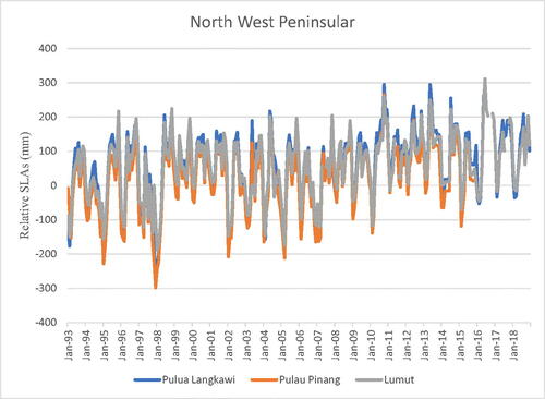
Figure 7. Relative SLA pattern for West Central Peninsular.

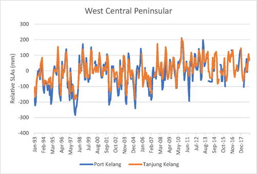
Figure 8. Relative SLA pattern for South West Peninsular.

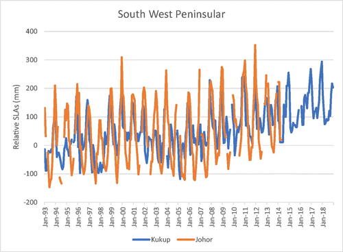
Table 6. Relative Sea Level Trend of the seven tide gauge stations at West Peninsular.

Location	Rate by Robust Fit (mm/yr)	Min			Max		Mean
		Date	Value		Date	Value
Pulau Langkawi	4.14 $\pm$2.20	12/1997		−272	10/2010	295	56.5
Pulau Pinang	4.04 $\pm$2.40	12/1997		−299	10/2010	265	20.4
Lumut	3.31$\pm$ 1.88	01/1998		−189	06/2016	311	54.87
Port Kelang	3.80$\pm$ 2.46	12/1997		−284	10/2010	210	−17.5
Tanjung Keling	3.07 $\pm$2.07	03/2005		−184	10/2010	207	1.0
Kukup	5.90 $\pm$ 1.86	03/2005		−118	12/2017	294	55.9
Johor Bahru	3.88 $\pm$2.67	06/1993		−147	12/2011	352	41.4

6. Conclusion

The goal of this study is to integrate ocean and atmospheric processes in the development of prediction models for local sea-level pattern at 7 tide gauge stations in West Peninsular Malaysia. The objectives include to identify ocean and atmospheric processes driving sea level variation, investigate the influence of these processes on the accuracy of sea level prediction, assess the performance of classical time series, machine learning and deep learning models and estimate the sea level trend over the study area. Ocean variables considered include sea surface temperature, sea surface salinity and sea density while the atmospheric variables considered include surface atmospheric pressure, wind speed, total cloud cover and precipitation. Prediction based on four scenarios with different input combinations were explored. The first scenario employs only sea level data in univariate modelling with ARIMA. SVR and LSTM neural network models were trained on the second, third and fourth scenarios which used ocean variables, atmospheric variables, and combined ocean-atmospheric variables, respectively. Prediction performance of the univariate ARIMA model, each SVR model trained on OV, AV, OAV and LSTM neural network models trained on OV, AV, OAV were compared. Trend in the sea level changes was determined using robust regression techniques based on Iteratively Re-weighted Least Square Method.

This study revealed that cloud cover, wind speed and precipitation have consistent strong positive correlation with sea level variation across all the stations while other variables have varying correlation. Sea level variation in West Peninsular Malaysia is majorly dominated by ocean and atmospheric processes with the latter having greater influence. Combining ocean and atmospheric variables improve the model prediction at all stations but by only a small percentage for both SVR and LSTM models. Comparison of model performance show that LSTM model trained with ocean and atmospheric variables is optimal for predicting sea level variation at all stations except Pulua Langkawi where ARIMA model trained without ocean-atmospheric variables performed best due to the dominating tide influence. This implies that different prediction is suitable for different regions and optimal prediction model depends on the dominating processes at play in each region. Rising trend in sea level change is discovered at all stations with mean value that is higher than global rate, implying that there is need to intensify adaptation efforts to protect coastal zones in the study area.

Disclosure statement

No potential conflict of interest was reported by the author(s).

References

- Ablain M, Legeais JF, Prandi P, Marcos M, Fenoglio-Marc L, Dieng HB, … Cazenave A. 2017. Satellite Altimetry-Based Sea Level at Global and Regional Scales. In A. Cazenave, N. Champollion, F. Paul, & J. Benveniste (Eds.), Integrative study of the mean sea level and its components; p. 9–33. Cham: Springer International Publishing.
- Ahmed NK, Atiya AF, Gayar NE, El-Shishiny H. 2010. An empirical comparison of machine learning models for time series forecasting. Econometric Reviews. 29(5-6):594–621.
- Barbosa SM, Fernandes MJ, Silva ME. 2004. Nonlinear sea level trends from European tide gauge records. Ann Geophys. 22(5):1465–1472.
- Box GE, Jenkins GM, Reinsel GC, Ljung GM. 2015. Time series analysis: forecasting and control. John Wiley & Sons. Hoboken, New Jersey, (USA).
- Cazenave A, Llovel W. 2010. Contemporary sea level rise. Ann Rev Mar Sci. 2(1):145–173.
- Cazenave A, Palanisamy H, Ablain M. 2018. Contemporary sea level changes from satellite altimetry: What have we learned? What are the new challenges? Adv Space Res. 62(7):1639–1653.
- Church JA, White NJ. 2011. Sea-level rise from the late 19th to the early 21st century. Surv Geophys. 32(4-5):585–602.
- Cipollini P, Calafat FM, Jevrejeva S, Melet A, Prandi P. 2017. Monitoring sea level in the coastal zone with satellite altimetry and tide gauges. Surv Geophys. 38(1):33–57.
- Din AHM, Hamid AIA, Yazid NM, Tugi A, Khalid NF, Omar KM, Ahmad AJJT. 2017. Malaysian sea water level pattern derived from 19 years tidal data. Journal Teknologi. 79(5):137-145
- Din AHM, Zulkifli NA, Hamden MH, Aris WAW. 2019. Sea level trend over Malaysian seas from multi-mission satellite altimetry and vertical land motion corrected tidal data. Adv Space Res. 63(11):3452–3472.
- Ehsan MRM, Din AHM, Hamid AA, Adzmi NHM. 2019. Interpretation of sea level variability over Malaysian seas using multi-mission satellite altimetry data. ASM Sci J. 12(Special Issue 2):90–99.
- Eun-Joo L, Jeong-Yeob C, Jae-Hun P. 2020. Reconstruction of sea level data around the Korean Coast using artificial neural network methods. J Coastal Res. 95(sp1):1172–1176.
- Foo WY, Teh HM, Babatunde A-L. 2020. Morphodynamics of the TELUK NIPAH shorelines. Platform: J Eng. 4(1): 29–40
- Fu Y, Zhou X, Sun W, Tang Q. 2019. Hybrid model combining empirical mode decomposition, singular spectrum analysis, and least squares for satellite-derived sea-level anomaly prediction. Int J Remote Sens. 40(20):7817–7829.
- Fu Y, Zhou X, Zhou D, Li J, Zhang W. 2019. Estimation of sea level variability in the South China Sea from satellite altimetry and tide gauge data. Adv Space Res.DOI: https://doi.org/10.1016/j.asr.2019.07.001
- Ghazali NHM, Awang NA, Mahmud M, Mokhtar A. 2018. Impact of sea level rise and tsunami on coastal areas of North-West Peninsular Malaysia. Irrig and Drain. 67:119–129.
- Global Change Research Program. 2019. Climate science special report. https://science2017.globalchange.gov/.
- Hamid AIA, Din AHM, Hwang C, Khalid NF, Tugi A, Omar KM. 2018. Contemporary sea level rise rates around Malaysia: altimeter data optimization for assessing coastal impact. J Asian Earth Sci. 166:247–259.
- Hao Z, Deng M, Zhu Q, Tao B, Chen J, Pan D. 2019. Sea level prediction based on the long time series satellite observations (Vol. 11155). SPIE. Bellingham, Washington, (USA).
- Holgate SJ, Matthews A, Woodworth PL, Rickards LJ, Tamisiea ME, Bradshaw E, … Pugh J. J J o C R. 2012. New data systems and products at the permanent service for mean sea level. Journal of Coast Rese. 29(3):493–504.
- Holland PW, Welsch RE. 1977. Robust regression using iteratively reweighted least-squares. Commun Stat - Theory Methods. 6(9):813–827.
- Horton BP, Kopp RE, Garner AJ, Hay CC, Khan NS, Roy K. 2018. Mapping sea-level change in time, space, and probability. Annu Rev Environ Resour. 43:481–521.
- Hyndman RJ, Koehler AB. 2006. Another look at measures of forecast accuracy. Int J Forecast. 22(4):679–688.
- Imani M, You R-J, Kuo C-Y. 2014a. Analysis and prediction of Caspian Sea level pattern anomalies observed by satellite altimetry using autoregressive integrated moving average models. Arab J Geosci. 7(8):3339–3348.
- Imani M, You RJ, Kuo CY. 2014b. Caspian Sea level prediction using satellite altimetry by artificial neural networks. Int J Environ Sci Technol. 11(4):1035–1042.
- IPCC 2013. Sea Level Change. In: Climate Change 2013: The physical science basis. Contribution of Working Group I to the fifth assessment report of the intergovernmental panel on climate change [Church, J.A., P.U. Clark, A. Cazenave, J.M. Gregory, S. Jevrejeva, A. Levermann, M.A. Merrifield, G.A. Milne, R.S. Nerem, P.D. Nunn, A.J. Payne, W.T. Pfeffer, D. Stammer and A.S. Unnikrishnan]. Retrieved from https://www.ipcc.ch/site/assets/uploads/2018/02/WG1AR5_Chapter13_FINAL.pdf
- Ishida K, Tsujimoto G, Ercan A, Tu T, Kiyama M, Amagasaki M. 2020. Hourly-scale coastal sea level modeling in a changing climate using long short-term memory neural network. Sci Total Environ. 720:137613.
- Jevrejeva S, Jackson LP, Riva REM, Grinsted A, Moore JC. 2016. Coastal sea level rise with warming above 2 °C. Proc Natl Acad Sci USA. 113(47):13342–13347.
- Jevrejeva S, Moore JC, Grinsted A, Matthews AP, Spada G. 2014. Trends and acceleration in global and regional sea levels since 1807. Global Planet Change. 113:11–22.
- Kamaruddin AH, Din AHM, Pa'Suya MF, Omar KM. 2017. Long-term sea level trend from tidal data in Malaysia. Paper Presented at the 2016 7th IEEE Control and System Graduate Research Colloquium, ICSGRC 2016 - Proceeding.
- Kamaruddin AH, Din AHM, Pa'suya MF, Omar KM. (2016). Long-term sea level trend from tidal data in Malaysia. Paper presented at the 2016 7th IEEE Control and System Graduate Research Colloquium (ICSGRC).
- Khairuddin MA, Din AHM, Omar AH. 2019. Sea level impact due to el nino and la nina phenomena from multi-mission satellite altimetry data over Malaysian seas. In Lecture notes in civil engineering. 9:771–792.
- Krell MMJAPA. 2018. Generalizing, decoding, and optimizing support vector machine classification. ArXiv preprint arXiv:1801.04929.
- Lai V, Ahmed NA, Malek MA, Abdulmohsin Afan H, Ibrahim KR, El-Shafie A, El-Shafie A. 2019. Modeling the nonlinearity of sea level oscillations in the Malaysian coastal areas using machine learning algorithms. Sustainability. 11(17):4643.
- Lai V, Malek M, Abdullah S, Latif S, Ahmed A. 2020. Time-series prediction of sea level change in the East Coast of Peninsular Malaysia from the supervised learning approach. IJDNE. 15(3):409–415.
- Makridakis S, Spiliotis E, Assimakopoulos V. 2018. Statistical and machine learning forecasting methods: concerns and ways forward. PLoS One. 13(3):e0194889
- Muslim TO, Ahmed AN, Malek MA, Abdulmohsin Afan H, Khaleel Ibrahim R, El-Shafie A, Sapitang M, Sherif M, Sefelnasr A, El-Shafie A. 2020. Investigating the influence of meteorological parameters on the accuracy of sea-level prediction models in Sabah, Malaysia. Sustainability (Switzerland), 12(3):1193.
- Nicholls RJ, Cazenave A. J s. 2010. Sea-level rise and its impact on coastal zones. Science. 328(5985):1517–1520.
- Nidhinarangkoon P, Ritphring S, Udo K. 2020. Impact of sea level rise on tourism carrying capacity in Thailand. JMSE. 8(2):104.
- Ponte RM, Carson M, Cirano M, Domingues CM, Jevrejeva S, Marcos M, … Zhang X. 2019. Towards comprehensive observing and modeling systems for monitoring and predicting regional to coastal sea level. Rev Art.6(437).doi: https://doi.org/10.3389/fmars.2019.00437
- Pycroft J, Abrell J, Ciscar JC. 2016. The global impacts of extreme sea-level rise: a comprehensive economic assessment. Environ Resource Econ. 64(2):225–253.
- Rahmstorf S. 2012. Modeling sea level rise. Nat Educ Knowl. 3(10): 4.
- Ranjbar A, Cherubini C, Saber A. 2020. Investigation of transient sea level rise impacts on water quality of unconfined shallow coastal aquifers. Int J Environ Sci Technol. 17(5):2607–2622.
- Sarkar MSK, Begum RA, Pereira JJ, Jaafar AH, Saari MY. 2014. Impacts of and adaptations to sea level rise in Malaysia. Asian J Water Environ Pollut. 11(2):29–36.
- Schaefer N, Mayer-Pinto M, Griffin KJ, Johnston EL, Glamore W, Dafforn KA. 2020. Predicting the impact of sea-level rise on intertidal rocky shores with remote sensing. J Environ Manage. 261:110203.
- Shi W, Lu C, Werner AD. 2020. Assessment of the impact of sea-level rise on seawater intrusion in sloping confined coastal aquifers. J Hydrol. 586:124872.
- Sithara S, Pramada SK, Thampi SG. 2020. Sea level prediction using climatic variables: a comparative study of SVM and hybrid wavelet SVM approaches. Acta Geophys. 68(6):1779–1790.
- Srivastava PK, Islam T, Singh SK, Petropoulos GP, Gupta M, Dai Q. 2016. Forecasting Arabian Sea level rise using exponential smoothing state space models and ARIMA from TOPEX and Jason satellite radar altimeter data. Met Apps. 23(4):633–639.
- Stammer D, Cazenave A, Ponte RM, Tamisiea ME. 2013. Causes for contemporary regional sea level changes. Ann Rev Mar Sci. 5:21–46.
- Sturges W, Douglas BC. 2011. Wind effects on estimates of sea level rise. J Geophys Res. 116(C6).doi: https://doi.org/10.1029/2010JC006492
- Werner AD, Simmons CTJG. 2009. Impact of sea-level rise on sea water intrusion in coastal aquifers. Ground Water. 47(2):197–204.
- Yi S, Heki K, Qian A. 2017. Acceleration in the Global Mean Sea Level Rise: 2005–2015. Geophys Res Lett. 44(23):11,905–911,913.
- Zhao J, Fan Y, Mu Y. 2019. Sea level prediction in the yellow sea from satellite altimetry with a combined least squares-neural network approach. Mar Geod. 42(4):344–366.
- Zubier KM, Eyouni LS. 2020. Investigating the role of atmospheric variables on sea level variations in the Eastern Central Red Sea using an artificial neural network approach. Oceanologia. 62(3):267–290.