Research on compressive sensing of strong earthquake signals for earthquake early warning

Abstract

Earthquake early warning is an effective method to reduce casualties and losses. Based on the theory of compressive sensing, this paper proposes a strong earthquake signal processing architecture based on compressive sensing for difficulties of the acquisition, transmission and storage of massive strong earthquake data that the large-scale earthquake warning systems faced. Based on this, the observation vector of strong earthquake signal can be obtained with a predetermined compression ratio and used for transmission and storage. When necessary, the observation value is reconstructed to restore the original strong earthquake signal with a high probability. The paper analyzes the selection of sparse basis and observation matrix, discusses the reconstruction algorithms, base pursuit (BP) and orthogonal matching pursuit (OMP), and verifies the feasibility of the whole framework from compressed sampling to data reconstruction through experiments. The proposed framework has brought great convenience to the sampling, transmission, storage, and processing of the earthquake early warning system. It is foreseeable that replacing the traditional Nyquist sampling value with the observation values in the compressive sensing theory will cause a fundamental change in the signal characteristics, which will further affect the theory and technical system of the entire earthquake early warning system.

Keywords:

• Earthquake early warning
• strong earthquake
• compressive sensing
• sparseness
• reconstruction

1. Introduction

Earthquakes are one of the natural disasters that seriously threaten human life and property security. They often cause severe building damage and casualties, result in fires, floods, toxic gas leakage, and the spread of bacteria and radioactive materials, and lead to secondary disasters such as tsunamis, landslides, collapse, and ground fissures. A large amount of energy is released within a short period of time after the earthquake, which can cause devastating damage within tens of seconds or even seconds. The occurrence of earthquakes is beyond human control, which is a common feature of earthquakes and many other natural disasters. The preparation and occurrence of earthquakes are extremely complex, so reliable short-term earthquake predictions are currently not available (Kanamori et al. 1997). But, after the earthquake, if the final scale of the earthquake can be identified by P in the early stage of fault rupture and the earthquake warning information can be sent to the early warning target area by electrical signals before the destructive S wave arrives, areas that receive early warning information can take disaster mitigation measures in advance.

An earthquake of 7.0 magnitudes struck the Hayward fault in the United States in 1868, and then Professor Cooper first proposed the idea of earthquake early warning (Cooper 1868). The greatest significance of earthquake warning is to reduce casualties. Studies have shown that (Xia and Yang 2000): if the early warning time is 3 seconds, the casualties can be reduced by 14%; if it is 10 seconds, the casualties can be reduced by 39%; and if it is 20 seconds, the casualties can be reduced by 63%. Due to the obvious effect on disaster prevention and mitigation (Wang et al. 2009), and since the deployment of the UrEDAS for Shinkansen in Japanese in 1988, the earthquake early warning system has developed rapidly worldwide in the past few decades. At present, more mature earthquake early warning systems have been established in Japan, the United States, Mexico, Turkey, and China, including the systems that serve the people in a certain area or city, and special earthquake early warning systems that serve specific units. After the Wenchuan earthquake in 2008, demand for earthquake warning systems in China has increased sharply, prompting considerable resources to be devoted to the construction of earthquake warning system. The "National Seismic Intensity Rapid Alert and Early Warning Project" intends to encrypt the strong earthquake observation stations in the seismic risk areas. And after its completion, it will bring tens of thousands of observation stations in China, providing a powerful infrastructure for earthquake warning systems.

On the one hand, earthquake monitoring and early warning technology is developing in the direction of multi-dimensional, multi-component, multi-parameter, and high resolution; on the other hand, with the continuous increase in the number and scale of earthquake early warning observation networks, the amount of data collected shows exponential growth and the total seismic data continues to expand (Ma 2008). However, how to effectively transmit and access these massive observation data after acquiring them is an important issue that restricts the further development of earthquake monitoring and early warning systems. Data compression, as an information processing technology, has been well developed and applied, but its development is still relatively weak in the field of earthquake monitoring and early warning. Previous studies have proposed the use of statistical-based coding methods (HUFFMAN coding, arithmetic coding, etc.), dictionary-based coding methods, and transformation-based methods (DCT transform, Fourier transform, etc.) for lossless compression of seismic data, but these methods are rarely seen in practical applications . The Steim2 compression algorithm based on the SEED volume format is commonly used in international and domestic seismic data transmission and local storage. The Steim2 compression algorithm is developed by borrowing the simplest differential compression algorithm in speech compression. It is characterized by lossless compression. And the compression ratio of the algorithm, during the quiet period of the earthquake, is 3.67: 1. However, during the active period of the earthquake, the Steim2 algorithm will have a limited compression capacity and may even fail immediately. Instead, an anomaly phenomenon that the compressed data rate is higher than the uncompressed data rate may occur (Wang et al. 2004; Yang et al. 2019).

With a long-term focus on the transmission and storage of massive data in earthquake early warning systems, we find that the popular compressive sensing theory in recent years is just suitable for the application. Nyquist sampling theorem points out that in order to capture a signal with a specified bandwidth perfectly, analog-to-digital conversion usually needs to be carried out at a sampling rate greater than twice the frequency band. Compressive sensing theory states that if a signal is sparse in a certain orthogonal space, it can be sampled at a frequency much lower than the Nyquist sampling rate, and the signal may be reconstructed with a high probability. Based on the compressive sensing theory, we propose a kind of transmission architecture of signal acquisition for earthquake monitoring and early warning system, which solves the data compression problems, faced by the acquisition and transmission process in earthquake early warning systems and provides new application directions.

2. Compressive sensing

Theoretical research on compressive sensing can be traced back to the 1980s, and recently, it has developed rapidly with the development of compressed sampling and data reconstruction theories. Tao, Candes, Donoho, etc. have relatively completely constructed the theoretical framework of compressive sensing, and mathematically proved that the original signal can be accurately reconstructed using some Fourier transform coefficients (Candes et al. 2006). The core idea is to perform compression and sampling together, achieving compression while sampling. First collect non-adaptive linear observations of the signal, and then use the corresponding reconstruction algorithm to reconstruct the original signal from the observations. At present, CS theory mainly focuses on the construction of the signal's sparse decomposition matrix, the construction of the observation matrix, and the signal reconstruction algorithm (Sarvotham et al. 2005; Baraniuk et al. 2010).

2.1. Basics of compressive sensing

A one-dimensional vector f of length N can be represented by a linear combination of a set of standard orthogonal bases: (1) $$\mathrm{f}=\sum _{\mathrm{i}=1}^{\mathrm{N}}{\mathrm{x}}_{\mathrm{i}}{\mathrm{\psi }}_{\mathrm{i}}\text{\hspace{0.5em}Or\hspace{0.5em}}\mathrm{f}=\mathrm{\Psi }\mathrm{x}$$(1) $\Psi =\left[{\psi }_1\right|{\psi }_2|\dots |{\psi }_N],$ ${\psi }_i$ are column vectors. When the signal f has only K$\ll N$ non-zero coefficients $x_i$ (or coefficients much larger than zero) on the orthogonal basis $\psi ,$ $\psi$ is called the sparse basis of the signal f. The signal f is K-sparse on the orthogonal basis $\psi ,$ and formula (1) is the sparse representation of the signal f.

Looking at the process of compressive sensing, if a measurement matrix $\Phi \in R^{M\times N}(M\ll N)$ and a signal x are known, the linear observation value $y\in R^{M\times 1}$ of the signal under the measurement matrix $\Phi$ can be obtained. (2) $$\mathrm{y}=\mathrm{\Phi }\mathrm{x}$$(2)

Since the dimension M of the observation value y is much smaller than the dimension N of the signal x, the purpose of compression is achieved. Obviously, on the premise of knowing y and $\Phi ,$ we need to consider how to reconstruct the sequence x. Since the dimension of y is much lower than that of x, the solution of formula (2) is not unique. But if the original signal x is K sparsity and y as well as $\Phi$ meets certain conditions, theory proves that the signal x can be accurately reconstructed from the observation value y by solving optimal ${\mathrm{L}}_0$-norm. (3) $$\widehat{\mathrm{x}}=\mathrm{argmin}\left|\right|\mathrm{x}|{|}_0\mathrm{ }\mathrm{s}.\mathrm{t}.\text{ Φx}=\mathrm{y}\mathrm{ }$$(3)

In the formula, $\left|\right|·|{|}_0\mathrm{ }$ is vector ${\mathrm{L}}_0$-norm, which indicates the number of non-zero elements in the vector x. The signal sparse decomposition described by formula (3) is a minimization problem based on the 0-norm, a NP problem, and it is very difficult to directly solve it. Donoho, Tao et al. have proved that when the coefficients required are sufficiently sparse, the solution of 0-norm optimal problem and 1-norm optimal problem are equivalent (Donoho 2006; Candes and Tao 2006). Therefore, when the signal contains no noise, the transformation of 0-norm optimization problem to 1-norm linear programming problem can be described as: (4) $$\widehat{\mathrm{x}}=\mathrm{argmin}\left|\right|\mathrm{x}|{|}_1\mathrm{ }\mathrm{s}.\mathrm{t}.\text{ Φx}=\mathrm{y}\mathrm{ }$$(4)

The development of compressive sensing theory is also a gradual evolution process. At first, the models in the candes and donoho articles were directly aimed at sparse signals, such as formula (2). It was later found that many signals x are not sparse in practical applications, but $a={\Psi }^{\mathrm{\prime }}x$ is obtained by some orthogonal transformations ${\Psi }^{\mathrm{\prime }},$ where a is sparse and ${\Psi }^{\mathrm{\prime }}$ is the transpose of $\Psi ;$ although x is not sparse here, it can be transformed into sparse a by transforming ${\Psi }^{\mathrm{\prime }},$ which then conforms to the compressive sensing model, that is: (5) $$\mathrm{y}=\mathrm{\Phi }\text{a\hspace{0.5em}Or\hspace{0.5em}}\mathrm{y}=\mathrm{\Phi }{\mathrm{\Psi }}^{\mathrm{\prime }}\mathrm{x}$$(5)

Therefore, the research on sparse transformation is the focus of this problem.

2.2. Sparsity and observation matrix

The premise of CS theory is that the signal is sparse or compressible, however, in practice, the strong earthquake signals obtained by direct analog-to-digital conversion are usually not standard sparse signals, and one method is to obtain sparse signals in the transform domain through specific transformations. Reasonably select the sparse basis Ψ so that the number of sparse coefficients of the signal is as small as possible, which is not only conducive to improving the speed of collecting signals, but also reducing the resources occupied by the storage and transmission of signals.

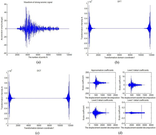
The representation of strong earthquake signals in the time domain is usually a discrete data set recorded by the strong earthquake recorder when earthquake occurs, in this sense, the representation of strong earthquake signals in the time domain is not sparse. Fortunately, the representation of strong earthquake signals in other transform domains can be analyzed. First, the effective part of the strong earthquake signal is mostly concentrated in the low frequency band, so the appropriate selection of the spectrum length can achieve the effects that representations in low frequency band are not zero but most of them in high frequency band are zero. Therefore, the strong earthquake signal is sparse in the frequency domain and can be represented by a discrete Fourier transform. In addition, the paper will discuss the sparsity of discrete cosine transform (DCT) and wavelet transform, as shown in Figure 1. The subsequent experiments in section 4.1 will fully show the applicability of the three sparse bases to strong earthquake signals.

Figure 1. Strong earthquake signal and sparse bases, (a) is a waveform of strong earthquake signal, (b) is the discrete Fourier transform of (a), (c) is the discrete cosine transform of (a), (d) is the decomposition of wavelet (db8) of (a).

In compressive sensing, a stable observation matrix needs to be selected. According to CS theory, in order to ensure that the linear observation can maintain the original structure of the signal, the observation matrix must satisfy the restricted isometry property(RIP) condition (Li et al. 2013; Jiao et al. 2011; Dang et al. 2015): (6) $$(1-{\mathrm{\delta }}_{\mathrm{k}}){\Vert \mathrm{\alpha }\Vert }_2^2\le {\Vert \text{ΦΨα}\Vert }_2^2\le (1+{\mathrm{\delta }}_{\mathrm{k}}){\Vert \mathrm{\alpha }\Vert }_2^2$$(6) $$\mathrm{i}.\mathrm{e}.\mathrm{ }\mathrm{ }(1-{\mathrm{\delta }}_{\mathrm{k}}){\Vert \mathrm{\alpha }\Vert }_2^2\le {\Vert \mathrm{y}\Vert }_2^2\le (1+{\mathrm{\delta }}_{\mathrm{k}}){\Vert \mathrm{\alpha }\Vert }_2^2,\mathrm{ }{\mathrm{\delta }}_{\mathrm{k}}\in \left(0,1\right)$$

Common observation matrices that satisfy the restricted isometry property are: Gaussian random matrix, Bernoulli random matrix, sparse random measurement matrix, partial Fourier matrix, partial Hadamard matrix, etc(Wang et al. 2014a; Wang et al. 2014b; Candes et al. 2006; Zhang et al. 2010; Fang et al. 2008; Haupt et al. 2010; Bajwa et al. 2007).

In the experiments in section 4.2 of the paper, Gaussian random matrices, Bernoulli random matrices, and sparse random measurement matrices have all achieved good experimental results.

2.3. Signal reconstruction

The high-resolution original signal x can be recovered from the observed value y in formula (2) according to compressive sensing theory, that is, signal reconstruction. The reconstruction algorithm is of great significance for the accurate reconstruction of the compressed signal and the accuracy verification during the sampling process. In 1999, Donoho et al. has proposed the basis pursuit (BP) algorithm (Chen et al. 2001), the BP algorithm uses the 1-norm of the representation coefficient to measure its sparseness, and describe the sparse representation signal problem as a type of constrained optimization problem, i.e., formula (4) by minimizing the 1-norm of the representation coefficient. And finally solve the problem by solving the linear programming problem (Do et al. 2008; Efron et al. 2004; Rosasco et al. 2009).

The greedy algorithm is another commonly used method, whose core idea is to select a local optimal solution for each iteration, hoping to select the best atom representing the signal, so as to continuously approach the original signal. Mallat and Zhang first proposed a matching pursuit (MP) algorithm based on greedy ideas in 1993 (Tropp and Gilbert 2007). Subsequently, based on the MP algorithm, several improved algorithms have been proposed, such as the orthogonal matching pursuit (OMP) (Pati et al. 1993; Mallat and Zhang 1993).

The process involved the orthogonal matching pursuit algorithm (OMP) is that calculate the inner product of the information margin and the column vector in the measurement matrix, then select the index of the column with the greatest correlation into the supporting index set, and calculate the residual, the calculation expression is $r\_n=y-\mathit{Aug}\_t\times \mathit{Aug}\_y,$ which is the basis of the next iteration. $\mathit{Aug}\_t$ is the atomic support set determined in the current iteration, and $\mathit{Aug}\_y$ estimation of the signal based on the atomic support set in this iteration. This process is repeated until K atoms (equivalent to sparsity) are selected. There is anorthogonalization process after atoms are selected into the support set at each stage, that is, Gram-Schmidt orthogonalization of the atoms. And then project the measurement signal to the orthogonal zed atomic support set, calculate the residual to ensure that the residual of this iteration are orthogonal to the atoms in the atomic support set. This is exactly the origin of the name, OMP. OMP algorithm precisely introduces the orthogonalization process to ensure the optimality of the iterative solution, thereby greatly reducing the iteration times.

The specific steps of the OMP algorithm are as follows:

Input parameters: measurement matrix $\Phi ,$ recovery matrix $T=\Phi {\Psi }^{\mathrm{\prime }},$ M-dimension measurement signal y, the sparsity K of N-dimension sparse signal x.

Output parameters: K sparse approximation signal hat_x of the N-dimension sparse signal x, reconstruction error.

Initialization: residual r_n = y, incremental matrix (atomic support set) Aug_t=$\mathrm{\varnothing },$ iteration number 1;

Step 1: Calculate the inner product of the residual and each atom (column vector) in the measurement matrix;

Step 2: Find the position corresponding to the maximum projection coefficient (inner product value) and its corresponding atoms, expand the incremental matrix (atomic support set) Aug_t, remove the column of the corresponding position in the recovery matrix;

Step 3: Calculate the orthogonal projection of the measured signal y in the incremental matrix space, and use the least square method to obtain the sparse approximation solution, aug_y=(Aug_t'*Aug_t)^(-1)*Aug_t'*y;

Step 4: Calculate residual r_n = s-Aug_t*aug_y, update iteration times;

Step 5: Stop if the condition of stopping iteration is satisfied, otherwise turn to step 1 and continue. After stopping, output K sparse approximation signal hat_y, obtain time domain signal hat_x by inverse Fourier transform.

As mentioned, the step 1 in OMP is to calculate the inner product of the residual and each atom (column vector) in the measurement matrix. The geometric interpretation of vectors’ inner products is the product of the projection of one vector on another vector, that is, the product in the same direction. From the value of the inner product, the degree of proximity of the two vectors in the direction can be seen.

3. Compressive sensing of strong earthquake signals

For strong earthquake signal, according to the CS theory, an observation matrix Φ which is uncorrelated with sparse base Ψ can be used for the linear projection transformation of strong earthquake signals frame by frame (frame length: N), then obtain the observation vector y. The dimension M of the observed value y is usually much smaller than the dimension N of the signal x. M/N is the ratio of the length of the observed vector to the length of the original strong earthquake signal frame vector, which is defined as the compression ratio. When N is fixed, the larger M is, the larger the compression ratio is; when M is fixed, the larger N is, the smaller the compression ratio is. The compression ratio reflects the degree of compression of the observed value length obtained in CS compressed sampling, compared to that in the traditional Nyquist sampling.

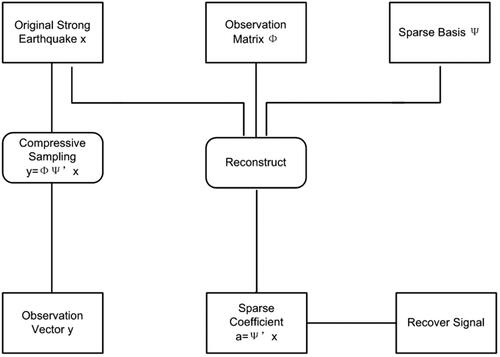
Strong earthquake signals are often a time-varying, non-stationary random process. Therefore, in the compressive sensing of strong vibrations based on CS theory, compressed sampling is performed on each frame of strong earthquake signals based on formula (5) to obtain a linear observed value y, which reduces the cost of storage or communication transmission. After the observed value y is transmitted to the receiver, it can be reconstructed and synthesized the original strong earthquake signal. As shown in the principle block diagram in Figure 2, the key issues that need to be studied include: the construction of sparse bases, the selection of observation matrices, and reconstruction algorithms.

Figure 2. Principle block diagram of compressive sensing of strong earthquake signals.

Based on the principle analysis, this paper gives a practical flow chart of compressive sensing of strong earthquake signals in Figure 3. Different from the principle block diagram, the flow chart considers practical maneuverability. Considering the efficiency problem of compressive sampling and reconstruction algorithm, this paper puts forward the concept of frame. Calculating the strong earthquake signals by framing improves the recovery of signals while taking into account the efficiency of calculation and is more conducive to the subsequent data analysis and processing in the earthquake early warning system, which will be evaluated in section 4.3.

Figure 3. Flow chart of compressive sensing of strong earthquake signals.

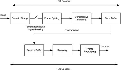
As mentioned earlier, the prerequisite for the application of the compressive sensing method is that the signal must be sparse, and it has been proved that the projection of the strong earthquake signal to the corresponding sparse domain is sparse. However, in the record of the strong earthquake data, there will always be records of pure noise before and after the seismic wave arrives. These noise data do not meet the sparse conditions, so the compressed sampling and reconstruction calculation are infeasible. Therefore, before the process of compressive sensing, a step of picking strong seismic waveforms is added, and compressive sampling and reconstruction calculation are performed only on the effective strong earthquake signals.

4. Performance evaluation experiments

The database in this paper includes Japan's KiK-net records of strong earthquakes, as well as the records of the Wenchuan earthquake and Lushan earthquake. In the evaluation experiment of compressive sensing based on strong earthquake signals, in order to reflect the completeness of data covering range, strong earthquake waveforms with different magnitudes and epicenter distances are selected from the database for compressive sampling and reconstruction experiments. The sampling rate of the selected data records is 100sps or 200sps.

Many factors should be considered in the compressive sampling and reconstruction experiments of strong earthquake signals, such as sparse basis, measurement matrices, reconstruction algorithm and so on, in addition to frame length, compression ratio and so on. These factors will be evaluated in 3 experiments respectively below.

Signal-to-noise ratio (SNR) and mean square error (MSE) are used to measure the quality of reconstructed strong earthquake signals (Wang et al. 2014a). (7) $$\mathrm{SNR}=10\log \left(\frac{\sum _{\mathrm{i}=1}^{\mathrm{N}}{\mathrm{x}}_{\mathrm{i}}^2}{\sum _{\mathrm{i}=1}^{\mathrm{N}}{\left({\mathrm{x}}_{\mathrm{i}}-{\widehat{\mathrm{x}}}_{\mathrm{i}}\right)}^2}\right)=10\log \left(\frac{{\Vert {\mathrm{x}}_{\mathrm{i}}\Vert }_2^2}{{\Vert {\mathrm{x}}_{\mathrm{i}}-{\widehat{\mathrm{x}}}_{\mathrm{i}}\Vert }_2^2}\right)$$(7) (8) $$\mathrm{MSE}=\frac{\sum _{\mathrm{i}=1}^{\mathrm{N}}{\left({\mathrm{x}}_{\mathrm{i}}-{\widehat{\mathrm{x}}}_{\mathrm{i}}\right)}^2}{\mathrm{N}}=\frac{{\Vert {\mathrm{x}}_{\mathrm{i}}-{\widehat{\mathrm{x}}}_{\mathrm{i}}\Vert }_2^2}{\mathrm{N}}$$(8)

N is the frame length, that is, the number of strong seismic data in a frame. In addition, the definitions used later in this paper are:

Measurement M, i.e., the number of compressed samples

Compression ratio M/N;

Average signal-to-noise ratio of the same frame SNR_Aver, that is, the average signal-to-noise ratio obtained from multiple reconstruction experiments of the same frame.

Average signal-to-noise ratio of different frames F_AverSNR, i.e., the average signal-to noise ratio obtained from the reconstruction experiments of the different frames in the whole strong earthquake record.

Average mean square error of different frames F_AverMSE, i.e., the average mean square error obtained from reconstruction experiment of different frames in the whole strong earthquake record.

4.1. Selection of sparse bases

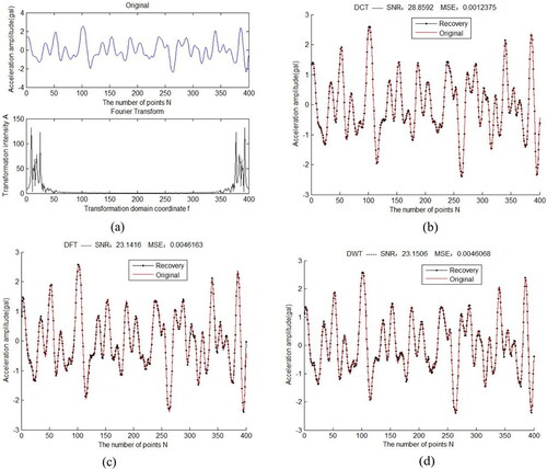
The applicability of discrete Fourier transform basis (DFT), discrete cosine transform basis (DCT), and discrete wavelet transform basis (DWT) to strong earthquake signals is observed in this experiment. Define the frame length N = 400 and select a frame of strong earthquake data, the fixed measurement number M = 240. Use Gaussian random matrix as the measurement matrix, the OMP algorithm as the reconstruction algorithm, and transform three kinds of sparse bases in the experiments.

First, according to formula (5), use three kinds of sparse base to perform compressive sampling and reconstruction experiment on a frame of strong earthquake signal, as shown in Figure 4. It can be seen that for a single experiment, the effect of DCT base is the best, and the effect of DFT base and DWT wavelet base is equivalent.

Figure 4. A Single reconstruction experiment of a frame of strong earthquake signal based on three kinds of sparse bases, (a) is the waveform diagram of the signal in time and frequency domain, (b) is the sampling and reconstruction result based on DCT basis, (c) is the sampling and reconstruction result based on DFT basis, (d) is the sampling and reconstruction result based on DWT basis.

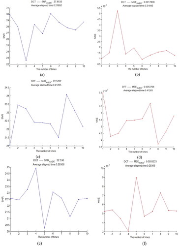
Then, average the results of 10 times of experiments, as shown in Figure 5. The effect of the DCT base is still the best and the average elapsed time is the least. The effect of the DFT base and DWT base is equivalent, but the time overhead of DFT base is the largest.

Figure 5. Average result of 10 reconstruction experiments for a frame strong earthquake signal based on three kinds of sparse bases, (a) is the signal-to-noise ratio and average signal-to-noise ratio based on DCT basis, (b) is the mean square error and average mean square error based on DCT basis, (c) is the signal-to-noise ratio and average signal-to-noise ratio based on DFT basis, (d) is the mean square error and average mean square error based on DFT basis, (e) is the signal-to-noise ratio and average signal-to-noise ratio based on DWT basis, (f) is the mean square error and average mean square error based on DWT basis.

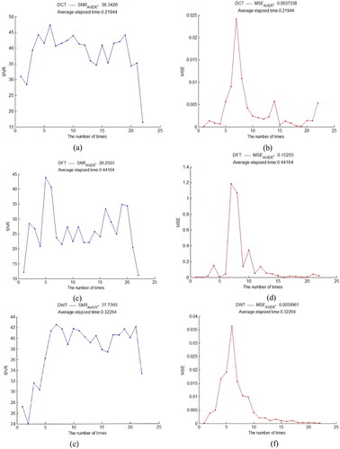
Finally, compressive sampling and reconstruction experiments are performed on a complete strong earthquake signal record. Note that there are 57 frames in the strong vibration record. The zero-noise frames which were recorded before and after the earthquake are eliminated in the selection process, and then 22 frames are left. The results of compressive sampling and reconstruction based on 3 kinds of sparse basis are shown in Figure 6 after. The DCT basis still has the best reconstruction effect and the least time consumption. The reconstruction effect of the DWT basis is close to the DCT basis. It takes more time than the DCT basis, but it is better than the DFT basis. Therefore, the DCT basis is a fixed sparse basis which is more suitable for strong earthquake signals.

Figure 6. Reconstruction experiment results of a complete strong earthquake record based on three sparse bases, (a) is the reconstructed signal-to-noise ratio and average signal-to-noise ratio based on DCT basis, (b) is the reconstructed mean square error and average value based on DCT basis, (c) is the reconstructed signal-to-noise ratio and average signal-to-noise ratio based on DFT basis, (d) is the reconstructed mean square error and average value based on DFT basis, (e) is the reconstructed signal-to-noise ratio and average signal-to-noise ratio based on DWT basis, (f) is the reconstructed mean square error and average value based on DWT basis.

4.2. Selection of measurement matrices

The applicability of Gaussian random matrix, Bernoulli random matrix, sparse random measurement matrix, part of Fourier matrix and part of Hadamard matrix to strong earthquake signals is observed in this experiment. Define the frame length N = 400 and select a frame of strong earthquake data, the fixed measurement number M = 240. Use DCT basis as the sparse base, the OMP algorithm as the reconstruction algorithm, and change the measurement matrices in the experiments.

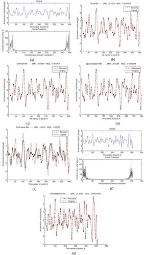
First, according to formula (5), use different measurement matrices to perform compressive sampling and reconstruction experiment on a frame of strong earthquake signal, as shown in Figure 7. It can be seen that for a single experiment, the effect of Gaussian random matrix, Bernoulli random matrix and sparse random measurement matrix are good and similar, and partial Fourier matrices are significantly worse. Partial Hadamard matrix works best, but it is required that the frame count N should be an integer multiple of two, and the frame length should be changed to 512 to complete the experiment, limiting the application range and occasion of the matrix.

Figure 7. A Single reconstruction experiment of a strong earthquake signal based on different measurement matrices, (a) is a waveform diagram of a strong earthquake signal with a frame length of 400 in the time and frequency domain, (b) is the sampling and reconstruction results based on a random Gaussian measurement matrix, (C) is the sampling and reconstruction results based on the random Bernoulli measurement matrix, (d) is the sampling and recovery results based on the sparse random measurement matrix, (e) is the sampling and recovery results based on the partial Fourier measurement matrix, (f) is the waveform diagram of the strong earthquake signal with a frame length of 512 in the time and frequency domain,(g) is the sampling and recovery results of the signal in (f) based on partial the Hadamard measurement matrix.

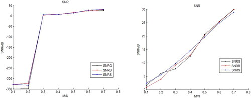
Then, the random Gaussian matrix, random Bernoulli matrix and sparse random measurement matrix are used to compare the reconstruction performance of OMP algorithm and BP algorithm under different compression ratios (M/N). In Figure 8 (a), SNRG, SNRB, and SNRS respectively represent the signal-to-noise ratio of the strong earthquake signal when the random Gaussian observation matrix, random Bernoulli observation matrix, and sparse random matrix are used. When these three kinds of matrices are used, the reconstructed strong earthquake signal-to-noise ratio increases with the increase of the compression ratio M/N, and the performance are similar. In addition, the signal-to-noise ratio of the reconstructed signal is less than 300 when the compression ratio is 0.1 and 0.2, indicating that the reconstruction error is very large, and the signal-to-noise ratio of the reconstructed signal changed a lot when the compression ratio is changed from 0.2 to 0.3. This occurs in the OMP algorithm but not in the BP algorithm, as shown in Figure 8 (b), which shows that the BP algorithm is more stable.

Figure 8. Signal-to-noise ratio curve for a frame of strong earthquake signal based on different measurement matrices and corresponding compression ratios m/n, (a) is the curve of the OMP algorithm, (b) is the curve of the BP algorithm.

4.3. Effect of compression ratio

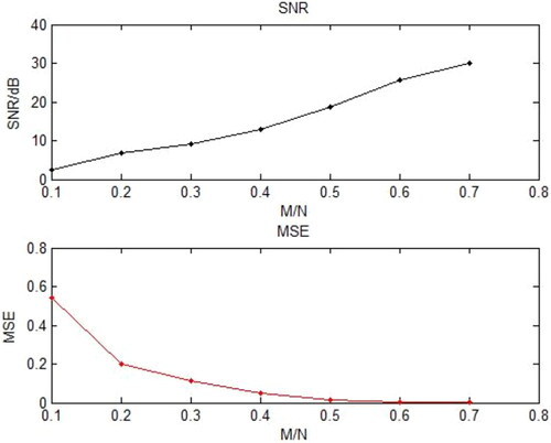
First, investigate the effect of the observation number M on the reconstruction performance by using the BP algorithm. Take 400 points as the frame length, DCT base as sparse matrix, and Gaussian random matrix as measurement matrix. M/N is taken from 0.1 to 0.7. Through the signal-to-noise ratio under different M/N, the performance of sampling and reconstruction of strong earthquake signals based on compressive sensing theory is investigated. As shown in Figure 9, with the increase of M/N, the signal-to-noise ratio increases, that is, when the frame length N is fixed, the more observation points, the better the reconstruction performance.

Figure 9. Signal-to-noise ratio curve and mean square error curve of a frame of strong earthquake signal reconstructed at different compression ratios M/N.

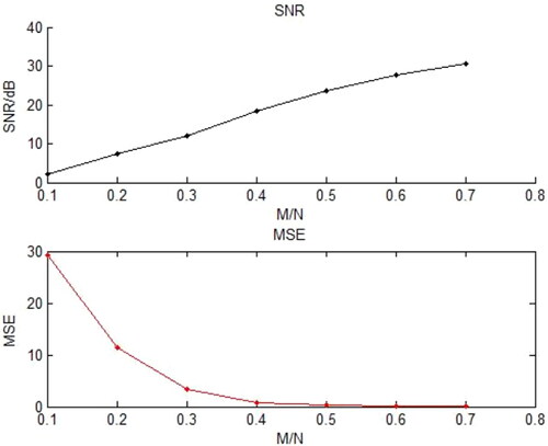
For a complete strong earthquake record, take 400 points as the frame length, DCT base as sparse matrix, and Gaussian random matrix as measurement matrix. M/N is taken from 0.1 to 0.7. Through the average signal-to-noise ratio of different frames F_AverSNR under different M/N, the performance of sampling and reconstruction of strong earthquake signals based on compressive sensing theory is investigated. As shown in Figure 10, with the increase of M/N, the signal-to-noise ratio increases, that is, when the frame length N is fixed, the more observation points, the better the reconstruction performance.

Figure 10. Average signal-to-noise ratio of different frames (F_AverSNR) curve and mean square error of different frames (F_AverMSE) curve of the complete strong earthquake record reconstructed at different compression ratios M/N.

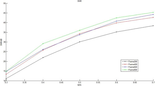
Then the BP algorithm is used to investigate the effect of frame length selection on the compressive sampling and reconstruction performance of strong earthquake signals. The signal-to-noise ratio (SNR) of the fixed frame with different frame length under different compression ratios M/N is analyzed. Take frame length as 200,400,600,800 points respectively. The results are shown in Figure 11.

Figure 11. Signal-to-noise ratio (SNR) curve of fixed strong earthquake signals with different frame lengths reconstructed at different compression ratios M/N.

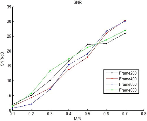
As shown in Figure 11, the number of observation and the length of frames have an effect on the reconstruction performance. When the frame length is fixed, the signal-to-noise ratio (SNR) increases with the increase of M/N.

For a complete strong earthquake record, the BP algorithm is used to investigate the effect of frame length selection on the compressive sampling and reconstruction performance. The signal-to-noise ratio (SNR) of the different frame F_AverSNR under different compression ratios M/N is analyzed. Take frame length as 200,400,600,800 points respectively. The results are shown in Figure 12.

Figure 12. Average signal-to-noise ratio of different frames (F_AverSNR) curve of a complete strong earthquake record contained by BP algorithm and reconstructed at different compression ratios M/N.

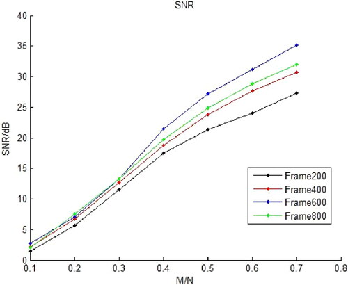
OMP algorithm is used to repeat the experiment shown in Figure 12, and the results are shown in Figure 13. From the diagram, when the frame length is fixed, the more observations, the better the reconstruction performance. However, the deviation of the F_AverSNR is too large when the compression ratio M/N ≤ 0.3, so the value of the transverse axis in the figure starts from 0.3 to 0.7. The SNR of OMP algorithm is obviously higher than that of BP algorithm; therefore, OMP algorithm is characterized by better reconstruction performance.

Figure 13. Average signal-to-noise ratio of different frames (F_AverSNR) curve of a complete strong earthquake record contained by OMP algorithm and reconstructed at different compression ratios M/N.

4.4. Reconstruction evaluation of strong earthquake records with different magnitude

Compression sampling and reconstruction of real strong earthquake records with different magnitudes and epicenter distances are performed in this section, as shown in Figure 14. The first column on the left is the original strong seismic waveform (blue) and the reconstructed strong seismic waveform (red). For better show effect, the two figures are not overlapped, and the reconstructed figure is moved to leave. The middle column is the graph of observations obtained by compressive sampling. The rightmost column is the curve of frame average signal-to-noise ratio (F_AverSNR) of a complete strong earthquake record.

Figure 14. Results of compressive sampling and reconstruction of real strong earthquake records with different magnitudes and epicenter distances. (a1) Magnitude 4.6 earthquake, epicenter 38 km (a2)(a3)Reconstruction by OMP algorithm. (b1) Magnitude 4.6 earthquake, epicenter 38 km(b2)(b3) Reconstruction by BP algorithm. (c1) Magnitude 5.1 earthquake, epicenter 57 km(c2)(c3) Reconstruction by OMP algorithm. (d1) Magnitude 5.1 earthquake, epicenter 57 km(d2)(d3) Reconstruction by BP algorithm. (e1) Magnitude 6.4 earthquake, epicenter 78 km(e2)(e3) Reconstruction by OMP algorithm. (f1) Magnitude 6.4 earthquake, epicenter 78 km(f2)(f3) Reconstruction by BP algorithm. (g1) Magnitude 7.1 earthquake, epicenter 135 km(g2)(g3) Reconstruction by OMP algorithm. (h1) Magnitude 7.1 earthquake, epicenter 135 km(h2)(h3) Reconstruction by BP algorithm.

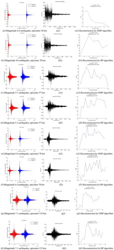
From the evaluation experiment conclusions in the previous sections, the reasonable parameter configuration that can be selected for the OMP algorithm is DCT basis and random Gaussian matrix. According to the analysis in Figure 13, the frame length N is 800 and M/N is 0.6.

For the BP algorithm, it’s the same as the OMP algorithm except that the frame length N should be 600according to the analysis in Figure 12. The reconstruction effect of the OMP algorithm is stronger than the BP algorithm, and the average signal-to-noise ratio is 9-10dB higher than the BP algorithm.

5. Conclusion

Earthquake early warning is an effective method for disaster reduction and prevention, which has developed rapidly in the world in recent years. Oriented to practical applications, this article focuses on the hot research question how to reduce the amount of data in the collection and transmission of strong earthquake signals without affecting the signal quality. The research is based on the theory of compressive sensing (CS), that is, if a signal is sparse in an orthogonal space, it can be compressed at a sampling rate much lower than the Nyquist sampling rate, and may be reconstructed with high probability. Especially it’s emphasized that the sparseness of the signal may be one of the essential conditions of compressive reconstruction. The combination of compressive sensing theory and earthquake early warning brings great convenience to the signal sampling, storage, transmission and processing. Besides, it’s the subversion of the traditional strong earthquake signal analysis method-replacing the traditional strong earthquake sampling value with the observation value in the compressive sensing theory, which will inevitably lead to a fundamental change in signal characteristics, and then affect the relevant theories and technique systems of strong earthquake signals. It is of great practical significance to apply compressive sensing in the field of earthquake early warning to explore new methods of strong earthquake signal processing. The various key technologies in compressive sensing of strong earthquake signals are the basis for its practical application.

The compressive sampling of strong earthquake signals is achieved based on compressive sensing theory, which breaks the bottleneck of the Nyquist-Shannon sampling theory to certain extent. The article first expounds the basic theory of compressive sensing, and proposes a system framework for compressive sensing of strong earthquake signals based on orthogonal basis. Then the selection of sparse basis is analyzed, and the applicability of discrete Fourier transform basis (DFT), discrete cosine transform basis (DCT), and discrete wavelet transform basis (DWT) to strong seismic signals is investigated. Then, the selection of observation matrix is discussed, and the applicability of random Gaussian matrix, random Bernoulli matrix, sparse random measurement matrix, partial Fourier matrix, and partial Hadamard matrix to strong earthquake signals is discussed. Finally, based on this framework, the base pursuit (BP) and orthogonal matching pursuit (OMP) algorithms are used to reconstruct the strong earthquake signals after being compressive sampled, and the effects are compared and analyzed. When the discrete cosine basis (DCT) and random Gaussian observation matrix are used for compressive sensing of strong earthquake signals, the frame length and compression ratio of each strong earthquake signal will affect the signal reconstruction performance. In practical applications, it is necessary to comprehensively consider parameter settings from the perspective of a combination of software and hardware.

Conflicts of interest/competing interests

There authors declared that there is no conflict of interest in the paper.

Data availability statement

The data that support the findings of this study are available from the author Jiening Xia upon reasonable request.

References

- Bajwa WU, Haupt JD, Raz GM, et al. 2007. Toeplitz-structured compressed sensing matrices. 2007 IEEE/SP 14th Workshop on Statistical Signal Processing. IEEE. 294–298.
- Baraniuk RG, Cevher V, Duarte MF, Hegde C. 2010. Model-based compressive sensing. IEEE Trans Inform Theory. 56(4):1982–2001.
- Candes EJ, Romberg J, Tao T. 2006. Robust uncertainty principles: exact signal reconstruction from highly incomplete frequency information. IEEE Trans Inform Theory. 52(2):489–509.
- Candes EJ, Romberg JK, Tao T. 2006. Stable signal recovery from incomplete and inaccurate measurements. Comm Pure Appl Math. 59(8):1207–1223.
- Candes EJ, Tao T. 2006. Near-Optimal Signal Recovery from Random Projections: Universal Encoding Strategies? IEEE Trans Inform Theory. 52(12):5406–5425.
- Chen SS, Donoho DL, Saunders MA. 2001. Atomic decomposition by basis pursuit. SIAM Rev. 43(1):129–159.
- Cooper JD. 1868. Letter to editor, San Francisco Daily Evening Bulletin. Nov. 3.
- Dang K, Ma LH, Tian Y, Zhang HW, Le R, Li XP. 2015. Construction of the Compressive Sensing Measurement Matrix Based on M Sequences. Journal of XIDIAN University. 42(02):186–192.
- Do TT, Gan L, Nguyen N, et al. 2008. Sparsity adaptive matching pursuit algorithm for practical compressed sensing. 2008 42nd Asilomar Conference on Signals, Systems and Computers. IEEE. 581–587.
- Donoho DL. 2006. Compressed sensing. IEEE Trans Inform Theory. 52(4):1289–1306.
- Efron B, Tibshirani R, Johnstone I, Hastie T. 2004. Least angle regression. Ann Statist. 32(2):407–499.
- Fang H, Zhang QB, Wei S. 2008. A method of image reconstruction based on sub-Gaussian random projection. Journal of Computer Research and Development. 45(8):1402–1407.
- Haupt J, Bajwa WU, Raz G, Nowak R. 2010. Toeplitz compressed sensing matrices with applications to sparse channel estimation. IEEE Trans Inform Theory. 56(11):5862–5875.
- Jiao LC, Yang SY, Liu F, Hou B. 2011. Development and Prospect of Compressive Sensing. Acta Electronica Sinica. 39(07):1651–1662.
- Kanamori H, Hauksson E, Heaton T. 1997. Thomas Heaton. Real-time seismology and earthquake hazard mitigation. Nature. 390(6659):461–464.
- Li S, Ma CW, Li Y, Chen P. 2013. Survey on Reconstruction Algorithm Based on Compressive Sensing. Infrared and Laser Engineering. 42(S1):225–232.
- Ma Q. 2008. Study and Application on Earthquake Early Warning. Institute of Engineering Mechanics, China Earthquake Administration, Harbin, China.
- Mallat SG, Zhang Z. 1993. Matching pursuits with time-frequency dictionaries. IEEE Transactions on Signal Processing. 41(12):3397–3415.
- Pati YC, Rezaiifar R, Krishnaprasad PS. 1993. Orthogonal matching pursuit: Recursive function approximation with applications to wavelet decomposition. Proceedings of 27th Asilomar conference on signals, systems and computers. IEEE. 40–44.
- Rosasco L, Verri A, Santoro M. 2009. Iterative projection methods for structured sparsity regularization. CSAIL Technical Reports.
- Sarvotham S, Baron D, Wakin M, et al. 2005. Distributed compressed sensing of jointly sparse signals. Asilomar Conference on Signals, Systems, and Computers. :1537–1541.
- Tropp JA, Gilbert AC. 2007. Signal recovery from random measurements via orthogonal matching pursuit. IEEE Trans Inform Theory. 53(12):4655–4666.
- Wang HT, Chen Y, Zhuang CT. 2004. Application of STEIM2 Compression Algorithm from SEED in Real Time Seismic Waveform Data Transmission. Seismological and Geomagnetic Observation and Research. 25(04):14–19.
- Wang XW, Cui GL, Wang L, Jia XL, Nie W. 2014a. Construction of Measurement Matrix in Compressed Sensing Based on Balanced Gold Sequence. Chinese Journal of Scientific Instrument. 35(01):97–102.
- Wang X, Wang K, Wang QY, Liang RY, Zuo JK, Zhao L, Zou CR. 2014b. Deterministic Random Measurement Matrices Construction for Compressed Sensing. Journal of Signal Processing. 30(04):436–442.
- Wang W, Ni S, Chen Y, Kanamori H. 2009. Magnitude estimation for early warning applications using the initial part of P waves: a case study on the 2008 Wenchuan sequence. Geophys Res Lett. 36(16):1–9.
- Xia YS, Yang LP. 2000. Study on earthquake early warning (alarm) system and benefit of disaster reduction. North Western Seismological Journal. 22(4):452–457.
- Yang ZS, Yang JQ, Yao Y. 2019. Compression Technology and Data Decompression of Seismic Exchange Standard Data. Journal of Seismological Research. 42(01):144–149.
- Zhang G, Jiao S, Xu X, et al. 2010. Compressed sensing and reconstruction with bernoulli matrices. The 2010 IEEE International Conference on Information and Automation. IEEE. p. 455–460.