Spatiotemporal shifts in thermal climate in responses to urban cover changes: a-case analysis of major cities in Punjab, Pakistan

Abstract

This study investigates the relationship of urban thermal environment (UTE) with various influential factors as well as ecological conditions. The relation between LST and land use and land cover (LULC) changes was explored in terms of remote-sensing (RS) based indices; heat effect contribution index (HECI), Urban thermal field variance index (UTFVI), Surface urban heat island intensity (SUHII), Normal Difference Built-up Index (NDBI), and Normal Difference Vegetation Index (NDVI). LULC maps were classified using the unsupervised classification technique and made error matrix to determine the accuracy. Results revealed that the vegetated area in Faisalabad decreased by 230 km² due to an expansion in the urban area of 124-320 km² during the period 1992-2014. An average LST in the rural buffers is increasing rapidly as compare to urban buffer and varied over the eight years with a range of 0.68-2.57 (°C). After 2007, SUHII's linear trend was negative because rural temperatures were still rising. Based on HECI, we found that urban expansion mainly led to increase in LST. UTFVI has shown poor ecological conditions in all urban buffers. In addition, there is a positive correlation between LST and NDBI, while NDVI indicates a negative correlation with LST.

Keywords:

• LULC
• thermal heat
• LST
• surface urban heat island intensity (SUHII)

1. Introduction

In 2018, about 55% of the world's population resides in urban areas, and by 2050 it will rise to 68% (Department of Economics and Social Affairs and U. N 2019). According to the 2018 UN Report, the urban population will rise to 2.5 billion by 2050, with Africa and Asia accounting for 90% of the population. The urbanization process has influenced the natural environment of urban areas and their services. The most disturbing effects of unplanned urbanization, combined with regional and global warming and climate change, are faced by developing countries. The LULC change is altered regionally and locally by anthropogenic activities led to change the balance of surface energy and LST (Jain et al. 2017). Changing the near-surface energy budget (inward and outward radiation) and atmospheric structure (wind speed, pressure, etc.) is the main environmental issues due to alarming increase in urbanization (Jones et al. 2008, Santamouris et al. 2018, Fan et al. 2019). Urbanization is the most visible anthropogenic force on Earth that causes phenomenon of urban heat island (UHI) and serves as the primary predictor of LULC change. The urban extension replaces the natural vegetation with impermeable surfaces, causing major changes in UTE (Wang et al. 2016, Dai et al. 2018). The related phenomenon of UHI increases urban temperature relative to rural/suburban temperatures and it is serious urban issue related to regional warming. That's why the study of LULC change from vegetation to imperious surfaces (buildings, roads) is considered in numerous urban management studies. The main focus of global studies is on these anthropogenic indicators, where they are positively linked to changes in UTE (Liu et al. 2016). Urban growth eliminates greenery and thus affects the local climate. These studies have concluded that urbanization is a potential cause for LST transition. (Li et al. 2012, Sahana et al. 2019, Ullah et al. 2019). Analysis of the LST provides valuable urban climate information and is a strong predictor of climate change. In addition to these, under these conditions, the UHI phenomenon may also have other dangerous environmental impacts that threaten the sustainable use of natural resources (Li et al. 2012, Cai et al. 2017, Peng et al. 2018, Song et al. 2018, Yamamoto and Ishikawa 2020, Zhou et al. 2020). In urban areas, the higher LST magnitude is due to impermeable surfaces that exacerbate the impact of UHI (Zhang et al. 2017). Increased LST regimes have produced an UHI. Urban cover will occupy 66 percent of the land cover globally and it boosts the LST and urban heat. (Yang et al. 2017, Cao et al. 2019). Urban LST is associated with LULC changes in tropical and sub-tropical climate regions. Built-up areas in tropical regions have a higher LST magnitude.(Li et al. 2012). Previous studies have shown that changes to the LULC have had a significant environmental effects on the regional atmosphere. (Sahana et al. 2019). In the lower Himalaya region, Pakistan, Ullah et al. (2019) have studied the relationship between LUULC changes and LST. It was concluded from this research that built-up areas had the highest LST as contrasted to the other groups of LULC (Ullah et al. 2019). Zhou et al. (2020) analyzed the composition of land cover impacts on the LST in Washington DC, America (Zhou et al. 2020). In addition, Yamamoto and Ishikawa (2020) investigated that in the high-density urban environment, LST was higher and showed high urban density in Osaka at daytime pronounced to higher LST (Yamamoto and Ishikawa 2020). NDVI and NDBI are important indicators of LULC changes (Raynolds et al. 2008, Cai and Sharma 2010). Different thermal indices (HECI, UTFVI, and SUHII) are helpful in identifying the influence of LULC changes on the increasing UTE and the environmental conditions of each city’s core region. (Liu and Zhang 2011, Zhou et al. 2014, Huang, Huang et al. 2019, Renard et al. 2019).

However, due to the spatial scarcity and lack of consistent distribution of existing on-site stations, especially in developing countries such as Pakistan, accurate estimation of changes in SUHII is challenging. Under these conditions, RS datasets provide a rare opportunity to test these phenomena arising from LULC changes. RS technology has become a critical instrument for retrieving the LST with the steady production of sensors (Cai et al. 2017, Peng et al. 2018, Song et al. 2018). As a result of LULC changes, RS techniques were used to assess the spatiotemporal changes in human-induced urban climate phenomena (SUHII) (Cai et al. 2017, Peng et al. 2018, Song et al. 2018, He et al. 2019). Studies have stated that thermal infrared RS data has been commonly used to investigate the SUHII effects by retrieving LST (Li et al. 2011). Satellite images were used to find UHI and thermal environment influencing variables in urban areas to measure the effect of LULC shifts on the UTE (Guha et al. 2018). RS powered LST, for example, ASTER and MODIS, have been used to examine thermal changes in an urban area (Liu and Zhang 2011, Zhou et al. 2014). The major limitations of ASTER and MODIS data in the current study are that their resolutions for analyzing UTE on a city scale are comparatively coarse.

There are previous studies have been published on the thermal evaluation of the Punjab Plain urban areas (land drained by the Indus River and its tributaries), focusing on the city's single-core urban agglomeration zone, and little attention has been paid to identifying factors contributing to increase LST and SUHII phenomena. Arshad et al. (2019) studied the impact of LULC changes on the regional climate of Faisalabad and concluded that urban cover caused higher regional temperature (Arshad et al. 2019). Sajid, Ahmad, and Javed (2020) have considered the NDVI as a LULC change factor to know the urban contribution to LST of Lahore, Faisalabad, and Multan cities in Pakistan (Sajid, Ahmad, Javed 2020). Sadiq Khan et al. (2020) studied the anthropogenic influences on urban climate by considering urbanization and concluded it has affected the LST pattern in capital city of Pakistan (Sadiq Khan et al. 2020). Previous studies performed based on particular environmental factors for a single city. For instance, RS data was used in Lahore city to study land use activities and LULC changes that intensified the SUHII (Shah and Ghauri 2015). Still, few studies have been reported in context to indentify driving factors of UTE. Current study, quantifies the UTE driving mechanism by integrating the multi factors including (HECI, UTFVI, SUHII, NDBI, and NDVI) to evaluate the impact of individual LULC changes on UTE and ecological condition of major cities of Punjab. Pakistan is highly exposed to climate change and faced major extreme events, in order to follow the UN sustainable goals and there is significant need to make sustainable urban cities. In recent years, extensively LULC changed in the major cities of Punjab and affected the regional/local urban climate that causes heatwaves, diseases, social life disturbance (Sadiq Khan et al. 2020; Arshad et al. 2019).

In this study of land-use transition drivers (NDVI/NDBI) and their potential impacts on the UTE, there is also a significant environmental issue involved. To facilitate the analysis, the RS based LST and various heat indices (SUHII, HECI, and UTFVI) were used . In the current research, RS dataset (Landsat) has been used to study the UTE and to measure LULC shifts, particular attention has been paid to the buffer zones (rural and urban areas). This research attempted to investigate and quantify the LULC changes and particularly their contributions to the intensification of UTE. Additionally, in six major cities of Punjab, Pakistan, the driving factors of UTE were investigated in terms of SUHII, HECI, UTFVI, and their effects on local ecological conditions.

This research therefore seeks to examine the changes in long-term land cover and their impacts on the UTE. RS based estimation offers real-time spatiotemporal changes in LST (Zhou et al. 2014, Zhou et al. 2018). Landsat products with a resolution of 30 m are currently suitable for study of spatial changes in LST and LULC in the major cities. In major towns, RS retrieved LST is a convenient source to examine the SUHII and its supporting factors. Landsat have different missions and their spatiotemporal resolutions and bands information as shown in Tables 1 and 2.

Table 1. Satellite bands details from 1992 to 2014.

No	Acquisition date				Path/row
	Landsat5	Landsat5	Landsat7	Landsat8
1	1992-06-16	1999-06-20	2007-06-01	2014-06-29	150/38
2	1992-07-02	1999-07-06	2007-07-20	2014-07-15	150/38
3	1992-08-11	1999-08-23	2007-08-05	2014-08-16	150/38
4	1992-09-20	1999-09-08	2007-09-15	2014-09-17	150/38
5	1992-10-06	1999-10-26	2007-10-24	2014-10-03	150/38
6	1992-11-23	1999-11-11	2007-11-07	2014-11-20	150/38
7	1992-12-09	1999-12-13	2007-12-27	2014-12-06	150/38
8	1992-06-09	1999-06-13	2007-06-11	2014-06-22	149/38
9	1992-07-05	1999-07-09	2007-07-29	2014-07-08	149/38
10	1992-08-11	1999-08-16	2007-08-30	2014-08-25	149/38
11	1992-09-29	1999-09-21	2007-09-06	2014-09-26	149/38
12	1992-10-31	1999-10-03	2007-10-17	2014-10-12	149/38
13	1992-11-16	1999-11-20	2007-11-18	2014-11-13	149/38
14	1992-12-02	1999-12-22	2007-12-04	2014-12-15	149/38
15	1992-06-16	1999-06-20	2007-06-01	2014-06-29	150/39
16	1992-07-02	1999-07-06	2007-07-20	2014-07-15	150/39
17	1992-08-11	1999-08-23	2007-08-05	2014-08-16	150/39
18	1992-09-20	1999-09-08	2007-09-15	2014-09-17	150/39
19	1992-10-06	1999-10-26	2007-10-24	2014-10-03	150/39
20	1992-11-23	1999-11-11	2007-11-07	2014-11-20	150/39
21	1992-12-09	1999-12-13	2007-12-27	2014-12-06	150/39

Table 2. Accuracy evaluation of the LULC maps for 1992, 1999, 2007, and 2014.

LULC	Years
	1992	1999	2007	2014
Water	0.80	0.83	0.87	0.82
Urban	0.81	0.83	0.88	0.89
Vegetation	0.87	0.80	0.82	0.85
Other	0.82	0.82	0.87	0.81
Overall accuracy	0.86	0.87	0.86	0.87

The objective of this analysis is threefold: (i) to examine the changes in the long-term perspective of LULC and its indicators (NDVI and NDBI); (ii) to compute the different heat indices (SUHII, HECI and UTFVI) to describe the urban thermal phenomenon in urban areas; (iii) to evaluate the possible impacts on LST of the various LULC drivers. Landsat Products (Landsat 5 (TM); Landsat 7 (ETM+) and Landsat 8 (OLI/TIR) were used for LULC changes, NDVI, NDBI and LST (e.g., SUHII, HECI and UTFVI) modifications. This research provides a real understanding of UTE’s relationship with various influential factors and SUHII’s long-term pattern, as well as the environmental conditions in the major cities.

2. Materials and methods

2.1. Study area

Punjab is Pakistan’s second largest province, with a total surface area of about 205344 km². The study area consists of major cities, which are Faisalabad, Lahore, Gujranwala, Multan, Sargodha, and Sialkot, as shown in Figure 1 and Table 3. The name Punjab comes from the presence of five rivers: Indus, Chenab, Ravi, Jhelum, and Sutlej, which means that it is fertile for agriculture. There is a subtropical climate in the Punjab that is characterized as mild, humid in summer and cold in winter. The average annual rainfall is 600 mm in the northwest, based on 22 years of historic metrological measurements. From June to September, there is a rainy season called the monsoon season. Temperature changes from −2 to 45 °C, on the other hand, but maximum and minimum temperatures exceed 47 °C and −5 °C, respectively. The Punjab province was facilitated by 300 irrigated channels. Punjab has played a leading role in Pakistan economic and social development. In Pakistan’s economic and social growth, Punjab has played a leading role. It is one of Pakistan’s fastest-growing provinces, especially in terms of growth, urbanization, population, and agricultural development. It is named the country’s lifeline and the topography of Punjab is plain. The topographic elevation falls from 2271 m in the north to 46 m on the south side. Meanwhile, due to rapid urbanization, many urban and regional thermal problems have emerged in Punjab.

Figure 1. Study Area and buffer’s information.

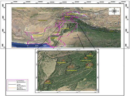
Table 3. Populations and Population density of the six major cities, of Punjab, Pakistan. (Source: Statistics (2017).

No.	Cities	Area km^2	Population Thousand per person			Population Density km^-2
			1981	1998	2017	1981	1998	2017
1	Lahore	1772	3545	6319	11126	2001	3566	6279
2	Faisalabad	5856	3562	5430	7874	608	927	1345
3	Gujranwala	3622	2108	3401	5014	582	939	1384
4	Multan	3700	1970	3117	4045	530	838	1276
5	Sialkot	3016	1803	2723	3894	598	903	1291
6	Sargodha	5854	1912	2666	3704	327	455	633

To accomplish urban planning goals, it is therefore important to understand UTE's spatiotemporal pattern. Two zones (urban and rural) were established in this study to evaluate the impact of LULC changes on UTE. The drawing buffers around the metropolitan cities (Faisalabad, Lahore, Gujranwala, Multan, Sargodha, and Sialkot) provide a schematic distinction between rural and urban sites based on land cover. For the creation of urban and rural scenarios, each city is marked with two buffers at different radii, as well as their Koppen-Geiger zone designation, as shown in Table 3. Two concentric buffers were selected in the way that the inner buffer mainly having the urban cover and less vegetation load and it is called "urban buffer". The center of buffers is same as center of city. The outer buffer is considered to be 'rural' based on the vegetation cover and is marked with twice the radius of the inner buffer to take into account the effects of the rural location, including trees, rural land etc. Compared to the urban buffer, the rural buffer has less infrastructure and consists of bulk vegetation load. Also, local characteristics, such as LST patterns, wind speed shift, and urban growth rate, were taken into count to determine extent and shape of buffers.

2.2. Data collection and preprocessing

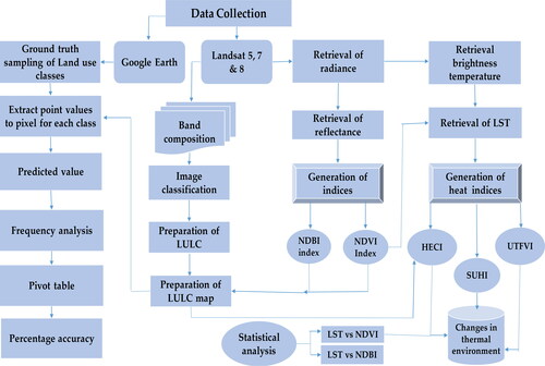
Based on remotely sensed LST and various heat indices, this study examined the long-term LULC changes and their influences on the thermal climate. Data derived from various Landsat products (Landsat 5 Themetic Mapper (TM), Landsat 7 Enhanced Themetic Mapper (ETM+) and Landsat 8 Operational Land Imager (OLI / TIRS) were acquired from the U.S. Geological Survey (USGS https:/earthexplorer.usgs.gov/) for the period 1992 to 2014 at a time resolution of 16 days and a spatial resolution of 30 m shown in Table 1. All spectral bands were acquired by < 10% clouds and atmospheric corrections were performed in the ENVI programme using the radiometeric correction toolbox. To correct atmospheric errors and eradicate atmospheric influences, the FLAASH atmospheric correction model was used from the atomspheric correction module to obtain accurate surface characteristics of bands including thermal, visible, near-infrared, and shortwave infrared bands(Matthew et al. 2000). The spectral bands (thermal, visible, near-infrared, and shortwave infrared) were used for the measurement of the LULC changes and LST after all corrections. To derive NDVI, NDBI, and LST, the digital number of the spectral bands was translated into radiance and finally into reflectance value. (Chen et al. 2006, Pan 2016). In the following steps, the detailed procedure of radiance derivation and then LST is defined and also shown in Figure 2. Based on various heat indices, i.e., SUHII, UTFVI, and HECI, the retrieved LST was further used to evaluate changes in the thermal environment.

Figure 2. Flow diagram of data preprocessing and analysis scheme.

1. Digital numbers of spectral bands were firstly converted into spectral (TOA) radiance (L _λ) using the formula (Pan 2016). (1) $$\mathrm{L}\mathrm{\lambda }=\mathrm{ }{\frac{{\mathrm{L}}_{\text{maxλ}}-{\mathrm{L}}_{\text{minλ}}}{\left({\mathrm{Qcal}}_{\text{max}}-{\text{Qcal}}_{\text{min}}\right)}\times (\mathrm{Qcal}}_{\text{max}}-{\text{Qcal}}_{\text{min}})+ {\mathrm{L}}_{\text{minλ}}$$(1) (2) $$\mathrm{L}\mathrm{\lambda }=M_L\mathrm{ }{Q}_{\mathit{cal}}+A_L$$(2) where ${\mathit{L}}_{\mathit{\lambda }}$ = Spectral radiance $(\mathit{Watt} m^{-2}{sr}^{-1}\mu m^{-1}),$ ${\mathit{Q}}_{\mathit{cal}}$ = Pixel values in DN, ${\mathit{Q}}_{\mathit{max}}$ = Maximum Quantized calibrated pixel value (Ullah, Tahir et al.), ${\mathit{Q}}_{\mathit{min}}$= Minimum Quantized calibrated pixel value (Ullah, Tahir et al.), ${\mathit{L}}_{\mathit{max}}$ = Spectral radiance scaled to Q_max, and ${\mathit{L}}_{\mathit{min}}$ = Spectral radiance scaled to Q_min, and M_L = Radiance multi band, A_L = Radiance add band.

2. Spectral bands after radiance converted into reflectance following relations: (3) $$r=\frac{\pi \times L_{\mathrm{\lambda }}\times r^2}{E_{\mathit{sun}}\times \hspace{0.17em}\text{Cos}\hspace{0.17em}\mathrm{ø}\times dr}$$(3) where $r$ = Planetary reflectance (dimensionless),$L\mathrm{\lambda }$ = Spectral radiance at the sensor aperture (watt m⁻² ster⁻¹ μm⁻¹), and $dr$ = Inverse square of earth-sun distance (astronomical unit): (4) $$\mathrm{dr}=1\mathrm{ }+\mathrm{ }0.033\text{Cos }(\mathrm{D}\mathrm{ }\times \mathrm{ }2\mathrm{ }\times \mathrm{ }3.14)/365)$$(4) where D = Day of the year, E_sun = Mean solar atmospheric irradiance $(\mathit{Watt} m^{-2}\mu m^{-1}$) $\mathrm{\theta }$=solar zenith angle (degree), θ = (90 - B), and B = Sun elevation angle. Information regarding all constant parameters took for NIR and RED bands from the LANDSAT metadata header file.

2.3. LULC maps preparation

To make LULC maps for the years 1992, 1999, 2007, and, 2014 high-resolution Landsat images from the U.S. Geological Survey (USGS) were used. Necessary area of study extracted from Landsat (5, 7, and 8) images and false-colored images produced by layer stacking of all Landsat visible, near-infrared and shortwave infrared bands in ARDAS Imagine (Shalaby and Tateishi 2007, Karakus et al. 2014, Karakuş 2019). After this, unsupervised classification technique, the ISODATA clustering algorithm was used to classify the pixels into four different land-use classes (Asmala 2012). For different LULC types, spectral signatures were defined on the basis of the spectral characteristics of Landsat imagery. To reclassify the option to recode the land-use classes, ArcGIS was used. The following four forms of land cover were categorized: urban (buildings and roads); vegetation (farmland, rural land, woodland and grassland); other (rocky land, barren land) and water (canals, rivers and pools). Landsat based NDVI and NDBI indices were used to recode LULC maps to optimize land cover information to enhance the data of each land-use category in LULC maps. In addition, the comprehensive protocol for accuracy evaluation was addressed in sections 2.3.1, 2.3.2, and 2.3.3.

2.3.1. Accuracy assessment

In ArcGIS 10.3, the accuracy assessment protocol for LULC maps was carried out. For each class, we randomly collected 100 pixels from random locations on Google Earth each year (Li et al. 2012, Zhang et al. 2013) and followed previously published literature and expert knowledge (Yuan et al. 2005, Gorelick et al. 2017, Arshad et al. 2019). In order to test their accuracy using various tools in ArcGIS software, the pixel values in the image were compared with the ground truth samples for each land-use class. The frequency analysis and error matrix using ArcGIS 10.3 (Figure 2) calculated the accuracy percentage. For the years 1992, 1999, 2007 and 2014, the average classification accuracy was 0.8683, 0.8740, 0.8639 and 0.8719, respectively, as shown in Table 2.

2.3.2. Retrieval of NDVI

NDVI can be defined as a relative greenness measurement (Raynolds et al. 2008), and NDVI is commonly used to indicate the degree of vegetation cover to differentiate between various types of vegetation and non-vegetated areas. Using the following expression, NDVI can be extracted from the reflectance value of RED and NIR bands (computed in section 2.2). (Balaghi et al. 2008, Cai and Sharma 2010, Dempewolf et al. 2014). (5) $$\mathit{NDVI}=\frac{\mathit{NIR}\mathrm{ }-\mathrm{ }\mathit{RED}}{\mathit{NIR}+\mathit{RED}}$$(5)

NDVI value is in a range between −1 and +1(Landsat 2016).

2.3.3. Retrieval of NDBI

NDBI is a built-up land spectral response. In the middle infrared band, built-up phenology typically has a greater reflectance level than the near-infrared band. It can be defined as the NDBI index; it is the fractional relation between the SWIR1 and NIR band difference to the sum of these two bands. NDBI is a very useful index of modernization to find out the changes in settlements/urban areas. Using the following relationship, NDBI will recover.(Ahmed 2018). (6) $$\mathit{NDBI}=\frac{\mathit{SWIR}1-\mathit{NIR}}{\mathit{SWIR}1+\mathit{NIR}\mathrm{ }}\mathrm{ }$$(6)

Some studies have concluded that the NDBI index showed dry vegetation has high reflectance value in the SWIR1 wavelength range and NIR wavelength range. Consequently, the calculated information about the built-up mixed up with vegetation noise. It was removed using Equation 6(6) $$\mathit{NDBI}=\frac{\mathit{SWIR}1-\mathit{NIR}}{\mathit{SWIR}1+\mathit{NIR}\mathrm{ }}\mathrm{ }$$(6) (He et al. 2010). (7) $$\mathit{Vegetation}\mathrm{ }\mathit{Noise}=\mathit{NDBI}-\mathit{NDVI}$$(7)

2.4. Retrieval of LST

In this study, LST was derived from thermal bands of Landsat products using the methodology recommended by (Sekertekin et al. 2016) and (Landsat, Landsat 2016). The following steps were adapted to retrieve LST.

1. Conversion from DN to radiance

2. Calculation of brightness temperature

3. Retrieval of LST

The first digital number of the thermal spectral bands was converted into radiance (${\mathit{L}}_{\mathit{\lambda }})$ as already described in Section B. In the second step, the radiance of the thermal spectral bands was converted into brightness temperature (TB) using the following relation (Landsat 2016), (Kumar and Shekhar 2015). (8) $$TB=\frac{K_2}{ln\mathrm{ }\left[\left(\frac{K_1}{L_{\lambda }}\right)+1\mathrm{ }\right]}$$(8) where, K1 and K2 are the conversion constants, $L_{\lambda }$ is a spectral radiance and T is brightness temperature. For Landsat8 (TIRS), K1 = 774.89 $mW/{cm}^2/sr/\mu m$ and K2 = 1321.08 Kelvin, for Landsat7 (ETM+), K1 = 666.09 $mW/{cm}^2/sr/\mu m$ and K2 = 1282.71 Kelvin; Landsat5, K1 = 607.76 $mW/{cm}^2/sr/\mu m$ and K2 = 1260.56 Kelvin.

In the third step, the LST was derived using the following relation (Weng and Lu 2008). (9) $$\mathit{LST}=\frac{T_B}{1\mathrm{ }+\left(\frac{\lambda \mathrm{ }{T}_B}{\rho }\right)\ln ϵ}$$(9) where $\lambda \approx 11.5\mathrm{\mu }\mathrm{m}$ is the effective wavelength of the thermal band. $P=\frac{ hc}{\sigma }=1.438\times {10}^2 mk,$‘σ’ is the Boltzmann constant ${(1.38\times 10}^{-23} J{K}^{-1}) ,$ ‘h’ is Planck constant ${(6.626\times 10}^{-34} Js)$ and c is the speed of light ${(3.0\times 10}^8 m{s}^{-1}),$ ϵ is the land surface emissivity with 0.95, 0.92, and 0.9925 for vegetation, built-up, and water surfaces, respectively (Nichol 1994).

Land surface emissivity ($Ɛ$) was estimated using the NDVI thresholds method as proposed by (Sobrino et al. 2004) according to the equations. (10) $${\mathrm{ }d\mathrm{ }}_{\mathrm{Ɛ}}=\left(1_{-}{\mathrm{Ɛ}}_s\right)\times \left(1-p_v\right)+{F\times \mathrm{ }\mathrm{Ɛ}}_V$$(10) where ${\mathrm{Ɛ}}_v=\mathit{vegetation}\mathrm{ }\mathit{emissivity},\mathrm{ }{\mathrm{Ɛ}}_s=\mathit{the}\mathrm{ }\mathit{soil}\mathrm{ }\mathit{emissivity},$ F = shape factor and its value if 0.55 (Lim et al. 2012), $P_v=\mathit{vegetation}\mathrm{ }\mathit{proportion}$ and it was obtained according to equation (Quintano et al. 2015). (11) $${\mathrm{ }P}_v\mathrm{ }={\left(\frac{\mathit{NDVI}-{\mathrm{ }\mathit{NDVI}}_{\mathit{min}}}{{\mathit{NDVI}}_{\mathit{max}}\mathrm{ }-\mathrm{ }{\mathit{NDVI}}_{\mathit{min}}}\right)}^2$$(11)

Land surface emissivity was retrieved using the following relation: (12) $$\mathrm{Ɛ}=\left({\mathrm{Ɛ}}_{\mathrm{s}}\times P_v\right)+{\mathrm{Ɛ}}_s\left(1-p_v\right)+d_{\mathrm{Ɛ}}\mathrm{ }$$(12)

2.5. Analysis of changes in urban thermal environment (UTE) factors

Changes in the thermal environment of the six major cities were assessed in sections using RS-based derived distinct heat indices (SUHII, UTFVI, and HECI). 2.5.1, 2.5.2, and 2.5.3.

2.5.1. Surface urban heat island intensity (SUHII)

SUHII is known as the urban buffer and rural buffer temperature difference. In this research, in the form of circles around the major cities, urban and rural buffers were marked. With the aid of the following equation, SUHII was computed from average LST using the method recommended (Zhang et al. 2010). (13) $$\mathit{SUHII}=T_u-T_r$$(13)

In the above equation, ${ T}_u$ is the temperature of an urban buffer (°C) and ${ T}_r$ is the temperature of a rural buffer (°C). The average annual value of LST for the urban and rural buffer calculated by extracting LST pixels values from 1992 to 2014.

2.5.2. Urban thermal field variance index (UTFVI)

The effect on urban heat intensity of changes in underlying surfaces as measured by the UTFVI. UTFVI was used in this analysis to measure the UHI phenomenon by using the equation below(Liu and Zhang 2011). (14) $$\mathrm{U}\mathit{TFVI}=\frac{T_s-T_{\mathit{mean}}}{T_s}$$(14)

Where, UTFVI is the variance index of the urban thermal field; T_s is the temperature (LST) of the certain pixel and T _mean is the mean temperature (LST) of the whole region in (°C). UTFVI shows the spatial variation and ecological assessment of urban heat over a certain region. According to the six basic ecological assessment indices and heat island indices, UTFVI has been divided into different classes. The greater urban heat intensity and the worse state of the ecological ecosystem are indicated by a higher UTFVI value.

2.5.3. Heat effect contribution index (HECI)

Different LULCs contribute differently to the thermal environment. In this analysis, four major land covers (water, urban, vegetation, and others) that have been significantly linked to changes in LST and SUHII were taken into account. HECI was introduced and used to measure the heat contribution of various types of LULCs in the current research (Li et al. 2015). The HECI computed as, (15) $${\mathit{HECI}}_i=\frac{\sum _{j=1\mathrm{ }}^{N_i}{T}_{ij}\mathrm{ }}{\overline{T}N\mathrm{ }}\times 100\mathrm{\%}\mathrm{ }$$(15)

Where$,{ \mathit{HECI}}_i$ represents heat contribution by ${\mathit{LULC}}_i,$ its value will be from 0 to 100%. $N_{i }$ Pixel number of the area that covered by${\mathit{LULC}}_i.$$T_{ij}$ is the LST of ${\mathit{LULC}}_i$ in its $j^{th}$ pixel. $\overline{T}$ is the mean temperature of the whole area and N the total number of pixels within the area. The sum of HECI all types of LULC should be 100%.

2.6. Statistical analysis

In statistical analysis, the association between LST and NDVI, NDBI, has been found using the Piecewise Linear Regression (PWLR) model based on a piecewise linear function. From 1992 to 2014, the correlation coefficient between NDVI-LST and NDBI-LST for all major cities in Punjab, Pakistan was developed using the PWLR model.

Following relations used: (16) $${\mathrm{ }y}_{i1}=a_1+k_1\times x_{i1}$$(16) (17) $$y_{i2}=\mathrm{ }{y}_{i1}+k_2\times \left(x_{i2}-x_{i1}\right)\mathrm{ }\left\{if\mathrm{ }x{\mathrm{ }\le \mathrm{ }x}_{i1\mathrm{ }}\right\}$$(17) (18) $$y=a_1+k_1\times x\mathrm{ }\left\{\mathit{else}\mathrm{ }if\mathrm{ }x<\mathrm{ }{x}_{i2}\right\}$$(18) (19) $$\mathrm{y}=\mathrm{ }{y}_{i1}+k_2\times \left(x-x_{i1}\right)$$(19)

In the above equations, $a_{1 }$ is the intercept of the line, $k_2 \mathit{and} k_1$ are the slope of a line, and $x_{i1} \mathit{and} x_{i2}$ are the intersectional points. ANOVA one-way statistical test was used to calculate the different parameters including a significant level (95% C.I.) between NDBI/NDVI and LST. In the spatial analysis, long term spatial variations in LST and urban thermal field variance were measured using Kriging interpolation technique in ArcGIS (Yang et al. 2004). Kriging technique usually measures the spatial autocorrelation among the points and changes weight regarding the spatial allocation of sampled points (Goovaerts 1997).

3. Results

3.1. Spatial-temporal changes in LULC (1992–2014)

Four groups of LULC maps were classified: vegetation, urban, water, and others. The ground truth data obtained from Google Earth and available literature were also correlated with these LULC categories. According to Table 2, it displayed the average value of the percentage accuracy of all land use groups. LULC varies dramatically inside the marked buffers with different radii. According to Tables 3 and 4, based on their level of growth and gross domestic product (GDP), buffers/circles across all six cities were labelled with different radii. In all cities, a vegetated area is the prevailing land use cover for the current study area. The extensive modifications, primarily vegetation to transitional urban land resulting from the formation of infrastructure and roads, include vegetated cover (Figure 3). The extension of continuous urban territory, examining the land changes in detail the territory km² variations within vegetated land. The most important growth in all Punjab cities (marked buffers) was found in the artificial surface expansion from 1992 to 2014. During 1992-2014, vegetated areas were reduced to 230 km², 91 km², 553 km², 89 km², 35 km², and 64 km² in total. Besides, urban areas increased to 195 km², 67 km², 602 km², 102 km², 37 km², and 58 km² in the all cities: Faisalabad, Gujranwala, Lahore, Multan, Sargodha, and Sialkot are shown respectively in the Table 5. Vegetated areas have typically led to urban areas and other land areas in order to satisfy the demand for development and population growth, etc. Consequently, the urban area expends with the reduction of vegetated cover. The reduction of vegetated land, due to the shift to artificial areas, townships, factories, and highways, also stands out in this type of land use sector. The metropolitan area is rising dramatically in all the buffers. In addition, during the study period, other areas were also expanded. It is indicated that the vegetated land has been lost and all cities have acquired urban areas. In addition, during the study period, other areas were also expanded.

Figure 3. Land cover changes (km²) within marked buffers in selected cities from 1992 to 2014.

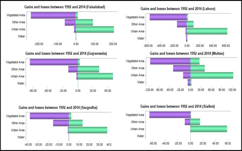
Table 4. Buffer zones marked around the Cities at different radii.

Cities	Radius of urban buffer (km)	Radius of rural buffer (km)	Koppen-Geiger Zone Classification
Faisalabad	8	16	Bwh (semi-arid climate)
Lahore	10	20	Bsh (Mid-Latitude Steppe and Desert Climate)
Gujranwala	5	10	Bsh (hot semi-arid climate)
Multan	6	12	Bwh (Tropical and Subtropical Desert Climate
Sargodha	3	6	Bwh (semi-arid climate)
Sialkot	3	6	Cwa (humid subtropical hot summer)

Table 5. LULC change matrix 1992–2014 in km².

City	LULC Type	1992	1999	2007	2014	Transferred Area (km^2)
FSD	Water	0.052	3.654	0.574	1.881	1.828
	Urban	124.76	197.81	236.62	320.04	195.28
	Other	67.421	107.78	104.91	101.12	33.72
	Vegetation	609.14	492.22	459.34	378.34	−230.79
GRW	Water	0.898	1.179	0.937	1.173	0.274
	Urban	57.36	70.65	94.27	124.89	67.535
	Other	20.85	55.56	24.67	44.92	24.074
	Vegetation	233.22	184.94	192.45	141.34	−91.884
LHR	Water	14.250	10.890	7.458	11.80	−2.446
	Urban	264.92	582.56	783.78	867.78	602.86
	Other	158.92	174.53	139.42	112.49	−46.425
	Vegetation	810.92	481.02	318.35	256.93	−553.99
MUL	Water	9.498	3.8222	5.989	5.041	−4.456
	Urban	116.15	156.95	173.63	218.75	102.6
	Other	57.829	52.30	48.20	49.44	−8.423
	Vegetation	289.63	260.02	245.28	199.9	−89.72
SGD	Water	0.093	0.025	0.058	0.325	0.232
	Urban	24.06	46.94	57.35	61.24	37.17
	Other	16.90	18.90	13.18	15.25	−1.653
	Vegetation	71.71	46.94	42.18	35.95	−35.75
SKT	Water	0.068	0.006	0.050	0.190	0.122
	Urban	10.44	17.54	47.78	68.75	58.30
	Other	9.745	6.735	10.96	16.05	6.311
	Vegetation	92.08	88.05	53.54	27.34	−64.73

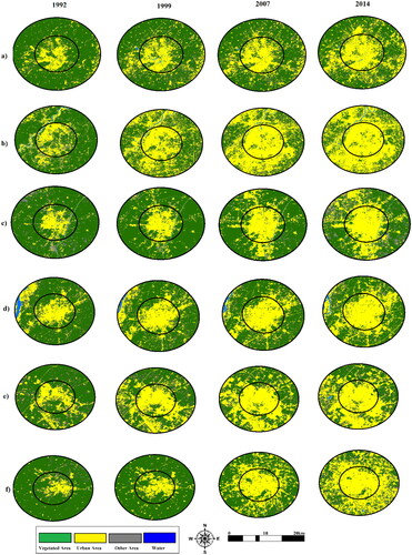
For example, the Faisalabad buffer LULC changes showed that the urban area was 124 km² in 1992, increased to approximately 197 km² in 1999, then expanded to 236 km² in 2007, and to 320 km² in 2014. Figure 4 ensured that urban extension was established in all cities, particularly in both buffers (urban and rural) after 1999. The urbanization factor continued to increase and the internal buffer named urban buffer building areas continued to expand. Owing to the growing population and migration of people to towns, even the vegetated areas and water areas of the rural buffer around the urban buffer in all towns are accompanying them. In both buffers (urban and rural), with the exception of Multan and Gujranwala in 2014, Faisalabad, Lahore, Sialkot, and Sargodha have almost full urbanization capacity. It is clearly evident that LULC changes were very noticeable in the study sites inside the buffers and how urbanization increased spatially with the period depicted in Figure 4. It is strongly evident that in the study sites within the buffers, LULC changes were very visible and how the urbanization was increasing spatially with time.

Figure 4. Spatiotemporal patterns of land cover changes for 1992, 1999, 2007 and 2014 in six major cities: (a) Faisalabad (FSD), (b) Lahore (LHR), (c) Gujranwala (GRW), (d) Multan, (e) Sargodha (SGD) and (f) Sialkot (SKT).

3.2. Spatial-temporal changes in LST (1992–2014)

From 1992 to 2014, the mean annual LST spatial variation in six major cities was extracted. Figure 5 shows the changes in annual average LST in selected cities for 1992, 1999, 2007, and 2014, showing that SUHII is heading towards the rural buffer due to the rapid expansion of urbanisation out of the urban buffer. From LST's spatial pattern, it can be inferred that the urban buffer for the UHI effect was a highly pronounced area. Results also showed that during the 1992-2014 study period, the average annual LST in rural buffers increased faster than the urban average annual LST in Faisalabad, Lahore, Multan, and Sargodha over eight years, with a difference of 0.1 °C, 0.53 °C, 0.11 °C, and 0.31 °C. The shift in the gradient of mean LST from 1992 to 2014 is seen in Figure 6 and LST was observed to increase the urban buffer's inward direction in all cities. It takes the same direction as spending in the urban region.

Figure 5. Spatial patterns of mean annual (LST) (24 °C–39 °C ) 1992, 1999, 2007, and 2014 in six major cities: (a) Faisalabad (FSD), (b) Lahore (LHR), (c) Gujranwala (GRW), (d) Multan, (e) Sargodha (SGD) and (f) Sialkot (SKT).

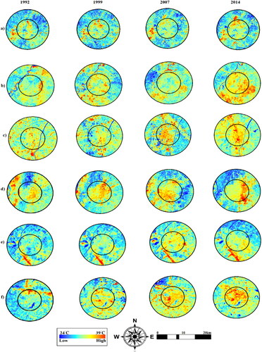
Figure 6. Change in mean annual LST from 1992 to 2014.

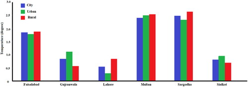
In a rural buffer, the gradient of mean LST became higher due to urban sprawl towards rural buffer. In contrast to rural areas, urban areas recorded higher temperatures. Average changes in LST over eight years in rural and urban buffers showed that mean LST increased at a rate of 1.79 °C, 0.84 °C, 0.56 °C, 2.39 °C, 2.46 °C, and 0.81 °C, in Faisalabad, Gujranwala, Lahore, Multan, Sargodha, and Sialkot, respectively. Results have suggested separately that an average LST shift every eight years has risen by 1.75 °C, 1.11 °C, 0.30 °C, 2.46 °C, 2.30 °C, and 0.94 °C, in urban buffers. Mean LST in rural buffers increased over eight years in Faisalabad, Gujranwala, Lahore, Multan, Sargodha and Sialkot, respectively, by 1.85 °C, 0.57 °C, 0.83 °C, 2.57 °C, 2.61 °C, and 0.68 °C over eight years (Figure 7).

Figure 7. Mean LST (°C) changes over eight years in urban, rural, and whole buffer.

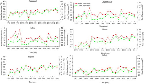
Urban expansion, particularly in these cities occurred by transforming vegetation into urban areas that changed physical surface processes and led to an increase in LST shown in Figure 8.

Figure 8. Mean annual temporal changes in LST (°C) changes over rural and urban buffer.

3.3. Spatial-temporal changes in LST (1992–2014)

Using different heat indices, remotely sensed LST was further used to examine deep thermal environmental changes, a thorough description is given in Sections 3.3.1, 3.3.2 and 3.3.3.

3.3.1. Changes in surface urban heat island intensity (SUHII)

By measuring the difference between the urban and rural buffer LST, SUHII was extracted. For the six major cities of Punjab from 1992 to 2014, Figure 9 shows the annual variations in SUHII. SUHII increased from 0.72 °C to 1.70 °C in Gujranwala city from 1992 to 1999, decreased to 0.51 °C in 2007 and then increased to 0.62 °C in 2014. All cities indicated a fluctuating pattern in SUHII from 1992-2014. The results showed that there was a positive growth trend in SUHII cities from 1999 to 2007, while the SUHII pattern shifted towards negative values after 2007.

Figure 9. Long-term annual temporal changes in (SUHII) °C in six major cities from the period of 1992-2014.

The probable explanations are that urbanisation incraesed more rapidly during 2007-2014, and definitely transformed the vegetated region into an urban one, eventually causing the high temperature of the rural buffer. Due to an increase in LST in rural buffers, the temperature differential between buffers decreased, leading to a decrease in SUHII from 2007 to 2014. Urban development was fairly planned during this period, or green areas improved within the urban buffers that reduced SUHII development. We can conclude from Figure 9 that SUHII's positive value shows urban temperature is higher while a negative shows that temperature was becoming higher in the rural buffer due to the expansion of urbanization. SUHII effect was going to be shifted toward rural buffer because of LST.

3.3.2. Change in heat effect contribution index (HECI)

Different forms of LULC have different thermal environment contributions. In the thermal climate, HECI tested the contribution of different land covers. The thermal temperature changes caused by various LULCs in six major cities from 1992-2014 are illustrated in Table 6. According to HECI, fluctuating trends in thermal contribution were observed for different LULC. Construction areas in Faisalabad contributed 17.89 percent, 25.20 percent, 30.46 percent and 41.45 percent, while vegetated areas decreased their heat contributions by 73.59 percent, 60.94 percent, 55.67 percent and 45.73 percent in 1992, 1999, 2007, and 2014, respectively. Similarly, vegetated areas decreased and eventually increased their thermal contributions in the end.

Table 6. Thermal contribution by each land type in six buffers.

Thermal contribution % from each land cove (LC) type
Cities	Year	Water Area %	Urban Area %	Vegetated Area %	Others Area %
Faisalabad	1992	0.005	17.89	73.59	8.60
	1999	0.44	25.20	60.94	13.42
	2007	0.59	30.46	55.67	13.28
	2014	0.25	41.45	45.73	12.59
Lahore	1992	1.80	40.37	33.44	24.39
	1999	0.78	48.53	36.72	13.97
	2007	0.5	69.23	19.93	10.40
	2014	0.90	77.02	14.08	8.00
Gujranwala	1992	0.30	10.43	82.20	7.07
	1999	2.37	19.23	71.94	6.50
	2007	0.20	32.51	60.10	7.29
	2014	0.30	42.00	44.70	13.00
Multan	1992	1.00	26.26	61.79	10.95
	1999	0.60	36.09	52.18	11.11
	2007	0.50	41.02	48.48	10.00
	2014	0.92	49.01	40.44	9.63
Sargodha	1992	0.08	22.04	62.64	15.28
	1999	0.01	42.76	40.48	16.75
	2007	0.04	52.41	36.00	11.55
	2014	0.01	58.85	40.49	0.65
Sialkot	1992	0.06	9.70	81.84	8.40
	1999	0.006	16.20	77.70	6.10
	2007	0.03	43.46	46.62	9.80
	2014	0.14	61.74	23.95	14.17

3.3.3. Change in urban thermal field variance index (UTFVI)

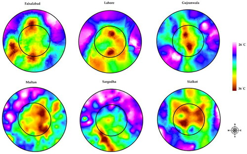
To measure the surface urban heat phenomenon and show the ecological conditions, UTFVI was calculated. For six major cities from 1992 to 2014, Figure 10 shows the spatial variation of urban heat field variance. The central buffer reflected the urban area with low vegetation cover while elevated built-up cover. Concentrated urban development has contributed to the destruction of the natural ecosystem in urban areas. UTFVI was divided by six separate ecological indices into six levels. The threshold values of the six levels are shown in Table 7. UTFVI data showed that due to the dispersion of urbanization flux out of it, the thermal field gradient was spreading out from the urban buffer. As a result, the urban thermal field gradient was drawn out of the urban buffer. The urban thermal field varied in the same direction of urban extent. The result showed that the highest UTFVI value (0.1608) was found in the city of Gujranwala, while the lowest value (0.0995) was found in the city of Faisalabad. The ecological situation of Gujranwala city was worse with the UTFVI max value of 0.16080 and excellent with the UTFVI min value of −0.16476 in some parts of rural areas. The UTFVI max value and spatial pattern showed that the strongest UHI was the urban area. We found that a greater portion of Gujranwala city had a very poor living condition and a similar spatial pattern to LST, based on UTFVI research. The UTFVI value was higher in center of buffer due to built-up sector.

Figure 10. Spatial visualization of UTFVI.

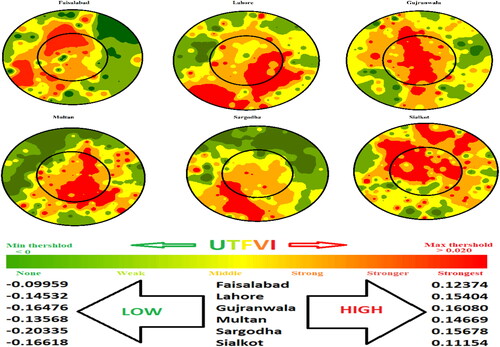
Table 7. Threshold values UTFVI (Liu and Zhang 2011).

Urban heat island phenomenon	Urban thermal field variance index
None	<0
Weak	0.000–0.005
Middle	0.005–0.010
Strong	0.015–0.015
Stronger	0.015–0.020
Strongest	>0.020

4. Statistical analysis

We examined the potential relationship between LST and LULC drivers (NDVI, and NDBI) to explore influencing factors. Vegetation covered area (NDVI) has a negative correlation with LST, while built-up areas (NDBI) displayed a strong positive correlation with LST on the basis that built-up areas were taken as urbanized according to the results of the classification. The relation between the indicators for land use (NDVI, NDBI) and LST as defined in Sections 4.1 and 4.2.

4.1. Relationship between LST and NDVI

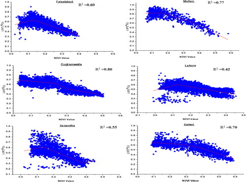
There was an important correlation between NDVI and LST, and a negative association between NDVI (high vegetation) and LST was observed. The increase in the magnitude of LST, as indicated, along with the decrease in NDVI values. NDVI and LST had a strong relationship when the correlation was made between NDVI and LST (Bokaie et al. 2016). In addition, a negative correlation was identified between LST and NDVI values on the basis of literature data during the study period (Kaplan et al. 2018). During 1992-2014, the average LST values were strongly and negatively correlated in all cities with NDVI. The decrease in NDVI values corresponded to an increase in buffer LST values. The determination coefficient (R²) values, as shown in Figure 11, were 0.60, 0.42, 0.80, 0.77, 0.55 and 0.70 in Faisalabad, Lahore, Gujranwala, Multan, Sargodha, and Sialkot, respectively. ANOVA's one-way statistical test concluded that there is a strong association between NDVI and LST in six cities with a significant = 0.01. With vegetation cover, NDVI values increased and, subsequently, LST values declined accordingly. The average NDVI value ranged between 0.1 (in the urban buffer) and 0.6 (in the rural buffer). Because of low vegetation, the urban buffer had the lowest NDVI concentration in all cities. With the growth of vegetation cover, NDVI values increased as the LST value results decreased. It was deduced in the rural buffer for 1992 and 1999 that the LST magnitude was reduced as a result of the increased NDVI value. It is shown that LST began to increase from rural buffer to urban buffer due to a decrease in NDVI and vegetated area values.

Figure 11. Piecewise regression between average NDVI and LST (1992-2014).(Extracted 3000 pixels’s value for each city to draw it).

4.2. Relationship between LST and NDBI

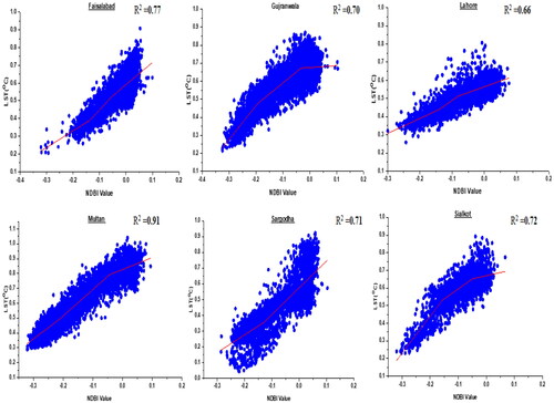
NDBI is also an important indicator of LULC changes and the results showed that in response to LULC changes, NDBI reflected the changes in the thermal climate. Due to extreme heat emitted from the heavily populated areas, urbanization has made the local climate warmer. (Houghton 2001). Higher NDBI values are interpreted by the densely built-up regions and the maximum temperature in the urban buffer was shown. A strong positive correlation was determined between the values of LST and NDBI with withal (Jamei et al. 2019). Using the piecewise regression model, the intensity of the relation between NDBI and LST in all the cities was calculated. In Faisalabad, Lahore, Gujranwala, Multan, Sargodha, and Sialkot, the coefficient of determination (R²) values were 0.77, 0.66, 0.70, 0.91, 0.71 and 0.72. The positive correlation indicated that in the urban buffer, the built-up area increased LST and was the main contributor to the impact of the an UHI. Figure 12 clearly shows that LST was increasing with the NDBI values from rural towards urban regions. The rural buffer had lower NDBI values (< 0), while the urban area had high NDBI values (> 0.01). The principal cause of higher temperatures was a higher NDBI value in the urban buffer. Urban temperatures have been stimulated by other factors, such as emissions, energy consumption, transport, and air conditioners. In six cities, the correlation between NDBI and LST was important at < = 0.01. Building materials had a high specific heat capacity in urban areas to absorb thermal radiation produced by the sun or by anthropogenic sources, and they absorbed radiation from the surrounding atmosphere during the night before it became thermal equilibrium. In keeping the cities warmer, particularly building heights, street canyons, road width, and construction material, the urban canopy also played a very vital role.

Figure 12. Piecewise regression between average NDBI and normalized LST (1992–2014). (Extracted 3000 pixels’ value for each city to draw it).

5. Discussion

In highlighting LST, the LULC changes review highlighted the strict relationship between LST and the management of land use. In particular, the present study highlighted the most notable LULC changes in terms of contribution to UTE. Urban coverage increased primarily in all cities during the study period and, secondly, other areas (barren land, rocky land, and sandy land) also increased. In contrast to the rural buffer, the urban buffer had higher LST values. The built-up area was particularly occupied by vegetated and water areas in the urban buffer. The geophysical processes that produced higher LST in the urban buffer were altered. It was also identified that higher LST trends were gradually heading to rural areas. Another main finding in the current study was that in most towns, the rate of incremental increase in the mean LST within the rural buffer was greater than urban. In the rural buffer, average improvements in LST values over the eight years were increased by 1.85 °C, 0.57 °C, 0.83 °C, 2.57 °C, 2.61 °C, and 0.68 °C respectively in Faisalabad, Gujranwala, Lahore, Multan, Sargodha and Sialkot. With the relationship between LULC and LST being studied, it was noted that urban areas had the highest LST(Simwanda et al. 2019). In addition, the LST average gradient decreased from the urban to the rural buffer, and its distribution was closely similar to the urban expansion trend (Rizwan et al. 2008, Li et al. 2018). The mean LST increased steadily from 1992-2014, beyond the spatial scale of the urban buffer in each city. These findings may be due to populated and impermeable surfaces being urban buffers. Similar results have been found that urban areas have the highest LST relative to other regions, water areas, and areas of vegetation (Ibrahim and Rasul 2017, Tran et al. 2017).

For example, Arshad et al. (2019) emphasised that LULC changes particularly urbanisation, have increased the mean temperature in Faisalabad in the past few years. The present study results are consistent with previous studies (Arshad et al. 2019), and Sajjad et al. (2015) concluded that the temperature of Lahore was particularly lower (Sajjad et al. 2015). Chung et al. (2004) clarified that urban expansion was a key contributor to the temperature rise in South Korean urban areas(Chung et al. 2004). In 2007, in Beijing, China, Liu et al. concluded that urban growth was increasing the mean temperature. The mean LST of built-up was greater than the vegetated cover and also the land cover function that contributed most to the LST is built-up (Liu et al. 2007). Lu et al. (2015) used Landsat images to assess the urban expansion of Shenyang city and its effect on the UTE (Lu et al. 2015).

The variance in temperature in urban and rural buffers help to understand the impact of SUHII on the study sites. Within the urban buffer, the SUHII phenomenon is very intense (Simwanda et al. 2019). Because of growing LST in the rural buffer and SUHII effect moved towards rural buffering. Our main results are consistent with previous research work peng et al. (2017) resulted in growing UHI effects outside the urban core, continuing urban growth and spending away from the urban centre (Fu and Weng 2018). In a very dense area, urbanisation and densification have caused heat to trap and increased SUHII. Vegetated areas have the ability to reduce and maintain the thermal intensity of densified urban areas, which is critical for sustainable urban planning (Pramanik and Punia 2020). The thermal physics of the built-up cover was also explained to SUHII by keeping in mind the thermal conductivity of the material, the basic heat power of the material, and thermal conduction, etc. (Chapin et al. 2005). The LULC modifications in the rural buffer could clarify this. The SUHII pattern was positive initially and negative after 2007, as rural LST continues to increase continuously (Figure 9). Based on the HECI study, built-up land positively contributed to a rise in LST in all cities during 1992-2014, while water bodies negatively contributed. In other cities, these findings are consistent with the previous report (Shi et al. 2015, Huang, Huang et al. 2019). The UTFVI value is greater in the urban than rural buffer. The thermal field intensity gradient was also moving toward rural buffers. The SUHII phenomenon faced all urban buffers and had the worst ecological conditions. Previous studies have shown similar UTFVI findings in different areas of the study (Liu and Zhang 2011, Renard et al. 2019).

The interactions and effects of NDBI and NDVI with LST have commonly been assessed in complex and temporal ways (Tran et al. 2006, He et al. 2010, Zhang et al. 2013). Mean LST in Suzhou City, China, showed a negative association with green space coverage.(Wu and Zhang 2018). These are also important LULC indicators and changes in NDVI/NDBI in response to LULC changes can indicate changes in the thermal climate. Thus, variability in thermal changes is observed by the study of NDVI changes. By generating a cooling effect in dense urban areas, vegetation plays a key role in sustaining eco-environmental sustainability (Weng et al. 2004, Amiri et al. 2009, Gunawardena et al. 2017). We concluded in the present study that an increase in LST was observed along with a decrease in NDVI values. There is a link between NDVI and LST that is substantial and negative. Based on the previous history of literature, a negative association was investigated between both LST and NDVI parameters (Zareie et al. 2016, Zareie et al. 2016, Kaplan et al. 2018, (Bokaie et al. 2016)). LST showed a declining trend in vegetated cover and the negative relationship between LST and NDVI was shown by several previous studies (Liu and Zhang 2011, Li et al. 2014, Shi et al. 2015). A study by (Saleem, Ahmad, and Javed 2020) studied the impact assessment of urban development on LST in major cities of Pakistan and resulted certain findings 1) NDVI showed negative relationship with the LST in Faisalabad city, 2) LST had showed the positive relationship with built-up in Multan city, and 3) a negative correlation observed between vegetation and LST in Lahore city, Pakistan. Land transformation associated impacts on LST and vegetated area resulted into decrease in LST in the Lahore, Pakistan (Mumtaz et al. 2020) Similarly, a strong negative association between LST and vegetation in Africa has been identified, which may support current study findings (Simwanda et al. 2019). In our findings the break points showed the detailed information of relation between NDVI and LST due to heterogeneity in the pixel values. Through beak points concluded that how changes in NDVI is relating with the LST. The piecewise linear regression was applied to check the detailed behavior of NDVI and LST shown in Figure 11. In addition, Jamei et al. (2019) also found a non-linear association in Melbourne between NDVI and LST and showed that elevated LST was observed with less vegetation in the region of the city (Jamei et al. 2019). In addition, Xie et al. (2013) found that the LST had a negative correlation between vegetation fraction coefficient (NDVI) and Liu and Zhang (2011) investigated the negative coefficient correlation between NDVI and LST (Liu and Zhang 2011, Xie et al. 2013). However, LST has a strongly positive correlation in the present study and a growing trend with NDBI in all major cities and scatter plots were made by extracting the pixel’s value across the urban and rural buffers. In Figure 12 piece wise linear regression showed detailed information of relation between NDBI and LST pattern through break points. The NDBI pixel values are varying and it showed its relation in detail with LST values. The results of the previous research are consistent with the findings of the current study. A study conducted by (Sadiq Khan et al. 2020) resulted that impervious surfaces positively contributed to increase the LST. The built-up area resulted into increased LST in the Lahore, Pakistan (Mumtaz et al. 2020). A study by (Saleem, Ahmad, and Javed 2020) resulted certain findings 1) positive correlation observed between NDBI (built-up) and LST in Faisalabad city, 2) LST had showed the positive relationship with built-up in Multan city, and 3) a positive correlation was found between built-up and LST in Lahore city, Pakistan. Jamei et al. (2019) noted that rises in the built-up region led to elevate LST and show a positive coefficient association between NDBI and LST(Jamei et al. 2019). Both of these factors contributed to slow wind velocity, resulting in no heat-wave exchange in urban areas. (Cui and Shi 2012). The positive association between LST and NDBI was shown by Tan et al. (2020) and Nimish et al. (2020), demonstrating the high impact of impermeable surfaces on urban temperatures (Nimish et al. 2020, Tan et al. 2020). In relation to LULC, Liu et al. (2020) evaluated the LST variation and concluded that the LST variation was associated positively with impermeable surfaces and negatively with vegetation (Liu et al. 2020). Urbanization reduces the capacity to store carbon and results in additional stagnant carbon dioxide in the environment that plays a crucial role in warming the earth's planet (Baumert and Pershing 2004). The 90 percent of anthropogenic carbon produced by burning fuels in major cities; sources of transport; and so on. Clearing land for cities, pavement surfaces, and highways are the key drivers of land-use transition, such as deforestation, which has limited carbon storage capacity (Svirejeva-Hopkins et al. 2004). Our current findings have shown that all cities and related problems are presented to UHI. New developmental schemes and housing societies have replaced the green patches in all towns. According to current findings, in order to reduce the swelling effect of the heat island, land planning studies carefully based on the natural capacity of the land to abandon its misuse and green spaces in the city are significant. The government should take urgent steps to push urban area tree plantations as it can reduce the amount of heat and increase the cities' groundwater table and air quality. It is helpful for administrators to consider the effect of LULC improvements on the LST and to follow effective policies to govern it. This study can be helpful for the policies making and sustainable urban planning in Punjab, Pakistan.

The current study considered the LULC drivers (NDVI and NDBI) to simplify the study because they directly involved to alter UTE. This study first comprehensive attempted to examine the long-term perspective changes in LULC and their impacts on the thermal environment, and only primary results were obtained. There are certain factors including population, landscape, and socioeconomic resulted to exuberate the UTE. In order to examine their quantitative relationship with UTE, there is a still need to undertake future research by considering these parameters.

6. Conclusion

A comparative analysis of spatiotemporal changes in UTE for Pakistan's six major cities (Faisalabad, Lahore, Gujranwala, Multan, Sargodha, and Sialkot) was conducted using Landsat-5, 7, and 8 data to explore the relationships between the spatial patterns, configuration, and composition of LULC maps with LST. Vegetation land was enormously transformed into built-up land in all six cities, and it was constantly extended from urban to rural buffer. In the rural buffer, the average LST value rose at a higher rate compared to the urban buffer due to the steady expansion of urbanization towards the rural buffer. Due to a rise in rural temperature at a greater rate, the disparity between urban and rural temperatures increased and the SUHII trend turned negative. The HECI showed that the heat contribution of the various land cover inputs was strongly pronounced for urban cover.

A significant finding in the current study is that all urban buffers have poor ecological conditions altogether. Due to the high SUHII effect, bad ecological conditions can lead to negative effects primarily on human health, including heatstroke, nervous system failure, cardiac and gastrointestinal problems. Statistical analysis showed that with the built-up area, LST was boosted. Areas with high NDVI (vegetation) had a negative correlation with LST, while a high positive correlation with LST was seen in built-up areas (NDBI). Because of the alteration of the bio-geophysical processes induced by LULC shifts, LST increased gradually. Our findings showed that high-resolution Landsat product data provided a better understanding through remotely sensed LST of the study of LULC changes and their effects on the thermal environment at landscape and regional scales (cities). The LULC (NDVI and NDBI) indicators have an important relationship with LST and can be used to research the SUHII effect. In addition, to eliminate the severity of the thermal environment, vegetated regions may play a vital role. A clear understanding of the effects of land change on the spatiotemporal changes of the LST and its contributing factors was established in the present study results using LST data collected from Landsat products in Punjab, Pakistan.

Author contributions

Conceptualization, B.C.; Data curation, A.D., A.A, Y.H., V.T., S.M., L.G., S.S; Formal analysis, A.D., Y.T., V.T., A.A., Y.H.; Funding acquisition, B.C.; Investigation, A.D., Y.T., A.A. V.T., A.K., H. Z., W.F, S.S; Methodology, A.D., B.C.; Resources, B.C.; Supervision, B.C.; Validation, A.D.; Writing – original draft, A.D., B.C.; Writing – review & editing, B.C.

Acknowledgments

The First author wants to thank the United States Geological Survey (USGS) https://earthexplorer.usgs.gov/ for Landsat bands images from 1992 to 2014 and the Chinese Government Scholarship Council (CSC) to support for Ph.D. study.

Disclosure statement

No potential conflict of interest was reported by the authors.

Correction Statement

This article has been republished with minor changes. These changes do not impact the academic content of the article.

Additional information

Funding

This work was supported by National Key R&D Program of China [Grant # 2017YFC0503904, 2018YFA0606001, 2017YFA0604301 & 2017YFA0604302], the research grants [41771114 & 41271116] funded by the National Natural Science Foundation of China, and the research grant [O88RA901YA] funded by the State Key Laboratory of Resources and Environment Information System.

References

- Ahmed S. 2018. Assessment of urban heat islands and impact of climate change on socioeconomic over Suez Governorate using remote sensing and GIS techniques. Egypt J Remote Sens and Space Science. 21(1):15–25.
- Amiri R, Weng Q, Alimohammadi A, Alavipanah SK. 2009. Spatial–temporal dynamics of land surface temperature in relation to fractional vegetation cover and land use/cover in the Tabriz urban area, Iran. " Remote Sens Environ. 113(12):2606–2617.
- Arshad A, Zhang W, Zaman MA, Dilawar A, Sajid Z. 2019. Monitoring the impacts of spatio-temporal land-use changes on the regional climate of city Faisalabad, Pakistan. Ann Gis. 25(1):57–70.
- Asmala A. 2012. Analysis of maximum likelihood classification on multispectral data. Appl Math Sci. 6(129-132):6425–6436.
- Balaghi R, Tychon B, Eerens H, Jlibene M. 2008. Empirical regression models using NDVI, rainfall and temperature data for the early prediction of wheat grain yields in Morocco. Int J Appl Earth Obs Geoinf. 10(4):438–452.
- Baumert K, Pershing J. 2004. Climate data: insights and observations. Pew Center on Global Climate Change. USA.
- Bokaie M, Zarkesh MK, Arasteh PD, Hosseini A. 2016. Assessment of urban heat island based on the relationship between land surface temperature and land use/land cover in Tehran. Sustain Cities Soc. 23:94–104.
- Cai D, Fraedrich K, Guan Y, Guo S, Zhang C. 2017. Urbanization and the thermal environment of Chinese and US-American cities. Sci Total Environ. 589:200–211.
- Cai X, Sharma BR. 2010. Integrating remote sensing, census and weather data for an assessment of rice yield, water consumption and water productivity in the Indo-Gangetic river basin. Agric Water Manage. 97(2):309–316.
- Cao W, Huang L, Liu L, Zhai J, Wu D. 2019. Overestimating impacts of urbanization on regional temperatures in developing megacity: Beijing as an example. Adv Meteorol. 2019:1–15. "
- Chapin FS, Sturm M, Serreze MC, McFadden JP, Key JR, Lloyd AH, McGuire AD, Rupp TS, Lynch AH, Schimel JP, et al. 2005. Role of land-surface changes in Arctic summer warming. Science. 310(5748):657–660.
- Chen X-L, Zhao H-M, Li P-X, Yin Z-Y. 2006. Remote sensing image-based analysis of the relationship between urban heat island and land use/cover changes. Remote Sens Environ. 104(2):133–146.
- Chung U, Choi J, Yun JI. 2004. Urbanization effect on the observed change in mean monthly temperatures between 1951–1980 and 1971–2000 in Korea. Clim Change. 66(1/2):127–136.
- Cui L, Shi J. 2012. Urbanization and its environmental effects in Shanghai, China. Urban Clim. 2:1–15.
- Dai Z, Guldmann J-M, Hu Y. 2018. Spatial regression models of park and land-use impacts on the urban heat island in central Beijing. Sci Total Environ. 626:1136–1147.
- Dempewolf J, Adusei B, Becker-Reshef I, Hansen M, Potapov P, Khan A, Barker B. 2014. Wheat yield forecasting for Punjab Province from vegetation index time series and historic crop statistics. " Remote Sensing. 6(10):9653–9675.
- Department of Economics and Social Affairs, U. N. 2019. U.N. World Population Prospects.
- Fan H, Yu Z, Yang G, Liu TY, Liu TY, Hung CH, Vejre H. 2019. How to cool hot-humid (Asian) cities with urban trees? An optimal landscape size perspective. Agric Meteorol. 265:338–348.
- Fu P, Weng Q. 2018. Responses of urban heat island in Atlanta to different land-use scenarios. Theor Appl Climatol. 133(1/2):123–135.
- Goovaerts P. 1997. Geostatistics for natural resources evaluation, Oxford University Press on Demand, Michigan, USA.
- Gorelick N, Hancher M, Dixon M, Ilyushchenko S, Thau D, Moore R. 2017. Google Earth engine: planetary-scale geospatial analysis for everyone. Remote Sens Environ. 202:18–27.
- Guha S, Govil H, Dey A, Gill N. 2018. Analytical study of land surface temperature with NDVI and NDBI using Landsat 8 OLI and TIRS data in Florence and Naples city, Italy. Eur J Remote Sens. 51(1):667–678.
- Gunawardena K, Wells M, Kershaw T. 2017. Utilising green and bluespace to mitigate urban heat island intensity. Sci Total Environ. 584-585:1040–1055.
- He C, Shi P, Xie D, Zhao Y. 2010. Improving the normalized difference built-up index to map urban built-up areas using a semiautomatic segmentation approach. Remote Sens Lett. 1(4):213–221.
- He B-J, Zhao Z-Q, Shen L-D, Wang H-B, Li L-G. 2019. An approach to examining performances of cool/hot sources in mitigating/enhancing land surface temperature under different temperature backgrounds based on landsat 8 image. Sustain Cities Soc. 44:416–427.
- Houghton. 2001. Climate Change 2001. The scientific basis. New York: Cambridge University Press.
- Huang Q, Huang J, Yang X, Fang C, Liang Y. 2019. Quantifying the seasonal contribution of coupling urban land use types on Urban Heat Island using Land Contribution Index: a case study in Wuhan, China. Sustain Cities Soc. 44:666–675.
- Ibrahim F, Rasul G. 2017. Urban land use land cover changes and their effect on land surface temperature: Case study using Dohuk City in the Kurdistan Region of Iraq. Climate. 5(1):13.
- Jain M, Dimri A, Niyogi D. 2017. Land-air interactions over urban-rural transects using satellite observations: analysis over Delhi, India from 1991–2016. Remote Sens. 9(12):1283.
- Jamei Y, Rajagopalan P, Sun QC. 2019. Spatial structure of surface urban heat island and its relationship with vegetation and built-up areas in Melbourne, Australia. Sci Total Environ. 659:1335–1351.
- Jones P, Lister D, Li Q. 2008. Urbanization effects in large‐scale temperature records, with an emphasis on China. J Geophys Res. 113(D16122)
- Kaplan G, Avdan U, Avdan ZY. 2018. Urban heat island analysis using the landsat 8 satellite data: a case study in Skopje, Macedonia. Multidiscip Digital Publis Instit Proc. 2(7):358.
- Karakus CB, Kavak KS, Cerit O. 2014. Determination of variations in land cover and land use by remote sensing and geographic information systems around the city of Sivas (Turkey). Fresenius Environ Bull. 23(3):667–677.
- Karakuş CB. 2019. The impact of land use/land cover (LULC) changes on land surface temperature in sivas city center and its surroundings and assessment of urban heat island. Asia-Pacific J Atmos Sci. 55(4):669–616.
- Kumar D, Shekhar S. 2015. Statistical analysis of land surface temperature-vegetation indexes relationship through thermal remote sensing. Ecotoxicol Environ Saf. 121:39–44.
- Landsat N. 2016. Landsat Project Science Office.
- Landsat. 2019. Science data users handbook. U.S Geological Survey (USGS) Landsat Project Science Office, Sioux Falls, USA.
- Li W, Bai Y, Chen Q, He K, Ji X, Han C. 2014. Discrepant impacts of land use and land cover on urban heat islands: A case study of Shanghai, China. Ecol Indic. 47:171–178.
- Lim H, Jafri M, Abdullah K, Alsultan S. 2012. Application of a simple mono window land surface temperature algorithm from Landsat ETM over Al Qassim, Saudi Arabia. Sains Malaysiana. 41(7):841–846.
- Li Y-B, Shi T, Yang Y-J, Wu B-W, Wang L-B, Shi C-E, Guo J-X, Ji C-L, Wen H-Y. 2015. Satellite-based investigation and evaluation of the observational environment of meteorological stations in Anhui province, China. Pure Appl Geophys. 172(6):1735–1749.
- Li J, Song C, Cao L, Zhu F, Meng X, Wu J. 2011. Impacts of landscape structure on surface urban heat islands: A case study of Shanghai, China. Remote Sens Environ. 115(12):3249–3263.
- Liu W, Ji C, Zhong J, Jiang X, Zheng Z. 2007. Temporal characteristics of the Beijing urban heat island. Theor Appl Climatol. 87(1-4):213–221.
- Liu K, Su H, Li X, Wang W, Yang L, Liang H. 2016. Quantifying spatial–temporal pattern of urban heat island in Beijing: An improved assessment using land surface temperature (LST) time series observations from LANDSAT, MODIS, and Chinese new satellite GaoFen-1. IEEE J Sel Top Appl Earth Observations Remote Sensing. 9(5):2028–2042.
- Liu L, Zhang Y. 2011. Urban heat island analysis using the Landsat TM data and ASTER data: A case study in Hong Kong. Remote Sens. 3(7):1535–1552.
- Liu F, Zhang X, Murayama Y, Morimoto T. 2020. Impacts of land cover/use on the urban thermal environment: a comparative study of 10 megacities in China. Remote Sens. 12(2):307.
- Li Y-y, Zhang H, Kainz W. 2012. Monitoring patterns of urban heat islands of the fast-growing Shanghai metropolis, China: using time-series of Landsat TM/ETM + data. Int J Appl Earth Obs Geoinf. 19:127–138.
- Li H, Zhou Y, Li X, Meng L, Wang X, Wu S, Sodoudi S. 2018. A new method to quantify surface urban heat island intensity. Sci Total Environ. 624:262–272.
- Li X, Zhou W, Ouyang Z, Xu W, Zheng H. 2012. Spatial pattern of greenspace affects land surface temperature: evidence from the heavily urbanized Beijing metropolitan area, China. Landscape Ecol. 27(6):887–898.
- Lu D, Song K, Zang S, Jia M, Du J, Ren C. 2015. The effect of urban expansion on urban surface temperature in Shenyang, China: an analysis with landsat imagery. Environ Model Assess. 20(3):197–210.
- Matthew MW, Adler-Golden SM, Berk A, Richtsmeier SC, Levine RY, Bernstein LS, Acharya PK, Anderson GP, Felde GW, Hoke ML. 2000. Status of atmospheric correction using a MODTRAN4-based algorithm. Algorithms for multispectral, hyperspectral, and ultraspectral imagery VI, International Society for Optics and Photonics.
- Mumtaz, Faisal, Yu Tao, Gerrit de Leeuw, Limin Zhao, Cheng Fan, Abdelrazek Elnashar, Barjeece Bashir, Gengke Wang, LingLing Li, and Shahid Naeem. 2020. ‘Modeling Spatio-Temporal Land Transformation and Its Associated Impacts on land Surface Temperature (LST)’, Remote Sensing, 12: 2987.
- Nichol JE. 1994. A GIS-based approach to microclimate monitoring in Singapore's high-rise housing estates. Photogramm Eng Remote Sens. 60(10):1225–1232.
- Nimish G, Bharath H, Lalitha A. 2020. Exploring temperature indices by deriving relationship between land surface temperature and urban landscape. Remote Sens Appl: Soc Environ. 18:100299.
- Pan J. 2016. Area delineation and spatial-temporal dynamics of urban heat island in Lanzhou City, China using remote sensing imagery. J Indian Soc Remote Sens. 44(1):111–127.
- Peng J, Jia J, Liu Y, Li H, Wu J. 2018. Seasonal contrast of the dominant factors for spatial distribution of land surface temperature in urban areas. Remote Sens Environ. 215:255–267.
- Pramanik S, Punia M. 2020. Land use/land cover change and surface urban heat island intensity: source–sink landscape-based study in Delhi, India. Environ Dev Sustain. 22(8):7331–7326. "
- Quintano C, Fernández-Manso A, Calvo L, Marcos E, Valbuena L. 2015. Land surface temperature as potential indicator of burn severity in forest Mediterranean ecosystems. Int J Appl Earth Obs Geoinf. 36:1–12.
- Raynolds MK, Comiso JC, Walker DA, Verbyla D. 2008. Relationship between satellite-derived land surface temperatures, arctic vegetation types, and NDVI. Remote Sens Environ. 112(4):1884–1894.
- Renard F, Alonso L, Fitts Y, Hadjiosif A, Comby J. 2019. Evaluation of the effect of urban redevelopment on surface urban heat islands. Remote Sens. 11(3):299.
- Rizwan AM, Dennis LY, Chunho L. 2008. A review on the generation, determination and mitigation of urban heat Island. J Environ Sci. 20(1):120–128.
- Sadiq Khan, Muhammad, Sami Ullah, Tao Sun, Arif UR Rehman, and Liding Chen. 2020. ‘Land-Use/Land-Cover Changes and Its Contribution to Urban Heat Island: A Case Study of Islamabad, Pakistan’, Sustainability, 12: 3861.
- Sahana M, Dutta S, Sajjad H. 2019. Assessing land transformation and its relation with land surface temperature in Mumbai city, India using geospatial techniques. Int J Urban Sci. 23(2):205–225.
- Sajjad SH, Batool R, Qadri ST, Shirazi SA, Shakrullah K. 2015. The long-term variability in minimum and maximum temperature trends and heat island of Lahore city, Pakistan. Sci Int. 27(2):1321–1325.
- Saleem, Muhammad Sajid, Sajid Rashid Ahmad, and Muhammad Asif Javed. 2020. ‘Impact assessment of urban development patterns on land surface temperature by using remote sensing techniques: a case study of Lahore, Faisalabad and Multan district’, Environmental Science and Pollution Research, 27: 39865–78.
- Santamouris M, Ban-Weiss G, Osmond P, Paolini R, Synnefa A, Cartalis C, Muscio A, Zinzi M, Morakinyo TE, Ng E, et al. 2018. Progress in urban greenery mitigation science–assessment methodologies advanced technologies and impact on cities. J Civil Eng Manage. 24(8):638–671.
- Sekertekin A, Kutoglu SH, Kaya S. 2016. Evaluation of spatio-temporal variability in land surface temperature: a case study of Zonguldak, Turkey. Environ Monit Assess. 188(1):30
- Shah B, Ghauri B. 2015. Mapping urban heat island effect in comparison with the land use, land cover of Lahore district. Pak J Meteorol. 11(22):37–48.
- Shalaby A, Tateishi R. 2007. Remote sensing and GIS for mapping and monitoring land cover and land-use changes in the Northwestern coastal zone of Egypt. Appl Geogr. 27(1):28–41.
- Shi T, Huang Y, Wang H, Shi C-E, Yang Y-J. 2015. Influence of urbanization on the thermal environment of meteorological station: satellite-observed evidence. Adv Clim Change Res. 6(1):7–15.
- Simwanda M, Ranagalage M, Estoque RC, Murayama Y. 2019. Spatial analysis of surface urban heat islands in four rapidly growing African cities. Remote Sens. 11(14):1645.
- Sobrino JA, Jiménez-Muñoz JC, Paolini L. 2004. Land surface temperature retrieval from LANDSAT TM 5. Remote Sens Environ. 90(4):434–440.
- Song X-P, Hansen MC, Stehman SV, Potapov PV, Tyukavina A, Vermote EF, Townshend JR. 2018. Author correction: global land change from 1982 to 2016. " Nature. 563(7732):E26–E26.
- Svirejeva-Hopkins A, Schellnhuber HJ, Pomaz VL. 2004. Urbanised territories as a specific component of the global carbon cycle. Ecol Modell. 173(2-3):295–312.
- Tan J, Yu D, Li Q, Tan X, Zhou W. 2020. Spatial relationship between land-use/land-cover change and land surface temperature in the Dongting Lake area, China. Sci Rep. 10(1):1–9.
- Tran DX, Pla F, Latorre-Carmona P, Myint SW, Caetano M, Kieu HV. 2017. Characterizing the relationship between land use land cover change and land surface temperature. ISPRS J Photogramm Remote Sens. 124:119–132.
- Tran H, Uchihama D, Ochi S, Yasuoka Y. 2006. Assessment with satellite data of the urban heat island effects in Asian mega cities. Int J Appl Earth Obs Geoinf. 8(1):34–48.
- Ullah S, Tahir AA, Akbar TA, Hassan QK, Dewan A, Khan AJ, Khan M. 2019. Remote sensing-based quantification of the relationships between land use land cover changes and surface temperature over the Lower Himalayan Region. Sustainability. 11(19):5492.
- Wang J, Huang B, Fu D, Atkinson PM, Zhang X. 2016. Response of urban heat island to future urban expansion over the Beijing–Tianjin–Hebei metropolitan area. Appl Geogr. 70:26–36.
- Weng Q, Lu D. 2008. A sub-pixel analysis of urbanization effect on land surface temperature and its interplay with impervious surface and vegetation coverage in Indianapolis, United States. Int J Appl Earth Obs Geoinf. 10(1):68–83.
- Weng Q, Lu D, Schubring J. 2004. Estimation of land surface temperature–vegetation abundance relationship for urban heat island studies. Remote Sens Environ. 89(4):467–483.
- Wu Z, Zhang Y. 2018. Spatial variation of urban thermal environment and its relation to green space patterns: Implication to sustainable landscape planning. Sustainability. 10(7):2249.
- Xie M, Wang Y, Chang Q, Fu M, Ye M. 2013. Assessment of landscape patterns affecting land surface temperature in different biophysical gradients in Shenzhen, China. Urban Ecosyst. 16(4):871–886.
- Yamamoto Y, Ishikawa H. 2020. Influence of urban spatial configuration and sea breeze on land surface temperature on summer clear-sky days. Urban Clim. 31:100578.
- Yang C, He X, Yan F, Yu L, Bu K, Yang J, Chang L, Zhang S. 2017. Mapping the influence of land use/land cover changes on the urban heat island effect—a case study of Changchun, China. Sustainability. 9(2):312.
- Yang J, Wang Y, August P. 2004. Estimation of land surface temperature using spatial interpolation and satellite-derived surface emissivity. J Env Inform. 4(1):40–44.
- Yuan F, Sawaya KE, Loeffelholz BC, Bauer ME. 2005. Land cover classification and change analysis of the Twin Cities (Minnesota) Metropolitan Area by multitemporal Landsat remote sensing. Remote Sens Environ. 98(2-3):317–328.
- Zareie S, Khosravi H, Nasiri A. 2016. Derivation of land surface temperature from Landsat Thematic Mapper (TM) sensor data and analyzing relation between land use changes and surface temperature. " Solid Earth. Discuss:1–15.
- Zareie S, Khosravi H, Nasiri A, Dastorani M. 2016. Using Landsat Thematic Mapper (TM) sensor to detect change in land surface temperature in relation to land use change in Yazd, Iran. Solid Earth. 7(6):1551–1564.
- Zhang Y, Balzter H, Liu B, Chen Y. 2017. Analyzing the impacts of urbanization and seasonal variation on land surface temperature based on subpixel fractional covers using Landsat images. IEEE J Sel Top Appl Earth Observ Remote Sens. 10(4):1344–1356.
- Zhang H, Qi Z-f, Ye X-y, Cai Y-b, Ma W-c, Chen M-n. 2013. Analysis of land use/land cover change, population shift, and their effects on spatiotemporal patterns of urban heat islands in metropolitan Shanghai, China. Appl Geogr. 44:121–133.
- Zhang K, Wang R, Shen C, Da L. 2010. Temporal and spatial characteristics of the urban heat island during rapid urbanization in Shanghai, China. Environ Monit Assess. 169(1-4):101–112.
- Zhou D, Bonafoni S, Zhang L, Wang R. 2018. Remote sensing of the urban heat island effect in a highly populated urban agglomeration area in East China. Sci Total Environ. 628/629:415–429.
- Zhou G, Wang H, Chen W, Zhang G, Luo Q, Jia B. 2020. Impacts of Urban land surface temperature on tract landscape pattern, physical and social variables. Int J Remote Sens. 41(2):683–703.
- Zhou D, Zhao S, Liu S, Zhang L, Zhu C. 2014. Surface urban heat island in China's 32 major cities: spatial patterns and drivers. Remote Sens Environ. 152:51–61.data a collection of facts from which conclusions may be drawn More (Definitions, Synonyms, Translation)