Multi-Regional landslide detection using combined unsupervised and supervised machine learning

Abstract

Landslide detection is concerned with delineating the extent of landslides. Most of existing works on landslide detection have limited geographical extents. Therefore, the models developed out of these studies might perform poorly when applied to regions with different characteristics. This study investigates an Object-Based Image Analysis methodology built on unsupervised and supervised Machine Learning to detect the location of landslides occurred in multiple regions across the world. The utilized data includes Sentinel-2 multi-spectral satellite imagery and ALOS Digital Elevation Model. In the segmentation stage, pre and post-landslide images undergo segmentation using K-means clustering. Following the segmentation stage and dataset preparation and removing highly-correlated features from the dataset, two Random Forest classifiers (RF1 and RF2) are trained and tested on two different datasets to measure the generalization level of the algorithms with RF1 dataset spanning over more geographical diversities than RF2 dataset. The results show that the RF models can successfully detect landslide segments with test precision = 0.96 and recall = 0.96 for RF1 and test precision = 0.90 and recall = 0.87 for RF2. Further validation shows that, compared to RF2, RF1 results in less mislabelled non-landslide segments.

Keywords:

• Landslide
• change detection
• Machine Learning
• OBIA
• K-means
• Random Forest

1. Introduction

Landslides are one of the most destructive and recurrent natural hazards worldwide. They are induced by natural factors such as extreme rainfall and earthquakes and by human intervention, including construction and mining. Landslides can occur in a wide range of lithological as well as geomorphological settings from coastal regions and river valleys, to hilly areas. They can also be associated with different types of land cover, such as urban environment, forests, bare lands and grasslands. A reliable inventory of historical landslides is a key component of any landslide spatial prediction such as landslide susceptibility and hazard mapping (Dou et al. 2020; Merghadi et al. 2020). Generating such inventory requires an accurate estimation of the location and/or time of individual landslide events which is typically referred to as landslide detection, mapping or identification. Landslide detection is also an important part of early response activities following geological and meteorological events such as earthquake and landfalls in hilly and mountainous areas, which requires identification of areas that are affected by these natural hazards (Ma et al. 2020). Satellite remote sensing has proved its usefulness in generating landslide inventories (Martha et al. 2011), assisting traditional time-consuming mapping methods that mostly rely on field survey and visual interpretation of aerial photographs (Lu et al. 2011). The use of earth observation data for detecting landcover change (e.g., landslides) has continuously increased during the last two decades. The value of this data stands out for its global geographical coverage, high temporal frequency, low cost, and the broad selection of spatial and spectral features of optical sensors (Chen et al. 2012). Moreover, multi-temporal imagery for natural hazard assessments has become an alternative source to study areas with limited public geo-data. Public platforms such as Google Earth Engine, U.S Geological Survey (USGS) Earth Explorer, and European Space Agency (ESA) Copernicus provide free access to satellite-based datasets, which enables various types of spatio-temporal analyses on a global scale. Imagery collections from public missions of ESA (e.g., Sentinel-2) and NASA (e.g., Landsat 8) programs are among primary sources of medium-resolution spatial datasets for monitoring global land changes and provide continuous records of satellite-based observations.

Landslide detection from satellite imagery falls in the general domain of object detection and classification. Object detection requires finding patterns in the images that can be diagnosed as a distinct entity. Object detection methods in remote sensing, in general, include classical pixel-based approaches (Cheng et al. 2004; Danneels et al. 2007; Tsangaratos and Ilia 2014) and more advanced techniques such as the Object-Based Image Analysis (OBIA), which has proved its usefulness in many geospatial applications (Platt and Rapoza 2008; Blaschke 2010; Lu et al. 2011; Martha et al. 2011; 2012; Dou et al. 2015; Feizizadeh et al. 2017), especially with medium-to-high and very-high-resolution satellite imagery. OBIA generally consists of two phases: image segmentation and segment classification. In contrast to pixel-based approaches, OBIA allows the integration of landslides diagnostic features such as spectral, spatial, and contextual features in the segmentation phase (Martha et al. 2010) that better resemble visual interpretation of aerial photographs (Feizizadeh et al. 2017) and reduce the influence of the single-pixel reflectance (Blaschke 2013). Landslide detection using OBIA has been the subject of research studies in recent years. Martha et al. (2012) conducted an object-based analysis of multitemporal panchromatic images for the creation of historical landslide inventories. Blaschke et al. (2014) established a semi-automated OBIA methodology for locating landslides in north-western Iran. Hölbling et al. (2015) developed a semi-automatic OBIA approach for landslide detection in northern Taiwan based on high-resolution satellite data and a Digital Elevation Model (DEM). Feizizadeh et al. (2017) suggested an OBIA methodology for detecting landslide-induced changes using spatial and spectral features of multi-temporal satellite images and by applying fuzzy logic membership functionality.

Object classification in remote sensing is typically done through rule-based techniques based on feature thresholds (Baraldi et al. 2006; Martha et al. 2012). However, over the past two decades and driven by the increase of computational power and emerging technologies such as cloud computing, the use of data-driven methods such as Machine Learning (ML) in remote sensing and for object classification has significantly increased. In this regard, the most applied data-driven methods are Maximum Likelihood Classification (Strahler 1980; Rajan et al. 2008), K-Nearest Neighbour (Cover & Hart Cover and Hart 1967; Grabowski et al. 2003), Minimum Distance to Mean Classifier, and Parallelepiped Classifier (Khorram et al. 2016), as well as ensemble tree methods (e.g., Random Forest and Gradient Boosting) (Briem et al. 2002; Ham et al. 2005), Support Vector Machines (SVM) (Camps-Valls et al. 2006; Inglada 2007), and Artificial Neural Networks (ANN) (Del Frate et al. 2007; Jensen et al. 2009). Previous scientific works highlight that non-parametric techniques such as RF are more suitable for object-based image classification of remotely sensed images than parametric ones since they can handle different statistical distributions (Melgani and Bruzzone 2002; Mountrakis et al. 2011; Stumpf and Kerle 2011; Puissant et al. 2014; O'Connell et al. 2015). Recently, Deep Learning (DL) has been increasingly used in satellite image classification given their relative independence from feature engineering, which can be a daunting task. For instance, Maggiori et al. (2017) proposed a fully CNN for dense pixel-wise classification of satellite imagery to produce fine-grained classification maps. Prakash et al. (2020) applied a combined U-Net and Res-Net CNN architecture for landslide detection using high-resolution multispectral data. Although DL is a powerful method for landslide detection, the study conducted by Ghorbanzadeh et al. (2019) on comparison of results obtained from different CNN architecture with classic ML methods such as ANN, RF and SVM suggests that DL methods do not automatically outperform the conventional ML methods and the superiority of DL methods depends mainly on their design and architecture.

Previous works on OBIA and landslide detection made use of training data and feature thresholds that were region-specific and therefore performed poorly when applied to new areas where the method was not developed for. To this date, only a few works have combined OBIA and ML for landslide detection from remote sensing data, with the majority of these works using ML in the classification phase of OBIA. To our knowledge, there have been only two studies in the past years which used ML in the segmentation phase (Martha et al. 2011; Keyport et al. 2018), too. Stumpf and Kerle (2011) explored the applicability and performance of RF in OBIA framework for detecting landslides using very-high-resolution satellite imagery. Parker (2013) conducted an object-based segmentation and made a comparative analysis of the performance of RF and SVM for landslide detection using Worldview-2 imagery. Tavakkoli Piralilou et al. (2019) combined OBIA with ML methods for detecting landslides in Nepal based on topographic features and post-landslide high-resolution PlanetScope multi-spectral images. Moreover, the published studies are mostly conducted in local areas using high-resolution images, with relatively pure background objects, such as vegetation only (Li et al. 2016).

In this paper, we present a landslide detection method that uses Sentinel-2 and ALOS DEM data within the OBIA framework by using K-means clustering as an unsupervised learning method in the segmentation phase and RF classification as a supervised learning method in the classification phase. In contrast to the majority of previous research studies, the current study is based on publicly available medium-resolution satellite images from multiple regions across the world with various landscapes and geomorphological settings and with different types of landslides not tied to a specific triggering factor. It is hypothesized that this variety of training samples allows training a more generalized model to be used in regions for which the model was not trained for. The main goal of this study is to evaluate the performance of this ML-based OBIA framework for landslide detection as a practical method that does not require extensive pre-processing of input data. The data used in this paper and the OBIA methodology are adopted from Herrera Herrera (2019).

2. Machine Learning

2.1. K-Means clustering

K-means clustering is an unsupervised ML algorithm (Steinhaus 1956; MacQueen 1967) that aims to partition or cluster n data points into K clusters in which each data point belongs to the cluster with the nearest mean (cluster centroid). K-means clustering minimizes within-cluster variances (squared Euclidean distances) and tends to find clusters of comparable spatial extent.

The clustering process starts with a first group of K randomly selected centroids (K is a user-defined input here). These centroids are used as the starting points for the K target clusters. Then every data point is assigned to the nearest cluster depending on the Euclidean distance of the data point and the centroid. Once the first iteration is finished, the mean of every cluster is taken as the new centroid for that cluster. The data points are then reassigned to the new clusters based on their distance from the nearest new centroids. This process is repeated until the location of centroids do not change significantly or once the maximum number of iterations is achieved.

2.2. Random forest classification

The Random Forest (RF) method, introduced by Breiman (2001), is an ensemble method for supervised learning used for classification and regression. For classification purposes, the RF algorithm is based on an ensemble of Decision Trees (DT) such that each tree depends on the values of a random vector sampled independently for all trees in the forest. Figure 1 shows an example RF with three DTs.

Figure 1. An example Random Forest with three Decision Trees.

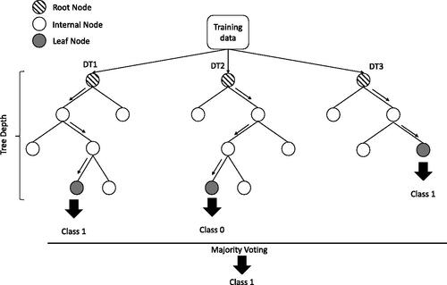
As shown in Figure 1, an RF is a set of DTs (3 in this example). Each DT is a set of internal nodes and leaves. In the internal node, a feature is randomly selected to make decision on how to divide the dataset into two separate sets with similar responses within (Class 0 or Class 1 here). The final features for internal nodes are selected with some criterion, which for classification tasks can be Gini impurity or information gain. One can measure how each feature decreases the impurity of the split. As such, the feature that results in the highest decrease is selected as the internal node. The process of splitting the dataset and the subsets into smaller sets is repeated on each derived subset at internal nodes in a recursive manner called recursive partitioning. The recursion is completed when the subset at a node (leaf node) has all the target class, or when splitting no longer adds value to the predictions (information gain) or when the maximum depth of the tree is reached. Once this procedure ends, the majority of the predicted classes at all DTs will be the final result of the trained RF.

2.3. Feature importance

In so-called black-box algorithms such as RF, it is difficult to understand how the algorithm comes up with the final solution. However, this does not mean that the algorithm and the resulting model is not interpretable. One way to interpret the model behaviour is to understand the relative importance of dataset features that the algorithm uses to learn the underlying pattern in the data. One type of feature importance is impurity-based feature importance known as Gini Importance or Mean Decrease in Impurity (MDI). MDI calculates the importance of every feature by computing how on average it decreases the impurity across all DTs.

2.4. Performance metrics

To measure the performance of a classifier algorithm, various metrics can be used. In this study we use well-known classification metrics namely accuracy, precision, recall and F1-score. The following equations show how these metrics are calculated: (1) $$\mathit{Accuracy}=\frac{TP+TN}{TP+TN+FP+FN}$$(1) (2) $$\text{Precision}=\frac{TP}{TP+FP}$$(2) (3) $$\text{Recall}=\frac{TP}{TP+FN}$$(3) (4) $$F1-\text{score}=2\cdot \frac{\text{Precision}\cdot \text{Recall}}{\text{Precision}+\text{Recall}}$$(4) where TP is true positive (a landslide correctly identified), TN is true negative (a non-landslide is correctly identified), FP is false positive (a non-landslide is incorrectly identified as a landslide), and FN is false negative (a landslide is incorrectly identified as a non-landslide).

3. Datasets

3.1. Optical satellite imagery

Sentinel-2 data is selected as the source for the input dataset as it provides publicly available optical satellite imagery data with the smallest Ground Sample Distance (GSD) of about 10 m. GSD is the distance between the centre of pixels measured on the ground, therefore a smaller GSD represents higher resolution of a digital image. Sentinel-2 has a global spatial coverage (56° S − 83° N) with multi-spectral images comprising of 13 spectral bands. The bands span the visible, Near-Infrared (NIR) and Short-Wave Infrared (SWIR) of the electromagnetic spectrum. Additional QA60 bands are included to support the detection and removal of clouds. For this research, we use Level-1C products (Sentinel-2 Multispectral Instrument Level-1C, TOA). They have radiometric and geometric corrections, including ortho-rectification and geo-referencing on a global reference system (WGS84) with sub-pixel accuracy.

3.2. Digital Elevation model

ALOS World 3 D-30m (AW3D30) is selected as the Digital Elevation Model (DEM) input, given its time span coverage (2006 to 2011 before the occurrence of the studied landslides in this research), global spatial coverage (between 60° S and 60° N latitudes) and availability. The dataset contains a horizontal GSD of approximately 30 m (about 1 arc-seconds latitude and longitude) generated from the 5 m resolution Digital Surface Model (DSM) (Tadono et al. 2014).

The slope or steepness of the ground surface is extracted from DEM. It is calculated using the 4-connected neighbours (horizontal and vertical neighbours of the central pixel) of each pixel.

3.3. Landslide database

To build and train the learning models in this study, a set of satellite images associated with landslide events is required. To identify landslide events, we reviewed online resources, social media, and the Global Landslide Catalog (GLC) of NASA Goddard Space Flight Center (Kirschbaum et al. 2010). From GLC, landslides larger than 10,000 m² (100 m × 100 m), with high location accuracy (<1,000 m) and with a date of occurrence after August 2015 (date of availability of Sentinel-2 data) are considered. We then use cloud-free pre- and post-event Sentinel-2 images through Google Earth Engine to build the landslide image collection (landslide database). The built landslide database consists of 29 entries that represent 29 satellite images distributed worldwide with a total of 185 landslide segments (Table 1).

Table 1. Landslide events used in this study.

ID	Event date	Longitude	Latitude	Landslide trigger	Country	# Landslide segments
L0	25-3-2017	−76.6625	1.168792	Downpour	Colombia	2
L1	27-6-2017	103.6529	32.06849	Continuous rain	China	28
L2	14-8-2017	−13.22985	8.43611	Unknown	Sierra Leone	3
L4	18-5-2016	80.431975	7.160808	Monsoon	Sri Lanka	5
L7	27-11-2016	101.613	3.366	Rain	Malaysia	1
L9	20-4-2017	−119.749	37.6786	Unknown	USA	1
L15	20-5-2017	−121.43238	35.865628	Rain	USA	13
L16	2-4-2017	−118.16398	47.88398	Downpour	USA	1
L17	18-1-2017	13.77821	42.42921	Earthquake	Italy	2
L18	3-7-2017	167.9676	−44.6861	Rain	New Zealand	2
L20	9-4-2017	111.82664	−7.723228	Downpour	Indonesia	1
L21	6-7-2017	130.93551	33.38917	Tropical cyclone	Japan	2
L22	6-7-2017	130.9002	33.38442	Tropical cyclone	Japan	6
L23	6-7-2017	130.76208	33.39482	Tropical cyclone	Japan	8
L25	6-7-2017	130.820741	33.403127	Tropical cyclone	Japan	1
L26	24-5-2017	130.811309	33.403094	Tropical cyclone	Japan	2
L27	24-5-2017	131.1126	33.4422	Tropical cyclone	Japan	4
L28	24-5-2017	131.089613	33.48504	Tropical cyclone	Japan	1
L40	11-4-2018	130.87977	33.52926	Unknown	Japan	6
L41	11-4-2018	130.896605	33.430754	Unknown	Japan	2
L43	6-9-2018	141.92972	42.71625	Earthquake	Japan	23
L47	6-9-2018	141.99075	42.716242	Earthquake	Japan	6
L48	6-9-2018	142.05179	42.71693	Earthquake	Japan	9
L55	15-11-2016	173.81687	−42.202247	Earthquake	New Zealand	15
L56	15-11-2016	173.81687	−42.157233	Earthquake	New Zealand	6
L57	15-11-2016	173.756415	−42.112203	Earthquake	New Zealand	2
L58	15-11-2016	173.877412	−42.202231	Earthquake	New Zealand	15
L59	15-11-2016	173.87741	−42.157217	Earthquake	New Zealand	17
L75	19-6-2018	85.890295	27.908346	Rain	Nepal	1

4. Methodology

4.1. General framework

The developed methodology consists of three key stages: image pre-processing, image segmentation (K-means), and segment classification and landslide detection (RF classification) (Figure 2).

Figure 2. Methodology Overview. (a) Pre-processing. (b) Image segmentation and feature extraction. (c) Segment classification and landslide detection (modified after Herrera Herrera 2019).

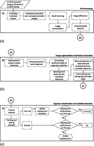
Next, the elements of the general framework are elaborated in detail.

4.2. Pre-processing

To retrieve cloud-free images before and after the occurrence of landslides, a pre-processing algorithm is developed based on the following three steps:

1. Find pre- and post-landslide event images with maximum cloudiness of 30% within four months before and after the date of the landslide event.

2. If no images with maximum cloudiness of 30% are found within this time frame, then find the first pre- and post-event images (with maximum cloudiness of 30%) within eight months before and after the landslide event.

3. If no image is found, apply the image composition technique. It consists of identifying the best pixels within a pre-defined temporal window. This temporal window is set to a maximum of one year.

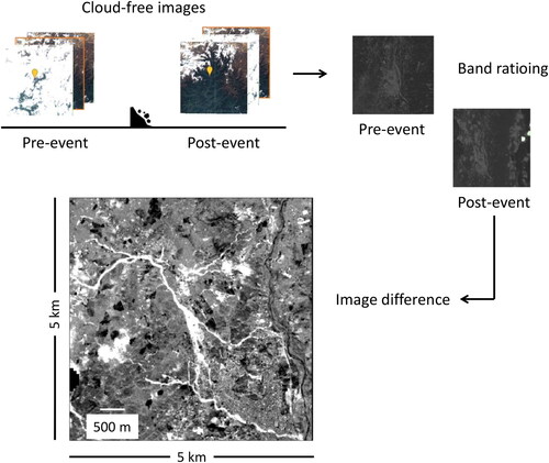
To find the most appropriate image, using Google Earth Engine, a large time-series of Sentinel-2 satellite imagery is analyzed based on the date and location of landslides. In the next step, the image difference of pre- and post-landslide images is obtained to minimize the misleading effect of landslides that occurred in the same area before the occurrence of the target landslide(s). Image differencing (Figure 3) stage requires band ratioing and normalization, to be elaborated later in this paper (see Section 4.2.2). After image differencing, the features per pixel of the output image are extracted and stored. The images are downloaded using a fixed bounding box of 5 km × 5 km. The size of 5 km × 5 km is selected to reduce the number of non-landslide segments in the subsequent analyses and to provide enough contextual features to distinguish landslides from the rest of the background segments. Moreover, this size allows efficient handling of the image acquisition from Google Earth Engine.

Figure 3. Image pre-processing stages (landslide L0, see Table 1 for details) (modified from Herrera Herrera 2019).

In the following sub-sections, the features extracted in the pre-processing stage are explained along with the methods used to calculate them.

4.2.1. Land cover indices

When a landslide occurs in a vegetated area, it removes or covers the surface vegetation along its travel path. A vegetated area shows high reflectance values in the Near-Infrared (NIR) bands, whereas a bare ground shows low NIR reflectance. This fact is used to define Normalized Difference Vegetation Index NDVI and Green Normalized Difference Vegetation Index GNDVI that can be used for landslide detection in vegetated areas: (5) $$\mathit{NDVI}\left(i,j\right)=\frac{\mathit{NIR}\left(i,j\right)-R\left(i,j\right)}{\mathit{NIR}\left(i,j\right)+R\left(i,j\right)}$$(5) (6) $$\mathit{GNDVI}\left(i,j\right)=\frac{\mathit{NIR}\left(i,j\right)-G\left(i,j\right)}{\mathit{NIR}\left(i,j\right)+G\left(i,j\right)}$$(6) where $(i,j)$ indicates the individual pixels in an n-pixel by m-pixel image, $(i,j):i=1,\dots ,n;j=1,\dots ,m.$

Additionally, the standard deviation NDVI_std of the NDVI image is made. This is done by applying a convolution that computes standard deviation of a 7 × 7 pixels kernel moving over the NDVI image.

Another land cover index is the Brightness Index (BR). Areas affected by landslides often have high BR values due to loss of vegetation and exposure of fresh rock and soil (Martha et al. 2010). Very high and very low values of BR relative to the landslides signature are used in this research to detect and remove clouds and shadows, respectively. The BR is calculated for pre- and post-event images based on Red, Green and Blue bands using the following equation: (7) $$BR=\frac{1}{R\left(i,j\right)+G\left(i,j\right)+B\left(i,j\right)}$$(7)

4.2.2. Image difference indices

An intuitive way to detect changes between two images taken at different times is by subtracting the grey values in the diverse bands of one image from those of the other image, pixel by pixel. However, when it comes to satellite images, brightness differences between pre-event and post-event images are not only caused by changes in terrain characteristics, but they are affected by inevitable changes in illumination conditions. Main causes of illumination changes are:

• Change in perspective resulting in differences in brightness in hilly terrain (slope and aspect)

• Different sunlight incident angle in time causing differences in shadowed areas and thus differences in brightness

• Seasonality causing changes to sunlight strength

• Different atmospheric conditions, including changes in the cloudiness level.

Given the possible changes to illumination conditions, the images have to be pre-processed prior to the image differencing. Two appropriate pre-processing methods are band ratioing and image normalisation. Band ratioing assumes that the differences in illumination affect nearby electromagnetic (EM) bands, similarly. It is usually computed by dividing the red band by the green band R(i,j)/G(i,j). Image normalizing reduces the effects of atmospheric differences, shadow and seasonal differences of sunlight strength. Normalization can be best explained using the following equation: (8) $$v_n^{t1}=\left(\frac{{\overline{v}}_{}^{t2}}{{\overline{v}}_{}^{t1}}\right)v_{}^{t1}$$(8) where $v_n^{t1}$ is the normalized value of band value $v_{}^{t1}$ of the pre-event image at time t₁, ${\overline{v}}_{}^{t1}$ is defined as the mean of the band values of the pre-event image, and ${\overline{v}}_{}^{t2}$ is defined as the mean of the band values of the post-event image at time t₂.

Upon band ratioing and normalization, three key landslide diagnostic features are calculated from the pre and post-event images:

4.2.2.1. Red-over-Green difference (RGD)

RGD is computed using the ratio of Red and Green bands from pre- and post-event images. (9) $$\mathit{RGD}\left(\mathrm{i},\mathrm{j}\right)={\frac{R\left(i,j\right)}{G\left(i,j\right)}|}_{t_2}-{\frac{R\left(i,j\right)}{G\left(i,j\right)}|}_{t_1}+c$$(9) where t₁ is the first date (pre-event), t₂ is the second date (post-event), and $c$(= 0.5 in this study) is a constant to produce positive values.

4.2.2.2. Vegetation index difference (VID)

VID is calculated using normalized NDVI values NDVI_n (i,j) from pre-event image and absolute NDVI values NDVI(i,j) from post-event image: (10) $$\mathit{VID}\left(i,j\right)=\mathit{NDV}{I}_n{\left(i,j\right)}_{t_1}-\mathit{NDVI}{\left(i,j\right)}_{t_2}$$(10)

4.2.2.3. Brightness difference (BRD)

The BRD is computed using normalized BR values BR_n (i,j) from pre-event image and absolute BR values BR(i,j) from post-event image as follows: (11) $$\mathit{BRD}\left(i,j\right)=B{R}_n{\left(i,j\right)}_{t_1}-BR{\left(i,j\right)}_{t_2}$$(11)

These features along with other topographic and spectral features will be later used to identify every pixel and the belonging segment.

4.3. Image segmentation and feature extraction

4.3.1. Segmentation

Image segmentation is the building block of OBIA (Lu et al. 2004) as the accuracy of the classification process is directly influenced by the segmentation quality (Lemmens 2011; Feizizadeh et al. 2017). Blaschke (2010) defines image segmentation as the subdivision of an image into spatially continuous, disjoint, and relatively homogeneous regions.

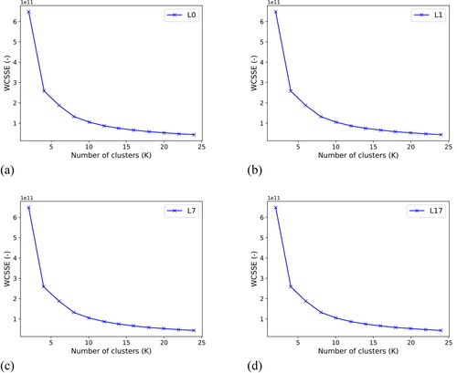
In this research, we use the operational large-scale segmentation algorithm proposed by Shepherd et al. (2019) for image segmentation based on RGD values (see (9)). This algorithm, which uses K-means clustering method, is a suitable approach for segmentation of satellite images due to its effectiveness and simplicity in parameter tuning across a large variety of scenes and its low-computational cost for large geographical areas. The key tuning parameters that condition the quality of the segmentation to preserve landslide candidate segments (avoiding landslide and non-landslide mixture) are the minimum number of pixels and the number of K-means clusters K. The minimum number of pixels is set to 80, a value slightly lower than the smallest size of the target landslides defined within the scope of this research (100 pixels). The optimal number of clusters for all images is estimated as K = 8 using the elbow method (Wikipedia 2020). The basic idea of this method is to fit the model with a range of values of K and minimize the Within-cluster Total Sum of Squared errors (WCSSE) over all clusters. Generally, the first clusters add most of the information, and at some value of K, the gain drops dramatically and gives a point of inflection on the plot (the elbow) that is considered as a good indicator of the optimal number of clusters (Bholowalia and Kumar 2014). In Figure 4, the reduction of WCSSE with the increase in the number clusters K is displayed for four of landslide images listed in Table 1. The elbow plots show comparable results for different landslide events, where the points of inflection or optimal numbers of clusters (x-axis) show approximately the same value (K = 8). The same behaviour was observed in other landslide images.

Figure 4. Elbow plots for the landslides L0, L1, L7, L17 (from Herrera Herrera 2019).

While a low value of K merges landslides with non-landslides segments, a higher value of K leads to over-segmentation but preserves landslides of different sizes. According to Shepherd et al. (2019), a certain degree of over-segmentation is generally accepted as merging strategies can be later applied to objects of the same cluster. In contrast, under-segmentation cannot be recovered during classification as target objects have been already misidentified or merged with larger segments (Debeir 2001) and consequently, spatial and contextual information will be lost. Therefore, we increase the selected K value and experimentally adjust it to reduce the chance of under-segmentation for the landslide segments. This results in K = 19 for segmentation in this study.

4.3.2. Grouping pixels of every segment

Once the segments are created, features of constituent pixels of a segment are grouped to produce features per segment. The feature statistics within segment polygons are calculated using RSGISLib (Shepherd et al. 2019) to generate attribute tables per image with rows representing the segments and columns representing the values of the features. As shown in Table 2, the mean feature values of pixels within every segment are mainly used as the representative values for the corresponding segments. This decision is made after several sensitivity analyses to estimate the best representing statistics for segments. For spatial features, the maximum slope and elevation as well as minimum elevation per segment are also calculated.

Table 2. Landslide diagnostic features at segment level.

Features	Feature type	Statistics per segment	Target Image	Source
B2, B3, B4, B8 bands	Spectral	mean	post-event	Sentinel-2
NDVI	Spectral	mean	post-event	Sentinel-2
GNDVI	Spectral	mean	post-event	Sentinel-2
Brightness	Spectral	mean	post-event	Sentinel-2
RGD	Spectral	mean	pre- and post-event	Sentinel-2
VID	Spectral	mean	pre- and post-event	Sentinel-2
BRD	Spectral	mean	pre- and post-event	Sentinel-2
NDVIstd	Contextual	mean	post-event	Sentinel-2
Slope	Spatial	mean, maximum	pre-event	AW3D30(2011)
Elevation	Spatial	mean, maximum, minimum	pre-event	AW3D30(2011)

4.3.3. Final dataset

Once diagnostic features are assigned to every segment, the next step is to create a landslide and non-landslide dataset from labelled segments (1 for landslide and 0 for non-landslide).

Selecting all segments for image classification will result in a highly imbalanced dataset which can skew the RF and most of other ML algorithms towards the majority class (non-landslides here). Moreover, for landslides of small size, it is not always feasible to identify and label correctly the landslide segments from medium-resolution satellite images, which will increase the chance of mislabelling and therefore inaccurate ML modelling later. To resolve these issues, we check every segmented image and manually label landslide and non-landslide segments for which we have high certainty in correct labelling. Also, we only provide labels for a fraction of segments to make sure that the landslide and non-landslide labelled segments are in good balance. In doing so, we ensure to select a variety of non-landslide segments (vegetated and non-vegetated) to obtain a generalizable ML model in the next stage.

4.4. Segment classification and landslide detection

Random Forest classification is used to classify landslides and non-landslide segments identified in the segmentation stage. The classification algorithm returns a binary output with landslides as the positive class (labelled as 1) and non-landslides as the negative class (labeled as 0). A subset (e.g., 80%) of the built sample dataset (see Section 4.3.3) is used to train the RF classifier model, while the rest (e.g., 20%) is used to test the trained model. To assess the extent to which every feature is discriminative, we use the Mean Decrease Impurity (MDI) implemented within the RF algorithm. When using MDI, RF computes the amount that each feature decreases the weighted impurity in an individual tree (Biau and Scornet 2016). With the Gini index or measure of the node impurity (quality of a split), the features are ranked after averaging the total decrease in the node impurity over all trees in the forest.

The RF hyper-parameters are tuned using cross-validation on the training dataset, divided into N equal sets, in order to find the model with best predictive performance. The optimal values are obtained by testing possible combinations using the GridSearchCV method available in Scikit-Learn Machine Learning python library (Scikit-Learn, 2020a). Given a grid of parameters, GridSearchCV builds a model on selected N-1 sets and evaluates the model built based on all parameter combinations on the N^th validation set. This process is repeated on all N sets one by one (training on N-1 sets and validating on N^th set) and the performance of the model is recorded. The parameter set that results in the highest performance during cross validation is selected as the final hyper-parameters.

5. Results

5.1. Segmentation

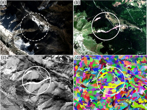
The applied segmentation strategy (see Section 4.3.1) allows to detect and isolate changes in pixels reflectance that are likely related to the occurrence of landslide events. As an example, Figure 5 shows a large-scale landslide occurring in a remote area in Italy. Although the large landslides are often mixed with vegetation, the applied segmentation on RGD image (Figure 5c) correctly delineates the borders of this large landslide as shown by light yellow segments in circled area of Figure 5d.

Figure 5. Image pre-processing and segmentation (from Herrera Herrera 2019); sample in a remote area in Italy (L17 in Table 1). (a) Cloud-free pre-landslide image. (b) Cloud-free post-landslide image. (c) Image difference using RGD. (d) Image segmentation.

Upon segmentation of images, we label landslide and non-landslide segments using the procedure explained in Section 4.3.3. This results in 185 landslide and 280 non-landslide segments (total of 465 segments) out of 29 images (see Table 1). The final dataset is then created using these labels and the diagnostic features presented in Table 2.

5.2. Classification

5.2.1. Feature analysis

It is important that the features used for building and training the RF model are not highly correlated. Highly correlated features in RF training can result in misleading results and interpretation of the model (e.g., in feature importance analysis). Figure 6 shows the map of Pearson Correlation Coefficient (PCC) of the segment features in this study (Table 2) based on the selected landslide and non-landslide segments.

Figure 6. Correlation map of features used in this study for the selected landslide and non-landslide segments.

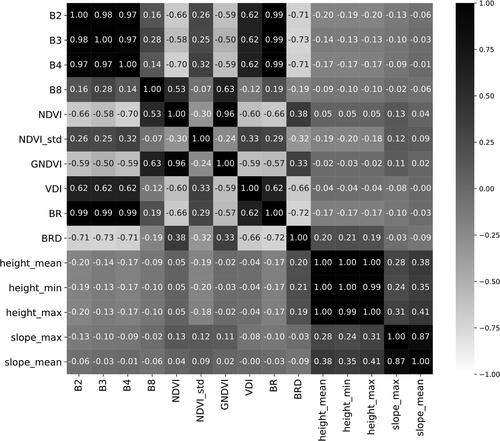
It is clear from Figure 6 that certain features are highly correlated. Setting PCC = ±0.85 as the threshold for high correlation, we then select the final features for model training. These features are: B8, NDVI, NDVI_std, VDI, BR, BRD, height_mean and slope_max.

5.2.2. Model training

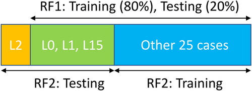
The input data for classification was organized using two different approaches. In approach 1, we first remove segments of case L2 (15 landslide and non-landslide segments) from the dataset and then randomly split the dataset into 80% train set and 20% test set. The RF model trained on this train set is called RF1. In approach 2, we set aside all labeled landslide and non-landslide segments associated with events L0, L1, L2 and L15 (see Table 1) as the test set (122 out of 456 segments ∼ 26% of all segments) and the remaining data is used for training the RF model. The resulting RF is called RF2. The reason for selecting those events in approach 2 is their geographical diversity (Colombia, China, Sierra Leone and USA), which can be useful in evaluating this study and its generalisation across multiple different regions across the globe. The selection of L2, as the unseen data for both RF1 and RF2, is an arbitrary choice. Since L2 segments are not used in training RF1 and RF2 models, they can be used later for a fair comparison of the two model. Figure 7 illustrates the train and test sets used for RF1 and RF2.

Figure 7. Train and test sets used for RF1 and RF2.

For both RF1 and RF2, we perform cross validation with 5 training and validation subsets (folds) on the associated train set. The candidate hyper-parameters as well as the final selections for RF1 and RF2 are shown in Table 3.

Table 3. RF candidate hyper-parameters in this study.

Hyper-parameter	Candidates	RF1	RF2
'bootstrap'	True	True	True
'max_depth'	10, 20, 50, 100, 500	10	10
'max_features'	2	2	2
'min_samples_leaf'	1, 2, 3, 4, 5	1	2
'min_samples_split'	2, 5, 10	5	10
'n_estimators'	10, 50, 100, 200, 500, 1000	50	10

As shown in Table 3, we use bootstrapping for RF classification, which means that RF internally uses random samples with replacement in training phase to yield a predictive model with hypothetically minimum variance. More details about the RF hyper-parameters can be found at Scikit-Learn library webpage (Scikit-Learn, 2020b).

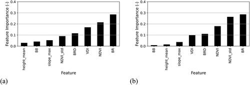
When using multiple features for classification, it is known that not all features may have similar contributions to the final model. Figure 8 clarifies the importance of the utilized features in RF training for both models RF1 and RF2.

Figure 8. Feature importance using the final model and the corresponding train dataset: (a) RF1, (b) RF2.

5.2.3. Model assessment

With all landslide diagnostic features resulted from correlation analysis and after cross-validation and training, we test the models on their associated test sets. Table 4 shows the performance metrics of the two models where LS is the total number of landslide segments and NLS is the total of non-landslide segments used in training and testing.

Table 4. Performance metrics of the trained and tested RF models.

Model	LS	NLS	TP	TN	FP	FN	Accuracy	Precision	Recall	F1-score
RF1 - train	147	213	145	213	0	2	0.99	0.99	1.00	1.00
RF1 - test	35	55	33	53	2	2	0.96	0.96	0.96	0.96
RF2 - train	135	208	135	204	4	0	0.99	0.98	1.00	0.99
RF2 - test	49	73	39	66	7	10	0.86	0.90	0.87	0.89

6. Discussion and further validation

6.1. Feature importance

Figure 8 shows the impurity-based feature importance for the final features used in training the RF models. It is evident that spectral and difference features display higher contribution to the final model than topography features by having BR, NDVI, NDVI_std, BRD and VDI as the 5 most important features. This is mainly due to selection of training data from the same scene that landslides took place (hilly/mountainous areas). Although topography features may not be that useful in distinguishing landslides and non-landslide segments in hilly areas, they are deemed to be useful for landslide detection where there is a sharp contrast in areas with flat and steep terrains. Single band B8 also does not show a significant contribution to the performance of the trained models. In both RF1 and RF2 models, post-landslide BR and NDVI are among the first three most important features. This means that the model uses the land cover main features after the occurrence of the landslide to detect landslides. However, such features can potentially result in mislabelling non-landslide segments as landslides for non-vegetated segments. This can be alleviated by using BRD and VDI as difference features that consider both pre- and post-landslide images.

6.2. Model performance

The results of model evaluation on train and test sets are shown in Table 4. Clearly, RF1 shows better performance than RF2 mainly because RF1 was trained on more diverse segments and areas and could learn more from different patterns existed in the associated dataset. Nonetheless, the performance of RF2 in the test set shows signs of generalisation on areas, that the model could not “see” during the training phase (in China, Sierra Leone, Colombia and USA). To further study the performance of the models, we apply the models on all segments of L0, L1, L2 and L15 landslides. It is noted that none of the models have seen L2 landslides. RF2 did not see L0, L1 and L15, either. Additionally, RF1 was trained on only a fraction of the segments of L0, L1 and L15. By colour coding the segments, we consider the ratio of the trees voting for landslide (LTR) to the total number of trees in the associated forest as a measure if a segment belongs to landslide or non-landslide segments. As a result, four classes are formed. The limits of LTR in each class is presented in Table 5.

Table 5. Segment classes in classification.

Class	LTR Limits	Description	Binary interpretation	Color code
1	0-0.33	Non-landslide	Non-landslide	green
2	0.33-0.50	Uncertain non-landslide	Non-landslide	yellow
3	0.50-0.67	Uncertain landslide	Landslide	orange
4	0.67-1.00	Landslide	Landslide	red

The four classes are formed for better interpretation and comparison of the classification results. For RF binary classification with two classes, LTR = 0.5 is the boundary between non-landslide (green and yellow) and landslide (orange and red) classes. Figures 9–12 show the overall results of the two models along with the pertained post-landslide Sentinel-2 images for the selected cases. The colour bar for all these figures is the same as that of Figure 9b.

Figure 9. Landslide detection for L0: (a) post-landslide optical image, (b) segmentation and final classification with RF1 model, (c) segmentation and final classification with RF2 model post-landslide image.

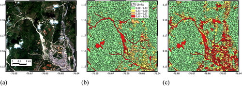
Figure 10. Landslide detection for L1: (a) post-landslide optical image, (b) segmentation and final classification with RF1 model, (c) segmentation and final classification with RF2 model post-landslide image.

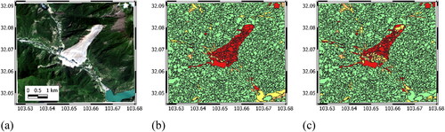
Figure 11. Landslide detection for L2: (a) post-landslide optical image, (b) segmentation and final classification with RF1 model, (c) segmentation and final classification with RF2 model post-landslide image.

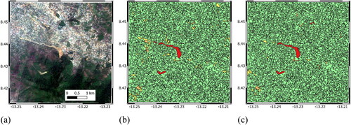
Figure 12. Landslide detection for L15 (center of the image): (a) post-landslide optical image, (b) segmentation and final classification with RF1 model, (c) segmentation and final classification with RF2 model post-landslide image.

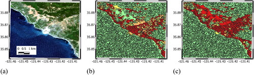
As shown in Figures 9–12, both RF1 and RF2 models show promising performance in identifying landslide segments. RF1 shows a better performance than RF2 in distinguishing non-landslide segments (classes 1 and 2) from landslide segments (classes 3 and 4). This is especially highlighted in identifying urban areas in L0 (Figure 9) and some non-vegetated segments in L15 (Figure 12). Fractions of L0 and L15 are part of the RF1 training, which can explain the difference between RF1 and RF2 performances on these two cases. It is clear from Figures 9 and 10 that both RF1 and RF2 mislabelled cloud segments as landslide (class 3 or 4). Similarly, for L15, the road segments along the coastline are classified as landslide by both RF1 and RF2. The fair comparison of the two models can be made on L2 in Sierra Leone (Figure 11), where both RF1 and RF2 successfully find main landslide segments and distinguish them from the downstream urban settlement. Overall, it seems the two model shows level of generalisation that can be useful in detecting landslide segments (true positive). The results show that correct labelling of non-landslide segments (true negative), is a more challenging tasks for the trained models. This is mainly due to similarity of non-landslide segments with low level of vegetation to landslide segments. The image difference and band ratioing may not provide further help here, which can be due to drastic change in illumination conditions between pre- and post-landslide images. Furthermore, given the time interval of up to 8 months between pre and post-landslide images, land cover features can undergo seasonal changes, which affects the corresponding spectral features in the Sentinel-2 data. A practical remedy here can be in the pre-processing stage by masking misleading objects such as roads and cloud patches before segmentation so that the segments are not “contaminated”. To that end, mislabelling roads can be avoided by using sources such as OpenStreetMap (https://www.openstreetmap.org/) for identification of unpaved roads, whereas mislabelling clouds can be avoided by quick visual inspection in the pre-processing stage.

7. Conclusions and future work

In this paper, we showed how publicly available data can be used to build and train ML-based landslide detection models to be used on multiple regions across the world. To achieve this, we collected 29 pre- and post-landslide scenes from Sentinel-2 images and used unsupervised learning (K-means) under the OBIA framework for segmentation of the images. The segment features were obtained from the basic statistics of the spectral bands (Sentinel-2 image) and terrain information (from the associated ALOS DEM) of the bounded pixels in every segment. Uncorrelated features were used as the final features: NDVI, NDVI_std, VDI, BR, BRD, height_mean and slope_max. We manually selected landslide and non-landslide segments and used the final dataset to train two RF models; RF1 and RF2, where RF1 was trained using more diverse data compared to RF2. The results showed that the RF models could successfully detect landslide segments with test precision = 0.96 and recall = 0.96 for RF1 and test precision = 0.90 and recall = 0.87 for RF2. The two models were further evaluated on entire segments of selected landslide images. It was revealed that the number of false positive (mislabelled non-landslide segments) in RF1 was lower than RF2 (implied also from the recall value), since RF1 was trained on more cases and could learn more diverse patterns in the training set.

Although we achieved promising results in this study, more landslide and non-landslide segments are needed in order to increase the performance and reliability of the landslide detection model. This can be regarded as the major limitation of our study, which can be alleviated in future by adding more data to the landslide database that we created. Another limitation that we see in our approach and similar works is using multi-spectral data as the main data source for landslide detection. Two major drawbacks are observed in this regard:

1. It is not always possible to position timely post-landslide imagery (within few hours to few days) given that most landslides are triggered by rainfall and therefore cloud contamination of immediate post-landslide images can be inevitable. Using cloud removal algorithms may not help either, because the landslide segments can be missed using those algorithms. A remedy for this limitation can be microwave remote sensing data (e.g. Sentinel-1) which is far less affected by atmospheric conditions compared to multi-spectral data.

2. Using multi-spectral data, it is likely that non-vegetated segments are classified as landslide segments which increase the number of false positives. This can be corrected by manual intervention, but it can be a cumbersome task especially if there are many false positives. Here, microwave remote sensing data and techniques such as Interferometric Synthetic Aperture Radar (InSAR) can be helpful for using change in elevation as another feature to detect landslides and distinguishing them from non-landslide segments.

The limitations and solutions discussed above are subject of our future studies.

Authors contribution

Faraz S. Tehrani & Giorgio Santinelli: Initiated and conceptualized the research idea and carried out the final research study and manuscript preparation.

Meylin Herrera Herrera: Performed the initial research study to complete her MSc thesis at Deltares and participated in the manuscript preparation.

Code and data availability

All codes and data are available at the following repository: https://github.com/giosans/multiregional-landslide-detection-article

Disclosure statement

The authors declare no conflict of interest.

Additional information

Funding

This study was partly supported by Deltares Enabling Technologies Knowledge Base and Natural Hazards Strategic Research Programs funded by the Dutch Ministry of Economic Affairs and Climate Policy.

References

- Baraldi A, Puzzolo V, Blonda P, Bruzzone L, Tarantino C. 2006. Automatic spectral rule-based preliminary mapping of calibrated Landsat TM and ETM + images. IEEE Trans Geosci Remote Sensing. 44(9):2563–2586.
- Bholowalia P, Kumar A. 2014. EBK-means: A clustering technique based on elbow method and k-means in WSN. Int J Comput Appl. :105(9).
- Biau G, Scornet E. 2016. A random forest guided tour. Test. 25(2):197–227. 2016.
- Blaschke T. 2010. Object based image analysis for remote sensing. ISPRS J Photogramm Remote Sens . 65(1):2–16.
- Blaschke T. 2013. Object Based Image Analysis: A new paradigm in remote sensing. ASPRS Annual Conference, March, p. 24–28.
- Blaschke T, Feizizadeh B, Hölbling D. 2014. Object-based image analysis and digital terrain analysis for locating landslides in the Urmia Lake Basin, Iran. IEEE J Sel Top Appl Earth Observations Remote Sensing. 7(12):4806–4817.
- Breiman L. 2001. Random forests. Machine Learning. 45(1):5–32.
- Briem GJ, Benediktsson JA, Sveinsson JR. 2002. Multiple classifiers applied to multisource remote sensing data. IEEE Trans Geosci Remote Sensing. 40(10):2291–2299.
- Camps-Valls G, Gomez-Chova L, Muñoz-Marí J, Vila-Francés J, Calpe-Maravilla J. 2006. Composite kernels for hyperspectral image classification. IEEE Geosci Remote Sensing Lett. 3(1):93–97.
- Chen G, Hay GJ, Carvalho LM, Wulder MA. 2012. Object-based change detection. Int J Remote Sens . 33(14):4434–4457.
- Cheng KS, Wei C, Chang SC. 2004. Locating landslides using multi-temporal satellite images. Advances in Space Research, 33(3), 296–301.
- Cover TM, Hart P. 1967. Nearest neighbor pattern classification. IEEE Trans Inform Theory. 13(1):21–27.
- Danneels G, Pirard E, Havenith H-B. 2007. Automatic landslide detection from remote sensing images using supervised classification methods. Geoscience and Remote Sensing Symposium. IGARSS 2007. IEEE International, p. 3014–3017.
- Debeir O. 2001. Segmentation Supervisée d’Images [Ph.D. thesis]. Faculté des Sciences Appliquées, Université Libre de Bruxelles.
- Del Frate F, Pacifici F, Schiavon G, Solimini C. 2007. Use of neural networks for automatic classification from high-resolution images. IEEE Trans Geosci Remote Sensing. 45(4):800–809.
- Dou J, Chang KT, Chen S, Yunus AP, Liu JK, Xia H, Zhu Z. 2015. Automatic case-based reasoning approach for landslide detection: integration of object-oriented image analysis and a genetic algorithm. Remote Sensing. 7(4):4318–4342.
- Dou J, Yunus AP, Bui DT, Merghadi A, Sahana M, Zhu Z, Chen C-W, Han Z, Pham BT. 2020. Improved landslide assessment using support vector machine with bagging, boosting, and stacking ensemble machine learning framework in a mountainous watershed, Japan. Landslides. 17(3):641–658.
- Feizizadeh B, Blaschke T, Tiede D, Moghaddam MHR. 2017. Evaluating fuzzy operators of an object-based image analysis for detecting landslides and their changes. Geomorphology. 293:240–254.
- Ghorbanzadeh O, Blaschke T, Gholamnia K, Meena SR, Tiede D, Aryal J. 2019. Evaluation of different machine learning methods and deep-learning convolutional neural networks for landslide detection. Remote Sens. 11(2):196.
- Grabowski S, Jóźwik A, Chen C. 2003. Nearest neighbor decision rule for pixel classification in remote sensing. Frontiers of Remote Sensing Information Processing, p. 315–327. World Scientific, Singapore.
- Ham J, Chen Y, Crawford MM, Ghosh J. 2005. Investigation of the random forest framework for classification of hyperspectral data. IEEE Trans Geosci Remote Sens. 43:492–501.
- Herrera Herrera M. 2019. Landslide Detection using Random Forest Classifier [MSc thesis]. Delft University of Technology.
- Hölbling D, Friedl B, Eisank C. 2015. An object-based approach for semi-automated landslide change detection and attribution of changes to landslide classes in northern Taiwan. Earth Sci Inform. 8(2):327–335.
- Inglada J. 2007. Automatic recognition of man-made objects in high resolution optical remote sensing images by SVM classification of geometric image features. ISPRS J Photogramm Remote Sens . 62(3):236–248.
- Jensen RR, Hardin PJ, Yu G. 2009. Artificial neural networks and remote sensing. Geography Compass. 3(2):630–646.
- Keyport RN, Oommen T, Martha TR, Sajinkumar KS, Gierke JS. 2018. A comparative analysis of pixel-and object-based detection of landslides from very high-resolution images. Int J Appl Earth Obs Geoinf. 64:1–11.
- Khorram S, Van Der Wiele CF, Koch FH, Nelson SA, Potts MD. 2016. Principles of applied remote sensing, Springer, New York,USA.
- Kirschbaum DB, Adler R, Hong Y, Hill S, Lerner-Lam A. 2010. A global landslide catalog for hazard applications: method, results, and limitations. Nat Hazards. 52(3):561–575.
- Lemmens M. 2011. Geo-information: technologies, applications and the environment. Vol. 5. Springer Science & Business Media, The Netherlands.
- Li Z, Shi W, Myint SW, Lu P, Wang Q. 2016. Semi-automated landslide inventory mapping from bitemporal aerial photographs using change detection and level set method. Remote Sens. Environ. 175:215–230.
- Lu D, Mausel P, Brondizio E, Moran E. 2004. Change detection techniques. Int J Remote Sens. 25(12):2365–2401.
- Lu P, Stumpf A, Kerle N, Casagli N. 2011. Object-oriented change detection for landslide rapid mapping. IEEE Geosci Remote Sensing Lett. 8(4):701–705.
- Ma Z, Mei G, Piccialli F. 2020. Machine learning for landslides prevention: a survey. Neural Comput Appl. :1–27. doi: https://link.springer.com/article/10.1007%2Fs00521-020-05529-8
- MacQueen J. 1967. Some methods for classification and analysis of multivariate observations. In Proceedings of the Fifth Berkeley Symposium on Mathematical Statistics and Probability, Vol. 1, No. 14, pp. 281–297.
- Maggiori E, Tarabalka Y, Charpiat G, Alliez P. 2017. Convolutional neural networks for large-scale remote-sensing image classification. IEEE Trans Geosci Remote Sensing. 55(2):645–657.
- Martha TR, Kerle N, Jetten V, van Westen CJ, Kumar KV. 2010. Characterising spectral, spatial and morphometric properties of landslides for semi-automatic detection using object-oriented methods. Geomorphology. 116(1-2):24–36.
- Martha TR, Kerle N, van Westen CJ, Jetten V, Kumar KV. 2011. Segment optimization and data-driven thresholding for knowledge-based landslide detection by object-based image analysis. IEEE Trans Geosci Remote Sensing. 49(12):4928–4943.
- Martha TR, Kerle N, van Westen CJ, Jetten V, Kumar KV. 2012. Object-oriented analysis of multi-temporal panchromatic images for creation of historical landslide inventories. ISPRS J Photogramm Remote Sens. 67:105–119.
- Melgani F, Bruzzone L. 2002. Support vector machines for classification of hyperspectral remote-sensing images. IEEE International Geoscience and Remote Sensing Symposium, Vol. 1, p. 506–508.
- Merghadi A, Yunus AP, Dou J, Whiteley J, ThaiPham B, Bui DT, … Abderrahmane B. 2020. Machine learning methods for landslide susceptibility studies: A comparative overview of algorithm performance. Earth Sci Rev. 103225. doi: https://www.sciencedirect.com/science/article/abs/pii/S0012825220302713
- Mountrakis G, Im J, Ogole C. 2011. Support vector machines in remote sensing: A review. ISPRS J Photogramm Remote Sens . 66(3):247–259.
- O'Connell J, Bradter U, Benton TG. 2015. Wide-area mapping of small-scale features in agricultural landscapes using airborne remote sensing. ISPRS J Photogramm Remote Sens. 109:165–177.
- Parker OP. 2013. Object-based segmentation and machine learning classification for landslide detection from multi-temporal WorldView-2 imagery [Ph.D. thesis]. San Francisco State University.
- Platt RV, Rapoza L. 2008. An evaluation of an object-oriented paradigm for land use/land cover classification. Professional Geographer. 60(1):87–100.
- Prakash N, Manconi A, Loew S. 2020. Mapping landslides on EO data: Performance of deep learning models vs. traditional machine learning models. Remote Sens. 12(3):346.
- Puissant A, Rougier S, Stumpf A. 2014. Object-oriented mapping of urban trees using Random Forest classifiers. Int J Appl Earth Obs Geoinf. 26:235–245.
- Rajan S, Ghosh J, Crawford MM. 2008. An active learning approach to hyperspectral data classification. IEEE Trans Geosci Remote Sensing. 46(4):1231–1242.
- Scikit-Learn 2020a. GridSearchCV, https://scikit-learn.org/stable/modules/generated/sklearn.model_selection.GridSearchCV.html.
- Scikit-Learn 2020b. Random Forest, https://scikit-learn.org/stable/modules/generated/sklearn.ensemble.RandomForestClassifier.html.
- Shepherd JD, Bunting P, Dymond JR. 2019. Operational large-scale segmentation of imagery based on iterative elimination. Remote Sens. 11(6):658.
- Steinhaus H. 1956. Sur la division des corp materiels en parties. Bull Acad Polon Sci. 1(804):801.
- Strahler AH. 1980. The use of prior probabilities in maximum likelihood classification of remotely sensed data. Remote Sens Environ . 10(2):135–163.
- Stumpf A, Kerle N. 2011. Object-oriented mapping of landslides using Random Forests. Remote Sens Environ . 115(10):2564–2577.
- Tadono T, Ishida H, Oda F, Naito S, Minakawa K, Iwamoto H. 2014. Precise global DEM generation by ALOS PRISM. ISPRS Ann Photogramm Remote Sens Spatial Inf Sci. II-4:71–76.
- Tavakkoli Piralilou S, Shahabi H, Jarihani B, Ghorbanzadeh O, Blaschke T, Gholamnia K, Meena S, Aryal J. 2019. Landslide detection using multi-scale image segmentation and different machine learning models in the higher Himalayas. Remote Sens. 11(21):2575.
- Tsangaratos P, Ilia I. 2014. A Supervised Machine Learning Spatial tool for detecting terrain deformation induced by landslide phenomena.
- Wikipedia. 2020. Elbow method, https://en.wikipedia.org/wiki/Elbow. method (clustering).