Detection of areas prone to flood risk using state-of-the-art machine learning models

Abstract

The present study aims to evaluate the susceptibility to floods in the river basin of Buzau in Romania through the following 6 machine learning models: Support Vector Machine (SVM), J48 decision tree, Adaptive Neuro-Fuzzy Inference System (ANFIS), Random Forest (RF), Artificial Neural Network (ANN) and Alternating Decision Tree (ADT). In the first stage of the study, an inventory of the areas affected by floods was made in the study area, and a number of 205 flood points were identified. Further, 12 flood predictors were selected to be used for final susceptibility mapping. The six models' training was performed by using 70% of the total flood points that have been associated with the values of flood predictors. The highest accuracy (0.973) was obtained by the RF model, while J48 had the lowest performance (0.825). Besides, by classifying flood predictors' values in flood and non-flood pixels, the six flood susceptibility maps were made. High and very high flood susceptibility values cover between 17.71% (MLP) and 27.93% (ANFIS) of the study area. The validation of the results, performed using the ROC Curve, shows that the most accurate flood susceptibility values are also assigned to the RF model (AUC = 0.996).

Keywords:

• Buzău catchment
• flood susceptibility
• machine learning
• Romania
• GIS

1. Introduction

Natural hazards cause extensive human and financial losses to humans worldwide each year (Zhang and Wang 2019; Alam et al. 2020, 2021). In many parts of the globe, the acceleration of processes such as climate change, excessive surface waterproofing, and uncontrolled deforestation has led to an exponential increase in the severity and the number of natural hazards like drought and floods (Didovets et al. 2019; Feng et al. 2020; Kocaman et al. 2020; Nachappa, Ghorbanzadeh, et al. 2020; Peptenatu et al. 2020). Among the mentioned phenomena, the global climate changes are responsible for the amplification of the intensity and frequency of the torrential rains which are the main factor that generates the flood phenomenon (Shahid et al. 2016; Markus et al. 2018; Nachappa et al. 2020; Sepehri et al. 2020). Climate change accelerates hydrological cycles, alters the magnitude and timing of streamflow, and threatens the water resources and environmental sustainability of basins (Chen et al. 2017; Lu et al. 2019a, 2019b; Tian et al. 2020); as a result of the changes in the processes mentioned above, there is a significant increase in flash-flood phenomena that cause the propagation of a very high water quantity from the upper area of ​​river basins towards the lowlands where massive floods are caused by water accumulation . According to Giang et al. (2020) the economic damages caused by global floods by 2050 will reach approximately US$300 billion. Due to their concise genesis, the floods from flash-floods cannot be predicted with a lead time higher than few hours (Douinot et al. 2016; Ma et al. 2018). Therefore, it is necessary to identify in a short time and as accurately as possible the areas susceptible to flood. Flood risk assessment is an essential topic for the community of European Union countries, of which Romania is a part (Haer et al. 2020). Thus, flood protection measures, which also includethe flood risk assessment activity, are provided in Flood Directive 2007/60/EC adopted by the European Parliament (Costache et al. 2020c).

Unlike hydraulic modelling, performed by programs such as Mike Flood (Löwe et al. 2017; Li et al. 2018; Dat et al. 2019) or HEC-RAS (Leon and Goodell 2016; Thakur et al. 2017; Khalfallah and Saidi 2018), which is time-consuming, applies only to certain sectors of the monitored river and for which there is also need for detailed information regarding the Digital Elevation Model. Today, with the development of GIS knowledge and several platforms the (Zuo et al. 2015; Li et al. 2020; Yang et al. 2020; Zhao et al. 2020; Hu et al, 2020b, 2020c), determination of the flood susceptibility through GIS techniques combined with machine learning and artificial intelligence, is much faster, can cover an entire river basin to the smallest streams, and the data needed for modelling are often freely available. For this reason, in the last time, there is a significant increase in the concerns of researchers around the world for the application of machine learning (ML) based models to calculate the susceptibility to floods (Azareh et al. 2019; Arabameri et al. 2019; Costache 2019a, 2019b). The application of these modern calculation models ensures the obtaining of final results with high precision. ML-based models also contain specific procedures for validating the results and evaluating the performance of the models (Jiang et al. 2018; Li et al. 2019, Costache 2019c; 2020; Xue et al. 2020; Hu et al. 2020a; Ma et al. 2021). Along with its high support for flood and flash-flood early warning systems, the high-accurate estimation of flood exposed areas can also help to draw up the river basins flood defence plans (Albano et al. 2017; Johann and Leismann 2017; Brillinger et al. 2020). The following models are among the most popular ML algorithms used to estimate the flood susceptibility: Artificial Neural Network (ANN) (Costache et al. 2020b), support vector machine (SVM) (Nguyen et al. 2017; Tehrany et al. 2019; Sahana et al. 2020), decision trees-based models (Chen et al. 2018; Khosravi et al. 2018; Costache 2019c), naïve Bayes (Ali et al. 2020; Tang et al. 2020), deep learning neural network (Costache et al. 2020a), extreme learning machine (Tang et al. 2020). All the models applied in the above works achieved an accuracy higher than 80%. This fact demonstrates ML models' high efficiency (Lee et al. 2017; Pham et al. 2020a). It is worth to mention also some differences which exist between the characteristics of the existing methods. Thus, for example, an important difference is given by the fact that the Artificial Neural Network is a parametric classifier based on the hyperparameters used in the training stages. At the same time, the Support Vector Machine is a non-parametric classifier that is based on a hyper-plan through which the classes are separated (Ren 2012). If we bring into discussion the decision tree models, we should mention that the decision trees have more clear rules than Artificial Neural Network and can be trained faster. Also, the training procedure of the decision trees does not require the optimization of geometry and internal network (Gharaei-Manesh et al. 2016).

In the context of the aspects as mentioned above, the present study aims to identify the areas exposed to floods through a comparative analysis of the results provided by the following 6 machine learning-based models: SVM, J48 decision tree, Adaptive Neuro-Fuzzy Inference System (ANFIS), Random Forest (RF), ANN and Alternating Decision Tree (ADT). The study will be focused on Buzau river basin from Romania. Checking of validation and uncertainty is the most critical step in statistical analysis (Yang et al. 2015; Shi et al. 2017; Chao et al. 2018; Jiang et al. 2018; Chen et al. 2020; Zhang et al. 2020). ROC Curve method and the following statistical metrics will be employed to validate the results: accuracy, sensitivity, specificity, F-Score, Kappa index.

2. Study area

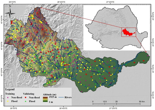
The study area is located in the south-eastern part of Romania and covers an area of 5350 km². The altitudes of the study area, which are in a relatively high range, between 1 m and 1925 m, highlight necessary relief energy that favours the propagation of floods from the upper areas to those at low altitudes. The high slopes, higher than 25°, in the upper part of the basin corroborated with the flat surfaces in the lowlands part, is another element that certifies the potential for flood propagation in the upper area and the potential for flow accumulation in the lower part of the basin. From the geological point of view, in the mountain region of the study area, deposits of the internal Cretaceous flysch can be encountereddeposits of the internal Cretaceous flysch can be encountered while in the hilly area dominates the Miocene Sarmato-Pliocene deposits. The plain region is characterized by sedimentary rocks like clays, gravels, and sands. The geological structure corroborated with exogenous factors determines the occurrence of several geomorphological phenomena like gully erosion and landslides which are closely related to the flash-flood phenomena. At the study area level, the mean annual precipitation around 750 mm/year, while the maximum rainfall in 24 hours equal to 115.4 mm occurred on 12 July 1969 at Lăcăuți meteorological station (Minea 2013). From the hydrological point of view, the highest the most important event occurred in 1975 when, after a rainfall, the Buzău river's discharge, the main collector in the hydrographic basin, reached to 2100 m³/s at Măgura hydrometric station. Other important flood events on the main tributary rivers occurred in 2005 when the maximum discharge values came 56.2 m³/s on Câlnău river and 54 m³/s on Slănic river (Negru 2010). The land use, including forests (40.7%), arable land (30.9%), and built-up areas (4.6%), are other environmental variables that highly influence the flooding potential across the study area.

3. Data

3.1. Flood inventory

It is unanimously accepted that the accurate prediction of the areas that may be affected by a phenomenon in the future must be based on the characteristics of the factors that have favored the production of that phenomenon in the past (Ali et al. 2020; Yariyan et al). Thus, in the present study, the inventory of the locations affected by the floods in the period 1990 − 2020 was carried out, being taken into account only those events that caused damages within the socio-economic elements. A number of 205 flood locations were quantified over the research zone (Figure 1). The General Inspectorate archives for Emergency Situations and National Administration of Romanian Waters were consulted to identify the flood locations. To increase the performance of the applied models, another data set representing 205 non-flood locations was generated. The 2 data sets were divided into training data set (70%) and validating data set (30%). This ratio between the training data set and validating data set is recommended by most researchers focused on natural hazards susceptibility assessment (Lee et al. 2017; Kalantar et al. 2018; Ali et al. 2020; Pham et al. 2020a). Moreover, in a study related to the natural hazards susceptibility computation, Sahin et al. (2020) demonstrated that the results achieved with the ratio of 70:30 between the training and validation data sets were characterized by a lower error than the results achieved by applying other ratios.

Figure 1. Study area location.

3.2. Flood conditioning factors

While the flood locations will be the dependent variable in estimating the flood susceptibility, a number of 12 flood predictors will be used as explanatory variables, and their spatial distribution will be based on the flood exposure values. It is worth stating that the following predictors were selected following a meticulous analysis of the literature (Nguyen et al. 2017; Tang et al. 2020; Costache et al. 2020c): slope, altitude, aspect, TPI, TWI, convergence index, plan curvature, hydrological soil groups, land use, distance from rivers, lithology and rainfall. The first 7 mentioned flood predictors, which are also morphometric indices, were derived from the Digital Elevation Model (DEM) extract from the Shuttle Radar Topographic Mission (SRTM) 30 m. It is worth noting that, at the present moment, for perimeter covered the study area, another DEM with a high resolution of 30 m is not available. Also, the use of the DEM extracted from the SRTM 30 m database has been proved a high-quality solution for the previous studies focused on the same research topic (Dahri and Abida 2017; Sahana et al. 2020). Therefore, all the 7 morphometric factors will have the exact spatial resolution of 30 × 30 m. In order to involve the other 5 flood predictors in the analysis, their associated GIS layers were directly derived or converted into raster layers with the exact spatial resolution of 30 × 30 m. The most accurate data sources available at this moment at the study area level were used for all flood predictors. A short description of each flood predictor is given below.

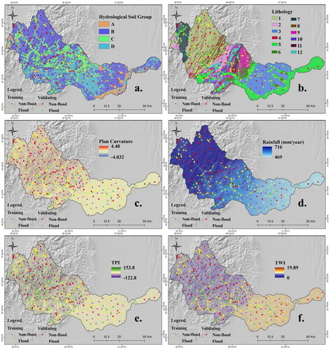
The slope gradient is an essential characteristic of the ground surface, which highly contributes to surface runoff and flow accumulation. The slope factor was derived from DEM, and his values range between 0° and 55.96° (Figure 2a). The elevation is another critical factor in defining the exposure to floods because it highlights the differences between high areas where surface runoff is formed and the low areas where it accumulates (Costache 2019a). Within the study area, the altitudes range from 1 m to 1925 m (Figure 2b). The aspect is another predictor with an important influence on flood occurrence (Figure 2c). According to Costache et al. (2020c), the Eastern and South-Eastern slopes cover 30% of the study area. Convergence index is a morphometric indicator that highlights the valleys perimeters with negative values and the interfluvial areas with positive ones (Figure 2d). Natural environmental response to human activities (Feng et al. 2020; Zhang et al. 2021). Land use is one of the most important flood predictors since it influences the velocity of surface runoff due to Manning roughness coefficients' different values. The arable lands and forests account for around 75% of the study area (Figure 2e). The maximum distance from rivers within Buzau river catchment reaches 10648 m (Figure 2f). The closer they are to the rivers, the more prone the areas are to floods . Hydrological Soil Group (HSG) influences the velocity of water infiltration and, finally, the accumulation potential at the ground surface (Norbiato et al. 2008; Zhang et al. 2019). All the four HSGs can be found within the study area, and HSG B (55%) covers the most extensive surfaces (Figure 3a). Along with the influence on water infiltration, lithology also has contributed to the shape of river valley morphology. Buzău river basin has 12 lithological categories (Figure 3b) on which the highest percentage is covered by flysch (25%). Plan curvature is used to subdivide the hillslopes into concave, convex and planar regions with the plan curvature equal to 0. In our study area, the plan curvature values range from −4.032 to 4.48 (Figure 3c). Rainfall is the environmental factor that determines the flood genesis. Within the study area, the multiannual average rainfall range from 469 mm to 716 mm (Figure 3d). Topographic Position Index (TPI) is a morphometric variable that highlights the difference of the elevation between a specific cell and the neighbouring cells (Pham et al. 2020b). In the case of the present research area, the maximum TPI value is equal to 153.8 while the minimum one is −122.8 (Figure 3e). TWI values indicate the areas from the ground surface where the flow accumulation is favored from a morphometric perspective (Tang et al. 2020). In the present study, the TWI values range from 0 to 19.89 (Figure 3f).

Figure 2. Flood conditioning factors (a. Slope; b. Elevation; c. Aspect; d. Convergence Index; e. Land use; f. Distance from rivers).

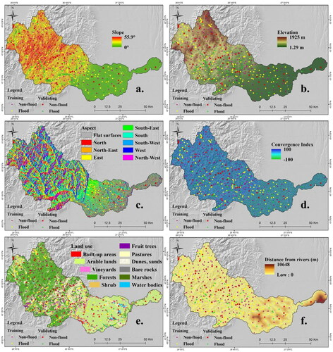
Figure 3. Flood conditioning factors (a. Hydrological Soil Group; b. Lithology; c. Plan curvature; d. Rainfall; e. TPI; f. TWI).

4. Methods background

4.1. Support vector machine (SVM)

In terms of flood susceptibility modeling, the SVM algorithm uses the flood predictors' nonlinear transformations in higher dimensional feature space (Yilmaz 2010; Ghorbanzadeh et al. 2019; Nguyen et al. 2019). Based on the statistical learning theory, in the first stage, SVM is trained with a training dataset. The first advantage of the SVM model is that this model can reduce the error test and the model complexity. In this regard, the SVM method tries to find an optimal hyper-plane that could separate the support vectors (flood and non-flood locations) (Kalantar et al. 2018). In most situations, the hyper-plane will be defined by a non-linearly surface. In this case, the following mathematical expression will be employed to classify the data set (Costache et al. 2020c): (1) $$f\left(x\right)=\sum _{i=1}^n\left({\alpha }_i-{\alpha }_i^{\mathrm{*}}\right)K\left(x_i,x\right)+b$$(1) where α_i and α_i* represent the Lagrange multipliers (α_i ≥ 0, α_i* ≤ C), K(x_i, x_j) represents the kernel function, and b represents the offset of the hyper-plane from the origin.

4.2. J48 decision trees

J48 Decision Trees algorithm, which includes a root node, internal nodes, and leaf nodes, will be used in the present article to create a binary classification of the flood predictors into the flood and non-flood pixels (Tien Bui et al. 2012). The root node will contain all the input data, the internal nodes will ensure the application of the decision function, while the leaf nodes are associated with the output data (Pham et al. 2017b). J48 training process is carried out in 2 main phases as follows: i) construction of classification tree; ii) pruning the classification tree. In the first stage, at the root node will be determined the input data having the gain ratio with the highest value. Based on the root node values, the splitting procedure will be implemented in the case of the training dataset to create sub-nodes. The second stage will consist of the generation of the individual gain ratio for each sub-node. The classification of flood predictors into flood or non-flood will be carried out, taking into account the gain ratio associated with each sub-node (Pham et al. 2017b).

4.3. Adaptive neuro-fuzzy inference system (ANFIS)

ANFIS is a hybrid algorithm proposed by Jang (1993) and is generated through Artificial Neural Network and Fuzzy Logic (FL) method. ANFIS represents a data-driven algorithm characterized by a self-learning function that can be run without input conditions (Gao et al. 2019; Costache 2019a; Ghorbanzadeh et al. 2020). The FL is the fuzzy inference system method (FIS) to transform a specific set of inputs into an output (Polykretis et al. 2019). The fuzzy if-then rule represents a way to describe a particular problem in linguistic terms. The if-then rules have the following form and belong to Takagi and Sugeno’s type (Celikyilmaz and Turksen 2009): (2) $$\text{Rule}\mathrm{}1:\mathrm{}\text{if}\mathrm{}x\mathrm{}\text{is}\mathrm{}{A}_1\mathrm{}\text{and}\mathrm{}y\mathrm{}\text{is}\mathrm{}{B}_1,\mathrm{}\text{then}\mathrm{}{f}_1=p_{1}x+q_{1}y+r_1$$(2) (3) $$\text{Rule}\mathrm{}2:\mathrm{}\text{if}\mathrm{}x\mathrm{}\text{is}\mathrm{}{A}_{2\mathrm{}}\text{and}\mathrm{}y\mathrm{}\text{is}\mathrm{}{B}_2,\mathrm{}\text{then}\mathrm{}{f}_2=p_{2}x+q_{2}y+r_2$$(3) where A₁, A₂, B₁ and B₂ are membership functions (MFs) for the inputs x and y, and p_ix, q_iy and r_ij (i, j = 1, 2) are consequent parameters (Costache 2019a; Moayedi et al. 2019a, 2019b).

The ANFIS model structure contained six layers and was described in a detailed manner by Costache (2019a).

4.4. Random forest

Random Forest (RF) is a prevalent decision trees-based method in natural hazards researches whose main aim is the classification and prediction topics ( ; Chen et al. 2021). This method was introduced by Breiman (2001) and dincluded integration of the random subspace model with bagging ensemble learning (Chen et al. 2020). The following three-stage characterize the RF procedure: i) defining and resampling the training data several times; ii) selection of random features set associated to each re-sample; iii) assigning a decision tree for each to resample and random features set; iv) creation of a single decision tree through the aggregation of decision tree assigned to each resample.

4.5. Multilayer perceptron

Multilayer Perceptron (MLP) is a neural network with a structure composed of three layers, among which one is an intermediate layer that is not directly connected to input and output data. The input data is distributed towards the neural network's middle or hidden layer using the input layer units (Pham et al. 2017a). Further, the output layer will provide many output signals to respond to the information received from the intermediate layer (Dodangeh et al. 2020). In the present study, the number of input neurons included in the input layer will be the same as the number of flood predictors. In contrast, the output layer will contain two neurons associated with the flood and non-flood points. The number of hidden neurons will be calculated according to the following procedure (Sheela and Deepa 2013; Costache and Bui 2019): 2*Ni + 1, where N is equal to the number flood predictors.

4.6. Alternating decision tree

In the Alternating Decision Tree (ADT) model, the Boosting algorithm improves the initial decision tree method (Wu et al. 2020). ADT contains a first layer associated with the decision nodes, which impose a predicate condition. The second layer of ADT contains multiple prediction nodes with a single number (Hong et al. 2015). In the present case study, the ADT will be involved in calculating flood predictors values as flood and non-flood pixels. Thus, the information associated with the spatial distribution of flood and non-flood points and flood predictors values will be used as input in the ADT model, whose functionality is described by the following relations: (4) $$a=0.5\mathrm{*}\ln \frac{W_{+}{(c}_1\cap c_2)}{W_{-}{(c}_1\cap c_2)},\mathrm{}b=0.5\mathrm{*}\ln \frac{W_{+}{(c}_1\cap \overline{c_2})}{W_{-}{(c}_1\cap \overline{c_2})}$$(4) (5) $$z_t(c_1{c}_2)=2\sqrt{W_{+}{(c}_1\cap c_2)\mathrm{*}{W}_{-}{(c}_1\cap c_2)}+\sqrt{W_{+}{(c}_1\cap \overline{c_2}){\mathrm{*}W}_{-}{(c}_1\cap \overline{c_2})}+W(\overline{c_2})$$(5) where W indicates the sum of the values provided by the prediction nodes, c₁ is a precondition, c₂ is the base condition, a and b are 2 real numbers.

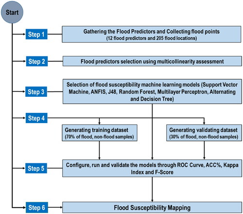
The methodological steps followed in the present research are highlighted in Figure 4.

Figure 4. Methodological flowchart.

5. Results

5.1. Flood predictors selection using multicollinearity assessment

The multicollinearity among the flood predictors was estimated in order to avoid the unnecessary information to be used in the modeling. Thus, the values of Tolerance (TOL) range between 0.248, for altitude, and 0.935, for aspect predictor. The other multicollinearity indicator, Variance Inflation (VIF), has a minimum of 1.070, in the case of aspect, and a maximum of 4.032, in Altitude (Table 1). Therefore, it can be assumed that serious multicollinearity is not present among the flood predictors, and all 12 variables will be taken into account in the modeling process.

Table 1. The multicollinearity analysis for flood predictors.

Flood predictor	Tolerance	VIF
Elevation	0.248	4.032
Aspect	0.935	1.070
Slope	0.340	2.939
TPI	0.465	2.152
TWI	0.374	2.675
Convergence index	0.490	2.041
Distance to rivers	0.760	1.316
Rainfall	0.251	3.984
Hydrological Soil Group	0.710	1.408
Lithology	0.602	1.662
Land use	0.341	1.743
Plan curvature	0.608	1.644

5.2. Flood susceptibility models performance

Once established the flood predictors, their values were extracted to the flood and non-flood locations using GIS software. Further, the records of flood and non-flood pixels from the training sample and flood predictors' values were used to run the six machine learning models. The model’s performances were evaluated using several statistical metrics presented in Table 2. Also, it should be noted that the statistical metrics were calculated for both training and validation samples. In the case of the training sample, the high value of Accuracy was achieved by the RF model (0.971), followed by ANFIS (0.939), ADT (0.93), SVM (0.904), MLP (0.9), and J48 (0.825). In terms of validation sample, the accuracy of the RF algorithm was again the best (0.973), followed by ANFIS (0.938), ADT (0.938), MLP (0.902), SVM (0.902), and J48 (0.83). The accuracy values that exceed the threshold of 0.8 confirm that all the data mining models obtained outstanding performances.

Table 2. Validation of training and validation data using accuracy, sensitivity, specificity, F-Score, and Kappa.

	Metric	SVM	J48	ANFIS	RF	MLP	ADT
Training data	TN	125	115	132	135	125	132
	FP	15	25	8	5	15	8
	FN	12	24	9	3	13	10
	TP	128	116	131	137	127	130
	Accuracy	0.904	0.825	0.939	0.971	0.900	0.93
	Sensitivity	0.914	0.829	0.936	0.979	0.907	0.928
	Specificity	0.893	0.821	0.943	0.964	0.893	0.942
	F-Score	0.905	0.826	0.939	0.972	0.901	0.935
	Kappa	0.807	0.650	0.879	0.943	0.800	0.871
Validation data	TN	50	46	53	54	50	53
	FP	6	10	3	2	6	3
	FN	5	9	4	1	5	4
	TP	51	47	52	55	51	52
	Accuracy	0.902	0.830	0.938	0.973	0.902	0.938
	Sensitivity	0.911	0.839	0.929	0.982	0.911	0.929
	Specificity	0.893	0.821	0.946	0.964	0.893	0.946
	F-Score	0.903	0.832	0.937	0.973	0.903	0.937
	Kappa	0.804	0.661	0.875	0.946	0.804	0.875

5.3. Flood susceptibility mapping and validation

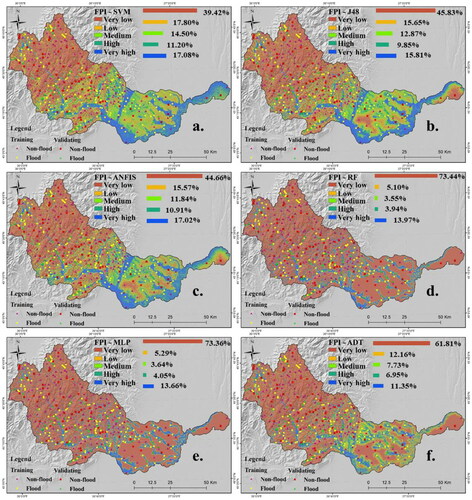
The classification of each flood predictor pixels into flood and non-flood categories allowed the computation of flood susceptibility maps for each machine learning model. The results provided by the SVM model highlights a surface of 39.42% of the study area with a very low flood susceptibility, 17.8% of the study area with a low flood susceptibility, 14.5% with a medium flood susceptibility, and 28.28% with a high and very high flood exposure degree (Figure 5a). With the help of the J48 algorithm, it was found out that 45.83% of the study area has a very low flood susceptibility, 15.65% has a low flood susceptibility, 12.87% has a medium flood susceptibility, while over 26% of the research area has a high and very high flood susceptibility (Figure 5b). The application of the ANFIS model revealed that a very low flood susceptibility covers 44.66% of Buzău catchment, 15.57% is covered by a low flood susceptibility, 11.84% has a medium flood susceptibility. In comparison, the high and very high flood susceptibility is spread on 27.93% of the research area (Figure 5c). RF model highlights the following results: 73.44% for very low flood susceptibility, 5.1% for low flood susceptibility, 3.55% for medium flood susceptibility, and 17.91% for very high flood susceptibility (Figure 5d). According to the MLP model, 73.36% of Buzău catchment falls in very low flood susceptibility, 5.29% has a low flood susceptibility, 3.64% has a medium flood susceptibility 17.71% is characterized by a high and very high flood susceptibility (Figure 5e). The use of ADT shows that 61.81% of the research area has a very low flood exposure, 12.16% has a low flood susceptibility, 7.73% has a medium flood susceptibility. In comparison, 18.3% has high and very high exposure to floods (Figure 5f).

Figure 5. Flood Susceptibility Maps (a. FPI-SVM; b. FPI-J48; c. FPI-ANFIS; d. FPI-RF; e. FPI-MLP; f. FPI-ADT).

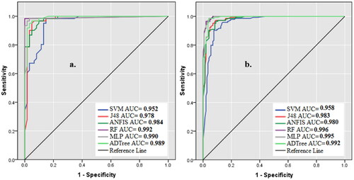
The use of ROC for results validation highlights that the highest AUC in terms of Success Rate was achieved by the RF model (0.996), followed by MLP (0.995), ADT (0.992), J48 (0.983), ANFIS (0.98), and SVM (0.958) (Figure 6a). The highest prediction ability of the models, measured with the help of AUC - Prediction Rate, belongs also to the RF model (0.992), followed by MLP (0.99), ADT (0.989), ANFIS (0.984), and SVM (0.952) (Figure 6b).

Figure 6. ROC Curve (a. Success Rate; b. Prediction Rate).

6. Discussions

Given the events of severe floods in recent years in Romania, assessing the susceptibility to these hazards in the most vulnerable regions of this country is an activity that cannot be omitted and postponed. The machine learning algorithms provide a very accurate assessment of flood susceptibility and, therefore, the use of state-of-the-art models became indispensable (Azareh et al. 2019). Thus, on the Buzau river basin, a very accurate estimation of flood susceptibility was made through 6 machine learning models that provided also results with high accuracy in other previous studies focused on natural hazards susceptibility assessment (Zare et al. 2013; Hong et al. 2015; Kalantar et al. 2018; Polykretis et al. 2019; Chen et al. 2020). It should be noted that the maximum accuracy of the models applied in this study, obtained by RF (AUC = 0.996), exceeded the ultimate accuracy of the models used by Costache et al. (2020c), which also estimated the flood susceptibility within the Buzau river basin. The maximum accuracy achieved by Costache et al. (2020c) was equivalent to an AUC equal to 0.979 and was associated with the application of Support Vector Machine - Index of Entropy ensemble. Moreover, all the models applied in the present research obtained, in terms of Prediction Rate, higher accuracy than the models used by Popa et al. (2019) in a study focused on the same study area. In the present study, there is a more pronounced highlighting of regions with a very low potential for flooding that covers between 39% and 74% of the Buzău river basin, compared to areas with very low susceptibility obtained by Costache et al. (2020c), which cover an area between 19.35% and 28.62%, and by Popa et al. (2019), which spreads 6%. Also, in the case of the present study, the areas with a medium susceptibility are limited to a maximum of 14.5% compared to the previous studies in which they reached a maximum of 43% of the total. This shows that the extreme values ​​of flood susceptibility are better highlighted in the present case study than in the studies done by Popa et al. (2019) and Costache et al. (2020c). These differences between the 2 studies conducted on the same river basin can be explained by the fact that Popa et al. (2019) and Costache et al. (2020c) classified the continuous values ​​flood predictors into several classes before introducing them into machine learning models, while in the case of the present study unclassified factors were used. In both studies, it can be remarked the presence of high flood exposure along to the major river valleys, in the depression’s areas, or over the surfaces with a low slope angle.

As was demonstrated in the previous works related to the natural hazards susceptibility assessment, the parameters of the present paper's models have a significant influence on the final results obtained. For example, in the case of Multilayer Perceptron Neural Network, a strong impact in the results accuracy is held by the back-propagation function, whose main scope is to reduce as much as possible the classification error between during the training phase (Saha et al. 2021). Moreover, for the SVM algorithm, the model complexity and precision is an influence in a high measure by the cost parameter (Oh et al. 2018), while the Random Forest model accuracy is highly determined by the hyperparameters represented by a specific number of decision trees (Lee et al. 2017).

7. Conclusions

Land use planning and flood risk management require a good knowledge of the areas prone to significant flood events. Buzău river basin represents a region from Romania territory which should frequently face flood hazards. In this situation, an accurate flood susceptibility map will represent a valuable tool for the authorities in charge of flood mitigation actions. In this study, six machine-learning models were trained to achieve the highest accurate flood susceptibility maps across Buzău river basin. Twelve flood predictors, selected after multicollinearity assessment, and 205 flood and 205 non-flood locations were involved in the model training and validating the resulting maps. The most accurate model was Random Forest, which achieved an AUC of 0.996 while the lowest accuracy was associated with the J48 model with an AUC of 0.978. These very high AUC values can be considered proof that the DEM at 30 m, removed from SRTM database, represents a reliable source for the derivation of morphometrical indicators used as flood predictors. Therefore, we can conclude that the present results can be reliable tools for governmental decision factors. The algorithms' very high accuracy can also represent a guarantee for other researchers that can use them to estimate the flood susceptibility in different research areas.

Acknowledgments

We would like to thank three anonymous reviewers for their valuable comments. Open Access Funding by the Austrian Science Fund (FWF).

Disclosure statement

No potential conflict of interest was reported by the author(s).

Data availability

The data that support the findings of this study are available on request from the authors.

Funding

This research is partly funded by the Open Access Funding of Austrian Science Fund (FWF) through the GIScience Doctoral College (DK W 1237-N23).

Additional information

Funding

This research is partly funded by the Open Access Funding of Austrian Science Fund (FWF) through the GIScience Doctoral College (DK W 1237-N23).

References

- Alam Z, Sun L, Zhang C, Su Z, Samali B. 2021. Experimental and numerical investigation on the complex behaviour of the localised seismic response in a multi-storey plan-asymmetric structure. Struct Infrastruct Eng. 17(1):86–102.
- Alam Z, Zhang C, Samali B. 2020. Influence of seismic incident angle on response uncertainty and structural performance of tall asymmetric structure. Struct Design Tall Spec Build. 29(12):1750.
- Albano R, Mancusi L, Abbate A. 2017. Improving flood risk analysis for effectively supporting the implementation of flood risk management plans: The case study of “Serio” Valley. Environ Sci Policy. 75:158–172.
- Ali SA, Parvin F, Pham QB, Vojtek M, Vojteková J, Costache R, Linh NTT, Nguyen HQ, Ahmad A, Ghorbani MA. 2020. GIS-based comparative assessment of flood susceptibility mapping using hybrid multi-criteria decision-making approach, naïve Bayes tree, bivariate statistics and logistic regression: A case of Topľa basin. Slovakia. Ecol Indic. 117:106620.
- Arabameri A, Rezaei K, Cerdà A, Conoscenti C, Kalantari Z. 2019. A comparison of statistical methods and multi-criteria decision making to map flood hazard susceptibility in Northern Iran. Sci Total Environ. 660:443–458.
- Azareh A, Rafiei Sardooi E, Choubin B, Barkhori S, Shahdadi A, Adamowski J, Shamshirband S. 2019. Incorporating multi-criteria decision-making and fuzzy-value functions for flood susceptibility assessment. Geocarto Int:1–21.
- Breiman L. 2001. Random forests. Mach. Learn. 45(1):5–32.
- Brillinger M, Dehnhardt A, Schwarze R, Albert C. 2020. Exploring the uptake of nature-based measures in flood risk management: Evidence from German federal states. Environ Sci Policy. 110:14–23.
- Celikyilmaz A, Turksen IB. 2009. Modeling uncertainty with fuzzy logic. Stud. Fuzziness Soft Comput. 240:149–215.
- Chao L, Zhang K, Li Z, Zhu Y, Wang J, Yu Z. 2018. Geographically weighted regression based methods for merging satellite and gauge precipitation. J Hydrol. 558:275–289.
- Chen Y, He L, Guan Y, Lu H, Li J. 2017. Life cycle assessment of greenhouse gas emissions and water-energy optimization for shale gas supply chain planning based on multi-level approach: Case study in Barnett, Marcellus, Fayetteville, and Haynesville shales. Energy Convers Manage. 134:382–398.
- Chen Y, Li J, Lu H, Yan P. 2021. Coupling system dynamics analysis and risk aversion programming for optimizing the mixed noise-driven shale gas-water supply chains. J Cleaner Prod. 278:123209.
- Chen W, Li Y, Xue W, Shahabi H, Li S, Hong H, Wang X, Bian H, Zhang S, Pradhan B, et al. 2020. Modeling flood susceptibility using data-driven approaches of naïve bayes tree, alternating decision tree, and random forest methods. Sci Total Environ. 701:134979.
- Chen W, Zhang S, Li R, Shahabi H. 2018. Performance evaluation of the GIS-based data mining techniques of best-first decision tree, random forest, and naïve Bayes tree for landslide susceptibility modeling. Sci Total Environ. 644:1006–1018.
- Chen Y, Zheng W, Li W, Huang Y. 2021. Large group activity security risk assessment and risk early warning based on random forest algorithm. Pattern Recog Lett. 144:1–5.
- Costache R. 2019b. Flash-Flood Potential assessment in the upper and middle sector of Prahova river catchment (Romania). A comparative approach between four hybrid models. Sci Total Environ. 659:1115–1134.
- Costache R. 2019a. Flood susceptibility assessment by using bivariate statistics and machine learning models-a useful tool for flood risk management. Water Resour Manage. 33(9):3239–3256.
- Costache R. 2019c. Flash-flood Potential Index mapping using weights of evidence, decision Trees models and their novel hybrid integration. Stoch Environ Res Risk Assess. 33(7):1375–1402.
- Costache R, Bui DT. 2019. Spatial prediction of flood potential using new ensembles of bivariate statistics and artificial intelligence: A case study at the Putna river catchment of Romania. Sci Total Environ. 691:1098–1118.
- Costache R, Ngo PTT, Bui DT. 2020a. Novel ensembles of deep learning neural network and statistical learning for flash-flood susceptibility mapping. Water. 12(6):1549.
- Costache R, Pham QB, Avand M, Linh NTT, Vojtek M, Vojteková J, Lee S, Khoi DN, Nhi PTT, Dung TD. 2020b. Novel hybrid models between bivariate statistics, artificial neural networks and boosting algorithms for flood susceptibility assessment. J Environ Manage. 265:110485.
- Costache R, Popa MC, Bui DT, Diaconu DC, Ciubotaru N, Minea G, Pham QB. 2020c. Spatial predicting of flood potential areas using novel hybridizations of fuzzy decision-making, bivariate statistics, and machine learning. J Hydrol. 585:124808.
- Dahri N, Abida H. 2017. Monte Carlo simulation-aided analytical hierarchy process (AHP) for flood susceptibility mapping in Gabes Basin (southeastern Tunisia). Environ. Earth Sci. 76:302.
- Dat TT, Tri DQ, Truong DD, Hoa NN. 2019. Application of mike flood model in inundation simulation with the dam-break scenarios: a case study of Dak-Drinh Reservoir in Vietnam. Int J Earth Sci Eng. 12:60–70.
- Didovets I, Krysanova V, Bürger G, Snizhko S, Balabukh V, Bronstert A. 2019. Climate change impact on regional floods in the Carpathian region. J Hydrol Reg Stud. 22:100590.
- Dodangeh E, Choubin B, Eigdir AN, Nabipour N, Panahi M, Shamshirband S, Mosavi A. 2020. Integrated machine learning methods with resampling algorithms for flood susceptibility prediction. Sci Total Environ. 705:135983.
- Douinot A, Roux H, Garambois P-A, Larnier K, Labat D, Dartus D. 2016. Accounting for rainfall systematic spatial variability in flash flood forecasting. J Hydrol. 541:359–370.
- Feng S, Lu H, Tian P, Xue Y, Lu J, Tang M, Feng W. 2020. Analysis of microplastics in a remote region of the Tibetan Plateau: Implications for natural environmental response to human activities. Sci Total Environ. 739:140087.
- Gao W, Moayedi H, Shahsavar A. 2019. The feasibility of genetic programming and ANFIS in prediction energetic performance of a building integrated photovoltaic thermal (BIPVT) system. Sol Energy. 183:293–305.
- Gharaei-Manesh S, Fathzadeh A, Taghizadeh-Mehrjardi R. 2016. Comparison of artificial neural network and decision tree models in estimating spatial distribution of snow depth in a semi-arid region of Iran. Cold Reg Sci Technol. 122:26–35.
- Ghorbanzadeh O, Blaschke T, Aryal J, Gholaminia K. 2020. A new GIS-based technique using an adaptive neuro-fuzzy inference system for land subsidence susceptibility mapping. J Spatial Sci. 65(3):401–417.
- Ghorbanzadeh O, Blaschke T, Gholamnia K, Meena SR, Tiede D, Aryal J. 2019. Evaluation of different machine learning methods and deep-learning convolutional neural networks for landslide detection. Remote Sens-Basel. 11(2):196.
- Giang PQ, Trang NTM, Anh TTH, Binh NT. 2020. Prediction of economic loss of rice production due to flood inundation under climate change impacts using a modeling approach: A case study in Ha Tinh Province, Vietnam. Clim Change. 6:52–63.
- Haer T, Husby TG, Botzen WW, Aerts JC. 2020. The safe development paradox: An agent-based model for flood risk under climate change in the European Union. Glob Environ Change. 60:102009.
- Hong H, Pradhan B, Xu C, Bui DT. 2015. Spatial prediction of landslide hazard at the Yihuang area (China) using two-class kernel logistic regression, alternating decision tree and support vector machines. Catena. 133:266–281.
- Hu J, Zhang H, Liu L, Zhu X, Zhao C, Pan Q. 2020a. Convergent multiagent formation control with collision avoidance. IEEE Trans Robot. 36(6):1805–1814.
- Hu J, Zheng B, Wang C, Zhao C, Hou X, Pan Q, Xu Z. 2020b. A survey on multi-sensor fusion based obstacle detection for intelligent ground vehicles in off-road environments. Front Inform Technol Electron Eng. 21(5):675–692.
- Jang J-S. 1993. ANFIS: adaptive-network-based fuzzy inference system. IEEE Trans Syst Man Cybern. 23(3):665–685.
- Jiang Q, Shao F, Gao W, Chen Z, Jiang G, Ho Y-S. 2018. Unified no-reference quality assessment of singly and multiply distorted stereoscopic images. IEEE Trans Image Process. 28(4):1866–81.
- Jiang Q, Shao F, Lin W, Gu K, Jiang G, Sun H. 2018. Optimizing multistage discriminative dictionaries for blind image quality assessment. IEEE Trans Multimedia. 20(8):2035–2048.
- Johann G, Leismann M. 2017. How to realise flood risk management plans efficiently in an urban area–the S eseke project. J Flood Risk Manage. 10(2):173–181.
- Kalantar B, Pradhan B, Naghibi SA, Motevalli A, Mansor S. 2018. Assessment of the effects of training data selection on the landslide susceptibility mapping: a comparison between support vector machine (SVM), logistic regression (LR) and artificial neural networks (ANN). Geomat Nat Hazards Risk. 9(1):49–69.
- Khalfallah CB, Saidi S. 2018. Spatiotemporal floodplain mapping and prediction using HEC-RAS-GIS tools: Case of the Mejerda river. Tunisia. J Afr Earth Sci. 142:44–51.
- Khosravi K, Pham BT, Chapi K, Shirzadi A, Shahabi H, Revhaug I, Prakash I, Bui DT. 2018. A comparative assessment of decision trees algorithms for flash flood susceptibility modeling at Haraz watershed, northern Iran. Sci Total Environ. 627:744–755.
- Kocaman S, Tavus B, Nefeslioglu HA, Karakas G, Gokceoglu C. 2020. Evaluation of floods and landslides triggered by a meteorological catastrophe (Ordu, Turkey, August 2018) using optical and radar data. Geofluids. 2020:1–18.
- Lee S, Kim J-C, Jung H-S, Lee MJ, Lee S. 2017. Spatial prediction of flood susceptibility using random-forest and boosted-tree models in Seoul metropolitan city. Korea. Geomat Nat Hazards Risk. 8(2):1185–1203.
- Leon AS, Goodell C. 2016. Controlling Hec-Ras using Matlab. Environ Model Softw. 84:339–348.
- Li B-H, Liu Y, Zhang A-M, Wang W-H, Wan S. 2020. A survey on blocking technology of entity resolution. J Comput Sci Technol. 35(4):769–793.
- Li C, Sun L, Xu Z, Wu X, Liang T, Shi W. 2020. Experimental investigation and error analysis of high precision FBG displacement sensor for structural health monitoring. Int J Str Stab Dyn. 20(6):2040011.
- Li T, Xu M, Zhu C, Yang R, Wang Z, Guan Z. 2019. A deep learning approach for multi-frame in-loop filter of HEVC. IEEE Trans Image Process. 28(11):5663–5678.
- Li J, Zhang B, Mu C, Chen L. 2018. Simulation of the hydrological and environmental effects of a sponge city based on MIKE FLOOD. Environ Earth Sci. 77:32.
- Löwe R, Urich C, Domingo NS, Mark O, Deletic A, Arnbjerg-Nielsen K. 2017. Assessment of urban pluvial flood risk and efficiency of adaptation options through simulations–A new generation of urban planning tools. J Hydrol. 550:355–367.
- Lu H, Guan Y, He L, Adhikari H, Pellikka P, Heiskanen J, Maeda E. 2019b. Patch aggregation trends of the global climate landscape under future global warming scenario. Int J Climatol. 40(5):2674–2685.
- Lu H, Tian P, He L. 2019a. Evaluating the global potential of aquifer thermal energy storage and determining the potential worldwide hotspots driven by socio-economic, geo-hydrologic and climatic conditions. Renewable Sustainable Energy Rev. 112:788–796.
- Markus M, Angel J, Byard G, McConkey S, Zhang C, Cai X, Notaro M, Ashfaq M. 2018. Communicating the impacts of projected climate change on heavy rainfall using a weighted ensemble approach. J Hydrol Eng. 23(4):04018004.
- Ma M, Wang H, Jia P, Liu R, Hong Z, Labriola LG, Hong Y, Miao L. 2018. Investigation of inducements and defenses of flash floods and urban waterlogging in Fuzhou, China, from 1950 to 2010. Nat Hazards. 91(2):803–818.
- Ma X, Zhang K, Zhang L, Yao C, Yao J, Wang H, Jian W, Yan Y. 2021. Data-driven niching differential evolution with adaptive parameters control for history matching and uncertainty quantification. SPE J. 26(02):993–1010.
- Minea G. 2013. Assessment of the flash flood potential of Bâsca River Catchment (Romania) based on physiographic factors. Open Geosci. 5:344–353.
- Moayedi H, Raftari M, Sharifi A, Jusoh WAW, Rashid ASA. 2019a. Optimization of ANFIS with GA and PSO estimating α ratio in driven piles. Eng Comput. 36(1):227.
- Moayedi H, Tien Bui D, Gör M, Pradhan B, Jaafari A. 2019b. The feasibility of three prediction techniques of the artificial neural network, Adaptive neuro-fuzzy inference system, and hybrid particle swarm optimization for assessing the safety factor of cohesive slopes. IJGI. 8(9):391.
- Nachappa TG, Ghorbanzadeh O, Gholamnia K, Blaschke T. 2020. Multi-hazard exposure mapping using machine learning for the State of Salzburg, Austria. Remote Sens-Basel. 12(17):2757.
- Nachappa TG, Piralilou ST, Gholamnia K, Ghorbanzadeh O, Rahmati O, Blaschke T. 2020. Flood susceptibility mapping with machine learning, multi-criteria decision analysis and ensemble using Dempster Shafer Theory. J Hyd:125275, 590 (2020).
- Negru O. 2010. Flood management in Buzău river basin, in: Water Resources from Romania. Vulnerability to the Pressure of Man’s Activities. 16:5–12.
- Nguyen V-N, Bui DT, Ngo P-TT, Nguyen Q-P, Nguyen VC, Long NQ, Revhaug I. 2017. An integration of least squares support vector machines and firefly optimization algorithm for flood susceptible modeling using GIS. Presented at the International Conference on Geo-Spatial Technologies and Earth Resources, Springer, p. 52–64.
- Nguyen H, Bui XN, Tran QH, Moayedi H. 2019. Predicting blast-induced peak particle velocity using BGAMs, ANN and SVM: a case study at the Nui Beo open-pit coal mine in Vietnam. Environ Earth Sci. 78 (15):1–14.
- Norbiato D, Borga M, Degli Esposti S, Gaume E, Anquetin S. 2008. Flash flood warning based on rainfall thresholds and soil moisture conditions: An assessment for gauged and ungauged basins. J. Hydrol. 362(3-4):274–290.
- Oh H-J, Kadavi PR, Lee C-W, Lee S. 2018. Evaluation of landslide susceptibility mapping by evidential belief function, logistic regression and support vector machine models. Geomat Nat Hazards Risk. 9(1):1053–1070.
- Peptenatu D, Grecu A, Simion AG, Gruia KA, Andronache I, Draghici CC, Diaconu DC. 2020. Deforestation and frequency of floods in Romania. In: Water resources management in Romania. Springer, Cham; p. 279–306.
- Pham BT, Avand M, Janizadeh S, Phong TV, Al-Ansari N, Ho LS, Das S, Le HV, Amini A, Bozchaloei SK, et al. 2020a. GIS based hybrid computational approaches for flash flood susceptibility assessment. Water. 12(3):683.
- Pham BT, Bui DT, Pourghasemi HR, Indra P, Dholakia M. 2017a. Landslide susceptibility assesssment in the Uttarakhand area (India) using GIS: a comparison study of prediction capability of naïve bayes, multilayer perceptron neural networks, and functional trees methods. Theor Appl Climatol. 128(1–2):255–273.
- Pham BT, Bui DT, Prakash I. 2017b. Landslide susceptibility assessment using bagging ensemble based alternating decision trees, logistic regression and J48 decision trees methods: a comparative study. Geotech Geol Eng. 35(6):2597–2611.
- Pham BT, Phong TV, Nguyen HD, Qi C, Al-Ansari N, Amini A, Ho LS, Tuyen TT, Yen HPH, Ly H-B, et al. 2020b. A comparative study of Kernel logistic regression, radial basis function classifier, multinomial Naïve Bayes, and logistic model tree for flash flood susceptibility mapping. Water. 12(1):239.
- Polykretis C, Chalkias C, Ferentinou M. 2019. Adaptive neuro-fuzzy inference system (ANFIS) modeling for landslide susceptibility assessment in a Mediterranean hilly area. Bull Eng Geol Environ. 78(2):1173–1187.
- Popa MC, Peptenatu D, Drăghici CC, Diaconu DC. 2019. Flood hazard mapping using the flood and flash-flood potential index in the Buzău River catchment, Romania. Water. 11(10):2116.
- Ren J. 2012. ANN vs. SVM: Which one performs better in classification of MCCs in mammogram imaging. Knowl.-Based Syst. 26:144–153.
- Saha S, Paul GC, Pradhan B, Abdul Maulud KN, Alamri AM. 2021. Integrating multilayer perceptron neural nets with hybrid ensemble classifiers for deforestation probability assessment in Eastern India. Geomat Nat Hazards Risk. 12(1):29–62.
- Sahana M, Rehman S, Sajjad H, Hong H. 2020. Exploring effectiveness of frequency ratio and support vector machine models in storm surge flood susceptibility assessment: A study of Sundarban Biosphere Reserve, India. Catena. 189:104450.
- Sahin EK, Colkesen I, Kavzoglu T. 2020. A comparative assessment of canonical correlation forest, random forest, rotation forest and logistic regression methods for landslide susceptibility mapping. Geocarto Int. 35(4):341–363.
- Sepehri M, Malekinezhad H, Jahanbakhshi F, Ildoromi AR, Chezgi J, Ghorbanzadeh O, Naghipour E. 2020. Integration of interval rough AHP and fuzzy logic for assessment of flood prone areas at the regional scale. Acta Geophys. 68(2):477.
- Shahid S, Wang X-J, Harun SB, Shamsudin SB, Ismail T, Minhans A. 2016. Climate variability and changes in the major cities of Bangladesh: observations, possible impacts and adaptation. Reg Environ Change. 16(2):459–471.
- Sheela KG, Deepa S. 2013. Neural network based hybrid computing model for wind speed prediction. Neurocomputing. 122:425–429.
- Shi K, Tang Y, Liu X, Zhong S. 2017. Secondary delay-partition approach on robust performance analysis for uncertain time-varying Lurie nonlinear control system. Optim Control Appl Meth. 38(6):1208–1226.
- Tang X, Li J, Liu M, Liu W, Hong H. 2020. Flood susceptibility assessment based on a novel random Naïve Bayes method: A comparison between different factor discretization methods. Catena. 190:104536.
- Tehrany MS, Kumar L, Shabani F. 2019. A novel GIS-based ensemble technique for flood susceptibility mapping using evidential belief function and support vector machine: Brisbane, Australia. PeerJ. 7:e7653.
- Thakur B, Parajuli R, Kalra A, Ahmad S, Gupta R. 2017. Coupling HEC-RAS and HEC-HMS in precipitation runoff modelling and evaluating flood plain inundation map. Presented at the World Environmental and Water Resources Congress 2017, p. 240–251.
- Tian P, Lu H, Feng W, Guan Y, Xue Y. 2020. Large decrease in streamflow and sediment load of Qinghai–Tibetan Plateau driven by future climate change: A case study in Lhasa River Basin. CATENA. 187:104340.
- Tien Bui D, Pradhan B, Lofman O, Revhaug I. 2012. Landslide susceptibility assessment in Vietnam using support vector machines, decision tree, and Naive Bayes Models. Math Probl Eng. 2012:1–26.
- Wu Y, Ke Y, Chen Z, Liang S, Zhao H, Hong H. 2020. Application of alternating decision tree with AdaBoost and bagging ensembles for landslide susceptibility mapping. Catena. 187:104396.
- Xue X, Zhang K, Chen Tan K, Feng L, Wang J, Chen G, Zhao X, Zhang L, Yao J. 2020. Affine Transformation-Enhanced Multifactorial Optimization for Heterogeneous Problems. IEEE Trans Cybern.
- Yang Y, Hou C, Lang Y, Sakamoto T, He Y, Xiang W. 2020. Omnidirectional motion classification with monostatic radar system using micro-doppler signatures. IEEE Trans Geosci Remote Sensing. 58(5):3574–3514.
- Yang Y, Yao J, Wang C, Gao Y, Zhang Q, An S, Song W. 2015. New pore space characterization method of shale matrix formation by considering organic and inorganic pores. J Nat Gas Sci Eng. 27:496–503.
- Yilmaz I. 2010. Comparison of landslide susceptibility mapping methodologies for Koyulhisar, Turkey: conditional probability, logistic regression, artificial neural networks, and support vector machine. Environ Earth Sci. 61(4):821–836.
- Zare M, Pourghasemi HR, Vafakhah M, Pradhan B. 2013. Landslide susceptibility mapping at Vaz Watershed (Iran) using an artificial neural network model: a comparison between multilayer perceptron (MLP) and radial basic function (RBF) algorithms. Arab J Geosci. 6(8):2873–2888.
- Zhang Z, Luo C, Zhao Z. 2020. Application of probabilistic method in maximum tsunami height prediction considering stochastic seabed topography. Nat Hazards. 104(3):2511–2530.
- Zhang C, Wang H. 2019. Robustness of the active rotary inertia driver system for structural swing vibration control subjected to multi-type hazard excitations. Appl Sci. 9(20):4391.
- Zhang K, Wang Q, Chao L, Ye J, Li Z, Yu Z, Yang T, Ju Q. 2019. Ground observation-based analysis of soil moisture spatiotemporal variability across a humid to semi-humid transitional zone in China. J Hydrol. 574:903–914.
- Zhang K, Zhang J, Ma X, Yao C, Zhang L, Yang Y, Wang J, Yao J, Zhao H. 2021. History matching of naturally fractured reservoirs using a deep sparse autoencoder. SPE J. 1:1–22
- Zhao J, Liu J, Jiang J, Gao F. 2020. Efficient deployment with geometric analysis for mmWave UAV Communications. IEEE Wireless Commun Lett. 9(7):1115–1119.
- Zuo C, Chen Q, Tian L, Waller L, Asundi A. 2015. Transport of intensity phase retrieval and computational imaging for partially coherent fields: The phase space perspective. Opt Lasers Eng. 71:20–32.