Predicting PM_2.5 levels over the north of Iraq using regression analysis and geographical information system (GIS) techniques

Abstract

Particulate matter (PM_2.5) concentrations are a serious human health concern and global models are the common methods for PM_2.5 particle estimation disregarding the local changes and factors. In this study, a polynomial model for PM_2.5 particles prediction was proposed to examine the correlations among PM_2.5, PM₁₀, and meteorological parameters. The study was carried out in the north of Iraq including two provinces; Kirkuk and Sulaymaniyah. The data gathered from different sources. Two datasets have been used, collected during July 2019 and February 2020. To test our methodology, the model was applied on a small subset of the study area (5.6 km²) inside the Kirkuk province. Datasets (observation and ground truth) were utilized to examine the model. Based on the July 2019 dataset, the mean local R² values were estimated at 0.98 and 0.97 in the north part of Iraq, and inside the Kirkuk province (the small subset), respectively. While based on the February 2020 dataset, the mean local R² values were estimated at 0.98 inside the Kirkuk province. High values of prediction accuracies were obtained by 82% and 96% in July and February, respectively. Moreover, our findings highlighted that the health impacts and air quality varied from moderate to unhealthy in the region.

Keywords:

• PM_2.5
• PM₁₀
• polynomial model
• meteorological parameters
• health impact

1. Introduction

Systematic and long-term air quality monitoring will enable the human for a sustainable plan to reduce and control particle pollution, contaminants, and air pollution. Various studies point out the correlation between the concentration of fine particles and epidemics, where their effect on health is the subject of interest of researchers (He et al. 2001; Marcazzan et al. 2001; Ito et al. 2006; Borrego et al. 2016; Jumaah et al. 2018; Crippa et al. 2019; David et al. 2019). Particulate matter (PM) consists of a mixture of solids and liquids in the atmosphere that is induced to the air by natural and anthropogenic sources (Querol et al. 2004; Hu et al. 2013). Particulate matter 2.5 (PM_2.5) is mainly derived by combustion processes; it contains the elements with a carbon core (with related hydrocarbons and elements), hydrocarbons, and minor atoms shaped by sulfur oxides and nitrogen (Adams et al. 2015). The world health organization (WHO) concluded that PM is itself responsible for the health impacts in related diseases and epidemics and it is supported by toxic traces (Boldo et al. 2006). Due to the complexity of PM composition, it is necessary to control its sources, which contribute to the toxicity components in PM composites (Adams et al. 2015). Given the multiplicity of sources, PM occurs in different physical and chemical patterns and is based on climatic and geographic factors such as air temperature, wetness, radiation, rainfall, land topographic properties, and adjacency of a region to desert areas (Querol et al. 2004).

Air quality data is provided by monitoring stations given as air quality index (AQI) or as other indices with different meanings according to epidemiologic studies. When AQI rises, the contamination of air will be severe and result in adverse effects on the health (Wang and Chen 2017). Currently, air contamination has become one of the main disturbing consequences of urbanization, therefore, air contamination monitoring and assessment are necessary (Jassim and Coskuner 2017). The AQI is a helpful indicator to describe the daily quality of air and it might answer the concerns related to health impacts (Liu 2002). The initial use of AQI was in 1999, and it defines the main six air contaminants (Jassim and Coskuner 2017): fine particles PM_2.5, coarse particles PM₁₀, carbon monoxide (CO), nitrogen dioxide (NO2), ozone (O3), and sulfur dioxide (SO2). Most environmental studies focused on understanding of PM and the ability to predict PM concentrations in a certain region (Chen et al. 2010; Ul-Saufie et al. 2013; Nazif et al. 2016; Ganesh et al. 2018; Jumaah et al. 2018; 2019; Sahu and Patra 2020). Generally, mathematical models are improved to give an effective description of the quantitative or statistical correlation, which exists among the independent factors and particle levels (Tian and Chen 2010). In terms of PM_2.5, the contamination is harmful and threatening especially to human wellness due to the presence of toxic materials, high acids, and their small size permits them to penetrate the respiratory system (Jassim and Coskuner 2017). As a result, various countries in the world described the quality standards to define the values for PM concentration together with specific networks to monitor air quality and condition on the regional and global scales (Manikonda et al. 2016). Additionally, the worldwide measurements of PM are significant to epidemiological studies in terms of the strategy in controlling air quality and forecasting (Van Donkelaar et al. 2006). Given serious environmental pollution problems, air quality monitoring is of great importance in order to be studied and understood (Yang et al. 2018).

In this regard, the researches analyze and measure the correlation of different weather variables and PM_2.5 (Li et al. 2019). Multiple regression analysis is generally used to estimate the dependent parameter based on the impact of independent parameters (Jumaah et al. 2018). The applied regression processes deploy geographical information system (GIS) and statistical methods (e.g., inverse weighted distance (IDW), multiple regression analysis, and polynomial model). It is based on the idea that air quality at a certain place could be influenced by the near and adjacent pollutant sources to that place and would affect the health more than distant sources. Using regression models and spatial data analysis enables us to inspect and describe the spatial relationships (link to the geographical locations) of the variables. Defining the model configuration and estimation of PM_2.5 levels are crucial. Deterministic model building, which clearly describes the contamination, requires usually intense datasets. For instance, one of the important requirements as input data is to define the source of pollution, whereas it might be difficult to determine or quantify the exact origination as a result of pollutant emissions. Tian and Chen (2010) specified that it mainly requires local scale investigations in order to consider the urban areas as an inconstant source of pollution.

Owing to the presence of various software packages to fit the multiple linear models, the least-square fitting of the linear mean function into geostatistical data leads to highly satisfactory results (Gelfand et al. 2010). Geostatistical analysis removes a lot of corresponding errors and restrictions compared to traditional statistics on the basis of the theory of irregular distribution (Setianto and Triandini 2015). In recent times, geospatial analysis using GIS techniques is one of the significant and efficient methods to define air effluent emissions (Tuna and Buluc 2015). Statistical models were grouped by Skidmore (2017) into empirical, numerical, or derived models. The empirical models are based on observations and experiments, where the expectation is accepted, once it is confirmed by the real experience. So, empirical models are considered site-related, due to collecting local data and adequate samples. Therefore, Hvidtfeldt et al. (2018) considered that covering and mapping air contamination exposure for various epidemiological considerations was infeasible and requested to refine the modeling processes. A geographically weighted regression approach applied by Jumaah et al. (2018) using an unmanned arial vehicle (UAV)-based dataset of PM_2.5 correlated to meteorological parameters with 82% to 94% model performance accuracies. Besides a framework of applied air-GIS in research by Hvidtfeldt et al. (2018), it revealed a high level of accuracy for modeling the levels of black carbon which was assessed based on PM_2.5 and PM₁₀. The author noted that the correlation was expected between epidemiological investigations on the health and PM impact. Also, the PM_2.5 levels changes based on seasonal variations were explored by Saxena and Jagdeesh (2019) and it was suggested that additional investigation regarding this anomaly was needed in the region. Consequently, air quality models are progressively essential for public awareness, air quality management, and research purposes. (Donnelly et al. 2019). Traffic-related air pollution makes a significant contribution to the early mortality rates in developed and developing countries and most researches (Chambliss et al. 2014; Silva et al. 2016; Anenberg et al. 2019) highlighted the transport emissions to the exposure of PM_2.5. Also, the effect of some pollutants on Kirkuk air quality was studied by Mohamedali et al. (2020) through mapping the pollutant levels at different places and stations within the city. It was mentioned that the pollutants concentrations exceeded the standards in most of the stations as a consequence of refineries and many traffic crosses. According to Fan et al. (2020), AQI in China slightly increased by 36% when turning to a winter heating system of coal-fired and then it increased the mortality rate up to 14%. Similarly, the exposure to fine particulate (PM_2.5) pollutants in the long term associates with heart disease and higher mortality rates; when the extra risks occur and the ranges excess the specified US agency standards it calls for continuous air contamination reduction (Hayes et al. 2020).

Ultimately, basic statistics and detailed maps of environmental pollutants distribution and regression analysis assist to predict pollutants levels (Fathoni et al. 2013; Tuna and Buluc 2015; Jumaah et al. 2018; Wu et al. 2018; Jumaah et al. 2019; Gui et al. 2020). However, adaptive-neuro-fuzzy inference system is rather precise in forecasting time-series records than the regression approach (Zeinalnezhad et al. 2020) assuming that there are nonlinear and complex components in air contamination modeling. Their study intended to respond that restriction by improving the precision of the day-to-day estimate of contaminants. Using three algorithms (i.e., support vector machine, naive bias, and random forest), air quality predictions for different inputs were analyzed by Bali (2020) with a high prediction accuracy of 99%. Therefore, the precise modeling and estimation of AQI and its relationship with other factors need more investigation.

Recently, some cities in Iraq are at a higher risk of air pollution and this phenomenon occurs widely and frequently in the regions. In terms of air pollution, based on the global air quality service provider (downloaded from https://air-matters.com/), the three cities of Kirkuk, Baghdad, and Najaf exhibited very poor air quality in 2019. In this study, we applied statistical analysis on two types of datasets (observation and ground truth) to predict and examine air pollution in Kirkuk and Sulaymaniyah with enhancement in experimental spatial patterns and exploration in the properties of prediction parameters. The regression processes along with GIS techniques allow for better describing the correlation between the main pollutant and other variables to explain their spatial effects. At this point, the principal goals of this research were: 1) to perform an air quality forecast model in the urban area with PM_2.5 estimation capability in all sites of the study area using linear regression processes, polynomial model, and GIS techniques, 2) to model the spatial variation on a large scale, and 3) to examine the health impacts of particulate matter (PM) on human.

2. Study area, and datasets

2.1. The study area

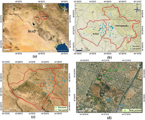
The study area lies in the north of Iraq covering two provinces: Kirkuk (9,679 km²) and Sulaymaniyah (‏20,144 km²). The study area is located between latitudes of 36° 27′ 15" − 36° 37′ 50" N and longitudes of 43° 10′ 37" − 46° 17′ 50" E (Figure 1). Geographically, Iraq is located in Southwest Asia. The average temperature ranges between 50 °C in summer and 0 °C in winter and the annual rainfall varies from 100 to 180 mm. The extreme rainfall happens between December and April, and the mountainous regions in northern Iraq have higher rainfalls than other regions (Al-Bayati and Al-Salihi 2019). Kirkuk climate characterizes as hot semi-arid and extremely hot with dry summers and cold winters (Buraihi and Shariff 2015). The climate of the Sulaymaniyah region is a continental arid climate with dry hot summer, cold winter, and high evaporation in summer due to high temperatures and relatively low humidity (Ali et al. 2015). According to Ajaj et al. (2018), exploratory analysis in Kirkuk by GIS-based spatial technique reported the high incidence of blood diseases patients in 2017. Based on their findings, the extreme incidence of blood disease happened in the southern parts of the city. On the other hand, the minimum prevalence of blood disease was recorded in the northern parts of the city and several quarters in the city center. It raises concerns regarding the environmental health threat and its correlation with air quality in the region as a research subject.

Figure 1. Location of the study area; (a) Iraq, (b) the borders of the two provinces in northern Iraq including train and test points, (c) the experimental area, (d) the experimental and test area including 20 test points (5.6 km²).

2.2. Data and processes

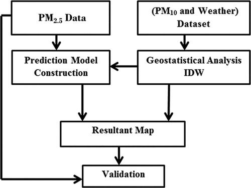
Weather data such as temperature, surface wind speed (m/sec), and humidity (%) significantly improve the model performance (Hu et al. 2013) and meteorological parameters are essential features that affect the PM_2.5 levels (Kong and Tian 2020). Therefore, daily PM_2.5, PM₁₀, temperature, and humidity values of Iraq (July 2019) were acquired from Air Matters and The global air quality service provider (https://air-matters.com/). Besides, some parts of missing data such as PM_2.5 and PM₁₀ for some locations were compiled from Meteoblue, the worldwide local weather information site (https://www.meteoblue.com/). The wind data was gathered from The weather online Ltd. for meteorological services (https://www.weatheronline.co.uk/). All data were in point format and have been collected from nine stations inside and around the study area. Based on the collected datasets, the deployed procedures are described in Figure 2. All collected datasets were processed geo-statistically using ArcGIS version 10.3 and an IDW analysis was applied to the acquired data and existed stations for air quality and weather in the region to obtain continuous and detailed parameters for the region.

Figure 2. The procedures employed in the research.

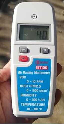
The significance of the IDW method is that a smooth and connected grid can be implemented where the extrapolation of information is created based on the data in the given area (Zaki et al. 2019). It is one of the highest commonly used methods in geoscience calculations due to its simple hypothesis (Sun et al. 2019). The IDW analysis is the finest interpolation process to predict the air contamination state and it is more reliable than the ordinary kriging (OK) or universal kriging (UK) of interpolation methods (Gong et al. 2014; Vorapracha et al. 2015; Jumaah et al. 2019). Interpolation determines the result of the cell at the part that requires descriptive data (Ajaj et al. 2017; Jumaah et al. 2019). In addition, interpolation is created on the concept of a spatial dependent; it measures the proportion of ties dependency amongst the adjacent and separate features (Ajaj et al. 2017). Moreover, a remotely sensed image of moderate resolution imaging spectroradiometer (MODIS) captured on 10 February 2020 was downloaded from NASA satellite erathdata. Additional measurements were applied during February 2020 using Air Quality Multimeter inside Kirkuk at 5.6 km² (Figure 3).

Figure 3. The air quality multimeter.

3. Methodology

3.1. Regression analysis and modelling

Based on all station data, the IDW interpolation was applied. Afterward, 36 input points were randomly chosen within the study area from the outputs of IDW and have been used to build the polynomial model. Besides, the ground truth dataset (southern part of Kirkuk Province at the area of 5.6 km²) was used to validate the model and measure its transferability using the same procedures and parameters as it was applied for those two provinces. Then, Measurements were done manually across a small subset of the region using air quality multimeter. Measurements applied during July 2019 and February 2020.

The PM_2.5 variable was used as the dependent variable and other parameters (i.e., PM₁₀, temperature, humidity, and wind) were used as independent factors. Similarly, for the validation process, the polynomial model to predict PM_2.5 levels also was applied in a subset area. The environmental protection agency (EPA) of the U.S defines the values of AQI and PM_2.5 levels based on their impacts on human health. Table 1 represents the daily PM₁₀, PM_2.5 levels (μg/m³), and AQI modified by EPA as the reference for this study.

Table 1. Daily PM_2.5 and PM₁₀ levels μg/m³ (U.S. Environmental Protection Agency).

PM2.5(μg/m^3)	PM10(μg/m^3)	Air Quality
0 − 12.0	0-54	Good
12.1-35.4	55-154	Moderate
35.5 − 55.4	155-254	Unhealthy to sensitive groups of people
55.5 − 150.4	255-354	Unhealthy air
150.5 − 250.4	355-424	Very unhealthy air
250.5 − 500.4	425-504	Hazard

The numerous common statistical models represent an analysis of unsystematic response variables into an analytical structure explaining the mean and unsystematic structure, which defines variation and co-variation amongst the responses. The linear model equation is expressed as: (1) $$Z=X\beta +\delta$$(1) where $Z$ is a vector of response, here it refers to the predicted PM_2.5. $X$ is the design matrix for the regression variables (the coefficient). $\beta$ is the vector of the parameters, here it refers to the PM₁₀, temperature, humidity, and wind. $\delta$ is the vector of the random error. The linear model (square root) for data of many variables, the equation specified as: (2) $$z_{\mathit{ijk}}=\mathrm{\mu }+t_{k\mathrm{ }}+{\beta }_{jk\mathrm{ }}+{\delta }_{\mathit{ijk}\mathrm{ }}$$(2)

Where $\mathrm{\mu }$ is the intercept coefficient, $t_{k\mathrm{ }}$ is an effect due to treatment $k,$ ${\beta }_{jk\mathrm{ }}$ is an effect associated with the jth column of treatment k, and (${\delta }_{\mathit{ijk}\mathrm{ }}$) is a random error (Cressie 1992).

3.2. Model performance and accuracy assessment

The regression model of the proposed polynomial method and its performance were assessed by the coefficient of determination or R-squared (R²) and probability value (P-Value) (Jumaah et al. 2019). P-value defines the probability of correlation and the value less than 5% (P < 0.05) statistically indicates the significant correlation coefficient. R² (Coefficient of Determination) is preferred to be a high value that reflects the accuracy of model performance. In the final stage to estimate the model, the forward computations were utilized to obtain a higher value of R² adjusted for the model complexity. Moreover, a common method to measure the fitness and accuracy of the model is information fitting (Jumaah et al. 2019). Fitting processes applies mathematical analytical functions. The polynomial equation can be set as: (3) $$P\left(x\right)=c_0+c_{1}x+\dots +c_n{x}^n$$(3) for certain coefficients, $c_0,$…,$\mathrm{ }{c}_n.$ If $c_n=0,$ theoretically the function is in order $n.$ For fitting coefficients, the confidence bounds can be defined as: (4) $$c=b\pm t\sqrt{S}$$(4) where $b$ coefficient is generated by the fit, $t$ reliance on the level of confidence, and$\mathrm{ }S$ is the diagonal elements vector from the expected covariance matrix. Simultaneously prediction bounds for the predictor's value and the function are specified by: (5) $$P_{s,p}=y\pm f\sqrt{xS{x}^T}$$(5) where $f$ is related to the confidence level and is computed using the inverse of the $F$ cumulative distribution function (Shareef et al. 2014; Jumaah et al. 2018).

4. Results

4.1. Geo-statistics outputs

Based on the July 2019 dataset and ArcGIS geostatistical analysis, the IDW method was adopted to represent the distribution of features (factors) and interpolate between site sample points and then the result maps were created for each parameter in the study area (Figure 4). Accordingly, PM_2.5 and PM₁₀ concentrations, temperature, humidity, and wind statistics were mapped. Figure 4 represents the maps (IDW statistical outputs) of PM_2.5 and, PM_10, temperature, humidity, and wind.

Figure 4. IDW outputs of July 2019 datasets for (a) PM_2.5, (b) PM₁₀, (c) Temperature, (d) Humidity, (e) Wind.

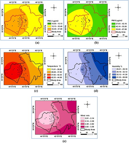
Generally, the obtained statistical values of PM_2.5 varied between 10 and 47.99 µg/m³ in the entire region. More specifically in the study area, the values of PM_2.5 ranged between 10 and12.13 µg/m³ (good air quality in green) covering a small part of the area, 12.13-35.49 µg/m³ (moderate in yellow) with predominant coverage, and 35.49-47.99 µg/m³ (unhealthy air for sensitive people in orange). On the other hand, PM₁₀ statistic values were calculated from 27.65-67.99 µg/m3 in the whole region, mostly representing good quality with values less than 55 µg/m³ (in green). The temperatures approximately raised from 11 to 45 °C from north-east to west, in the study area. In contrast, the percentage of humidity increased from 20 to 70 from west to east. Besides, wind speed values were calculated from 2 to 3.56 m/s with a slight increase from west to north-east, south, and south-east.

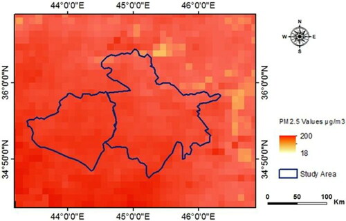
Based on the remotely sensed image, PM_2.5 values were mapped. The values ranged between 18-200 μg/m³ which approved the unhealthy air inside the study area during February 2020. Figure 5 represents the PM_2.5 distribution map based on the MODIS image.

Figure 5. The PM_2.5 distribution map based on the MODIS image.

4.2. Regression outputs

Table 2 represents the regression outputs of the July 2019 dataset, where most of the independent parameters exhibited a high level of correlation with PM_2.5. Table 3 represents the regression outputs of the February 2020 dataset.

Table 2. Regression outputs of July 2019 dataset.

Parameters	Intercept Coefficient	Parameters Coefficients	P-value	Standard Error
PM10	−25.6878	0.276	0.002228	0.082956
Temperature		1.405	2.52E-05	0.284294
Humidity		0.123	0.011793	0.046197
Wind		−5.563	0.000939	1.521399

Table 3. Regression outputs of February 2020 dataset.

Parameters	Intercept Coefficient	Parameters Coefficients	P-value	Standard Error
PM10	−124.074	1.754	0.002082	0.478542
Temperature		− 1.798	0.008828	0.603418
Humidity		1.016	0.000699	0.242964

To construct the model, the correlation was tested to measure the strength of the linear relationship between PM_2.5 and the other variables. All parameters showed a P-value lower than 0.05 indication the significant correlation with PM_2.5. However, in this step of the analysis, the main objective was to find the correlation between the parameters to influence the linear relationship.

For creating a regression model, it is essential to study the influential factors, with P-value < 0.05 as inputs, and preferably high values of R square. Based on equation 2(2) $$z_{\mathit{ijk}}=\mathrm{\mu }+t_{k\mathrm{ }}+{\beta }_{jk\mathrm{ }}+{\delta }_{\mathit{ijk}\mathrm{ }}$$(2) (multiple linear model equation), the regression was implemented. The case involved an analysis of the relationship between each independent parameter and the dependent variable PM_2.5. Under these conditions, we constructed the following equations from the regression outputs to predict PM_2.5 concentrations: (6) $${PM}_{2.5\left(\mathit{Estimated}\right)J\mathit{uly}\mathrm{ }2019}\mathrm{ }=-\mathrm{ }25.687+0.276\mathrm{*}{PM}_{10}+1.405\mathrm{*}T+0.123\mathrm{*}H-5.563\mathrm{*}W$$(6) $${PM}_{2.5\left(\mathit{Estimated}\right)F\mathit{ebruary}\mathrm{ }2020}\mathrm{ }=-124.074+1.754\mathrm{*}PM10\mathrm{ }-\mathrm{ }1.798T+\mathrm{ }1.016H\mathrm{ }\left(7\right)$$ where ${PM}_{2.5\mathrm{ }(\mathit{Estimated})}$ is the calculated particle matter concentration in µg/m³ with a diameter of 2.5 microns, PM₁₀ is particle matter concentration in µg/m³ with a diameter of 10 microns,$\mathrm{ }T$ in °C is the surface air temperature, $H$ % is the humidity of the environment, and $W$ m/s is the wind velocity. It is required to detect the possible reliance of the predictors for model condition construction. The predicted model is also beneficial for PM_2.5 estimations in non-monitored locations (Thongthammachart and Jinsart 2020).

The prediction equation was applied on a small subset of Kirkuk Province for some randomly selected points again. The estimation accuracy was achieved by a high value of R² (0.96) for July 2019 dataset. Also, the model was constructed based on 20 points collected in February 2020 by air quality multimeter device. The estimated accuracy was equal to (0.98) R². Afterward, model test validation was performed using additional values of PM_2.5. Moreover, Figure 6a represents a prediction map of PM_2.5 in Kirkuk and Sulaymaniyah provinces north of Iraq of July 2019, Figure 6b represents a prediction map of PM_2.5 in Kirkuk at an area of 5.6 km² of July 2019, and Figure 6c represents a prediction map of PM_2.5 in Kirkuk at an area of 5.6 km² of February 2020.

Figure 6. (a) Prediction map of PM_2.5 in Kirkuk and Sulaymaniyah provinces of July 2019. (b) Prediction map in Kirkuk at an area of 5.6 km² of July 2019. (c) Prediction map in Kirkuk at an area of 5.6 km² of February 2020.

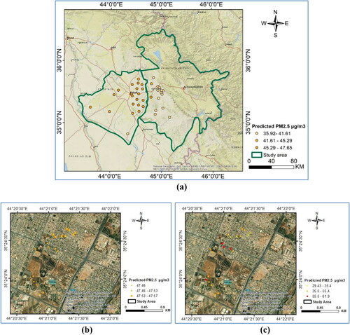
It is important to know that the estimated model did not achieve the real or the absolute prediction but it could be considered as the near value to the real (Shareef et al. 2014; Jumaah et al. 2019). The predicted PM_2.5 values ranged between 35.92 and 47.65 µg/m³ indicating unhealthy air quality for the sensitive groups in the two provinces north of Iraq during July 2019. The estimated values of PM_2.5 in the small subset area inside Kirkuk during July 2019 are ranged between 47.46-47.57 µg/m³. While February 2020 prediction map in the small subset area inside Kirkuk showed high values of PM_2.5 ranged between 29.43- 61.9 indicating three types of air quality; moderate (in yellow), unhealthy for the sensitive groups (in orange), and unhealthy (in red).

4.3. Cross-validation outputs

Validation was performed with the model-building in the study area; it means that the estimated PM_2.5 values were fit against the measured (ground truth) PM_2.5 values (Figure 7) PM_2.5 cross-validation.

Figure 7. PM2.5 cross-validation, (a) Predication validation at 5.6 km2 of July 2019, (b) Predication validation north of Iraq of July 2019, (c) Predication validation at 5.6 km2 of February 2020.

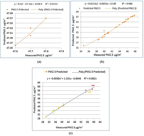
The correlation coefficient was calculated to evaluate the potential of prediction in the regression model. The results showed that all the parameters within the model equation correlated statistically, which indicated that the predictions made from the model were in good agreement with the inputs. As a result, the regression model generated a high correlation coefficient with an R² value of 0.98 in Kirkuk and Sulaymaniyah provinces. Furthermore, a high correlation coefficient with an R² value of 0.97 was acquired by the validation process of the same equation that was used to estimate PM_2.5 inside Kirkuk Province within the area of 5.6 km² based on the July 2019 dataset. Also, a high correlation coefficient with an R² value of 0.98 in Kirkuk at 5.6 km² was acquired by the validation process of the February 2020 dataset collected by the device. Moreover, the model validation was performed to fit the predicted PM_2.5 against the measured PM_2.5 data as tested. Figure 8 represents model validation in Kirkuk at 5.6 km².

Figure 8. Model-validation in Kirkuk at 5.6 km² of; (a) July 2019 (b) February 2020.

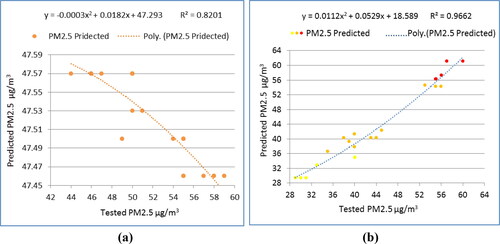
The obtained correlation coefficient R² was equal to 0.82 and 0.96 of July 2019 and February 2020 respectively. To compare with previous predictions in the north of Iraq, the lower correlation coefficient value might be due to PM_2.5 values variation during measurements, which refer to the average PM_2.5 value at each point. However, they describe the model ability in predicting by 82% and 96%.

5. Discussion

The concentration of PM_2.5 in Figure 4 depicted unhealthy air for sensitive people in the entire Kirkuk and west part of Sulaymaniyah province. However, by passing from the west borderline of Sulaymaniyah province, it was observed that the presence of PM_2.5 was at a moderate level in the north, south, east, and center of this province. The prediction of PM_2.5 using the regression method (Figure 6) indicated unhealthy air quality for the sensitive groups in the center borderline of the two provinces in July 2019. While the risk increased in Kirkuk during February 2020. Some locations appeared unhealthy air quality south of Kirkuk province. Besides the mapped PM_2.5 distribution of the study area in February showed the unhealthy air quality in the two provinces. The increment in air pollution (PM_2.5) lately in Sulaymaniyah related to unhampered industrial development which resulted in poor air quality (Arif et al. 2018) causing serious health problems . Based on blood disease maps during 2017, the detected increase in patients was determined in southern areas of Kirkuk city with minor distribution to blood disease patients in the city center and northern parts. In general, the disease conditioning factors were the reason for the disease occurrences in the study area (Ajaj et al. 2018). The economic and industrial growth that took in Sulaymaniyah city made poor air quality associated with crucial health problems, leading to an increase in the risk of death from cardiopulmonary diseases and lung cancer, specifically when people are exposed to high levels of pollutants over time (Arif et al. 2018). The roads and transportation sector were the most important sources of the PM_2.5 concentrations (Al-Arkawazi 2020) and long-term exposure to fine particles leads to respiration problems (Attiya and Jones 2020).

The health impact of PM₁₀ was determined as good and moderate air quality. Based on the results of PM₁₀ and its distribution, exposing zones to higher PM_2.5 with unhealthy air quality (the entire of Kirkuk and west part of Sulaymaniyah province) was classified as moderate AQI in terms of the presence of PM₁₀. The rest of the region was qualified as good AQI, regarding PM₁₀. Thus, there was no critical impact on human health in the study area in terms of PM₁₀ existents.

According to the IDW outputs of meteorological variables, Kirkuk province represented higher temperatures (42.55-44.99 °C), lower humidity (20.01-32.12%) with lower wind speed (2.01-2.39 m/s) to compare with Sulaymaniyah province. The concentration of PM_2.5 showed a correlation with those factors and they might contribute to the air quality and pollution in Kirkuk.

Also, according to the proposed model, it indicated a high correlation between the PM_2.5 variable and the independent factors. So, in order to test each parameter and its contribution, we investigated the relationship between PM_2.5 and each parameter. It revealed that the temperature was the most important independent variable and it highly contributed to the assessment, followed by PM₁₀, wind, and humidity. In Figure 7 the cross-validation applied for the model to gain the typical precision and to examine the range of equivalent at the recorded positions. The results showed the full recorded datasets were in the confidence boundary with an R² value of 0.98 in the north of Iraq (in the two provinces) and an R² value of 0.97 and 0.98 in the small subset, inside Kirkuk for July 2019 and February 2020 respectively. As it is shown in Figure 8, using the ground truths, the degree of confidence with observations was adopted, besides, to test the performance of the model. The result indicated that the predicted values were verified with R² equal to 0.82 and 0.96 for July 2019 and February 2020 respectively.

6. Conclusion

To calculate the ground-level PM_2.5 concentrations by a polynomial model, this paper studied the correlation of PM₁₀ in addition to significant meteorological parameters such as humidity, air surface temperature, and wind speed as the independent variables. Two equations to estimate PM_2.5 concentrations were developed and evaluated based on July 2019 and February 2020 datasets. The results showed that the use of all meteorological datasets could significantly improve the model performance in the region. Additionally, our finding indicated that PM₁₀ had also a significant relationship with PM_2.5 prediction.

Furthermore, the prediction was at high accuracy with R² = 0.98. Accuracy assessment also was done in a small subset in Kirkuk using some measured samples as ground truth data. Upon chosen points, results displayed a high accuracy with R² = 0.97 and 0.98 of July 2019 and February 2020 respectively. The result of the model cross-validation with R² evaluated the model by R² = 0.82 and 0.96 of July 2019 and February 2020 respectively. Furthermore, the implications of the health impacts of PM_2.5 prediction and its distribution in the two provinces were within moderate to unhealthy air quality for people with respiratory diseases, and the sensitive people are advised to limit outdoor exertion. Besides the unhealthy increased air quality in 2020.

The research highlighted the effect of industrial zones and recommended monitoring, control, and reducing particles and pollutants exposures from factories using alternative methods and mitigation strategies. By promoting clean and renewable energies instead of fossil fuel, increasing people's awareness to deal with the impact of pollutants, increasing afforestation around the cities to reduce the effects of pollution along with early warning and prediction, the future would be more promising. To improve public health, and for a more and broad understanding of the relationship between compounds of PM_2.5 and PM₁₀ with their toxicological impacts, further investigations on sampling sites and causes of air contamination should be made in the study area. Moreover, our method could brighten the study of epidemiology and recent COVID-19 pandemic in terms of PM concentrations and spatial distribution of infections. Future work will be based on other influential factors in exceeding PM concentrations and their spatial distribution in the region incorporation with more meteorological parameters.

Acknowledgment

The authors would like to thank the team who has helped in carrying out the field measurements to introduce this research.

Disclosure statement

No potential conflict of interest was reported by the authors.

Data availability statement

The data that support the findings of this study are available from the corresponding author, Bahareh Kalantar, upon reasonable request.

Additional information

Funding

The authors would like to thank the RIKEN Centre for Advanced Intelligence Project (AIP), Japan for the APC funding.

References

- Adams K, Greenbaum DS, Shaikh R, van Erp AM, Russell AG. 2015. Particulate matter components, sources, and health: Systematic approaches to testing effects. J Air Waste Manage Assoc. 65(5):544–558.
- Ajaj QM, Pradhan B, Noori AM, Jebur MN. 2017. Spatial monitoring of desertification extent in western Iraq using Landsat images and GIS. Land Degrad Develop. 28(8):2418–2431.
- Ajaj QM, Shareef MA, Hassan ND, Noori AM, Hasan SF. 2018. GIS-based spatial modeling to mapping and estimation relative risk of different diseases using inverse distance weighting (IDW) interpolation algorithm and evidential belief function (EBF)(Case study: Minor Part of Kirkuk City, Iraq). Int J Eng Technol. 7(4.37):185–191. https://www.researchgate.net/publication/329702527.
- Al-Arkawazi SAF. 2020. Studying the relation between the engine size and manufacturing year of gasoline-fueled vehicles and exhaust emission percentages and concentrations. J Mater Environ Sci. 11(2):196–219.
- Al-Bayati RM, Al-Salihi AM. 2019. Monitoring carbon dioxide from (AIRS) over Iraq during 2003–2016. In: AIP Conference Proceedings. Vol. 2144. AIP Publishing; p. 030007.
- Ali JJM, Nori IM, Hama SJ, Rashed SO. 2015. Water harvesting through utilization of wild almond as rootstocks for production of peach, apricot and plum under dry land farming in Sulaymaniyah region. Int J Innovative Sci Eng Technol. 2(8): 705–724. http://ijiset.com/vol2/v2s8/IJISET_V2_I8_92.pdf.
- Anenberg SC, Miller J, Henze DK, Minjares R, Achakulwisut P. 2019. The global burden of transportation tailpipe emissions on air pollution-related mortality in 2010 and 2015. Environ Res Lett. 14(9):094012.
- Arif AT, Maschowski C, Khanaqa P, Garra P, Garcia-Käufer M, Wingert N, Mersch-Sundermann V, Gminski R, Trouvé G, Gieré R. 2018. Characterization and in vitro biological effects of ambient air PM10 from a rural, an industrial and an urban site in Sulaimani City, Iraq. Toxicol Environ Chem. 100(4):373–394.
- Attiya AA, Jones BG. 2020. Climatology of Iraqi dust events during 1980–2015. SN Appl Sci. 2(5):1–16.
- Bali S. 2020. Indian air quality prediction and analysis using machine learning. J Eng Sci. 11(5): 554–557.
- Boldo E, Medina S, Le Tertre A, Hurley F, Mücke HG, Ballester F, Aguilera I. 2006. Apheis: Health impact assessment of long-term exposure to PM 2.5 in 23 European cities. Eur J Epidemiol. 21(6):449–458.
- Borrego C, Costa AM, Ginja J, Amorim M, Coutinho M, Karatzas K, Sioumis T, Katsifarakis N, Konstantinidis K, De Vito S, et al. 2016. Assessment of air quality microsensors versus reference methods: the EuNetAir joint exercise. Atmos Environ. 147:246–263.
- Buraihi FH, Shariff ARM. 2015. Selection of rainwater harvesting sites by using remote sensing and GIS techniques: a case study of Kirkuk, Iraq. Jurnal Teknologi. 76(15): 75–81.
- Chambliss SE, Silva R, West JJ, Zeinali M, Minjares R. 2014. Estimating source-attributable health impacts of ambient fine particulate matter exposure: global premature mortality from surface transportation emissions in 2005. Environ Res Lett. 9(10):104009.
- Chen L, Bai Z, Kong S, Han B, You Y, Ding X, Du S, Liu A. 2010. A land use regression for predicting NO2 and PM10 concentrations in different seasons in Tianjin region, China. J Environ Sci. 22(9):1364–1373.
- Cressie N. 1992. Statistics for spatial data. Terra Nova. 4(5):613–617.
- Crippa M, Janssens-Maenhout G, Guizzardi D, Dingenen RV, Dentener F. 2019. Contribution and uncertainty of sectorial and regional emissions to regional and global PM 2.5 health impacts. Atmos Chem Phys. 19(7):5165–5186.
- David LM, Ravishankara AR, Kodros JK, Pierce JR, Venkataraman C, Sadavarte P. 2019. Premature mortality due to PM2.5 over India: effect of atmospheric transport and anthropogenic emissions. Geohealth. 3(1):2–10.
- Donnelly A, Misstear B, Broderick B. 2019. Air quality modelling for Ireland. EPA Research Report. Ireland: Environmental Protection Agency. https://arrow.dit.ie/engschcivrep/13.
- Fan M, He G, Zhou M. 2020. The winter choke: Coal-Fired heating, air pollution, and mortality in China. J Health Econ. 71:102316.
- Fathoni U, Zakaria CM, Rohayu CO. 2013. Development of corrosion risk map for Peninsular Malaysia using climatic and air pollution data. In IOP Conference Series: Earth and Environmental Science. Vol. 16. IOP Publishing; p. 012088.
- Ganesh SS, Arulmozhivarman P, Tatavarti VR. 2018. Prediction of PM 2.5 using an ensemble of artificial neural networks and regression models. J Ambient Intell Hum Comput.:1–11.doi: https://doi.org/10.1007/s12652-018-0801-8
- Gelfand AE, Diggle P, Guttorp P, Fuentes M. 2010. Handbook of spatial statistics. 1st ed. Boca Raton, FL: CRC Press.
- Gong G, Mattevada S, O’Bryant SE. 2014. Comparison of the accuracy of kriging and IDW interpolations in estimating groundwater arsenic concentrations in Texas. Environ Res. 130:59–69.
- Gui K, Che H, Zeng Z, Wang Y, Zhai S, Wang Z, Luo M, Zhang L, Liao T, Zhao H, et al. 2020. Construction of a virtual PM2.5 observation network in China based on high-density surface meteorological observations using the extreme gradient boosting model. Environ Int. 141:105801.
- Hayes RB, Lim C, Zhang Y, Cromar K, Shao Y, Reynolds HR, Silverman DT, Jones RR, Park Y, Jerrett M, et al. 2020. PM2. 5 air pollution and cause-specific cardiovascular disease mortality. Int J Epidemiol. 49(1):25–35.
- He K, Yang F, Ma Y, Zhang Q, Yao X, Chan CK, Cadle S, Chan T, Mulawa P. 2001. The characteristics of PM2.5 in Beijing, China. Atmos Environ. 35(29):4959–4970.
- Hu X, Waller LA, Al-Hamdan MZ, Crosson WL, Estes MG, Estes SM, Quattrochi DA, Sarnat JA, Liu Y. 2013. Estimating ground-level PM(2.5) concentrations in the southeastern U.S. using geographically weighted regression. Environ Res. 121:1–10.
- Hvidtfeldt UA, Ketzel M, Sørensen M, Hertel O, Khan J, Brandt J, Raaschou-Nielsen O. 2018. Evaluation of the Danish AirGIS air pollution modeling system against measured concentrations of PM2. 5, PM10, and black carbon. Environ Epidemiol. 2(2):e014.
- Ito K, Christensen WF, Eatough DJ, Henry RC, Kim E, Laden F, Lall R, Larson TV, Neas L, Hopke PK, et al. 2006. PM source apportionment and health effects: 2. An investigation of intermethod variability in associations between source-apportioned fine particle mass and daily mortality in Washington, DC. J Expo Sci Environ Epidemiol. 16(4):300–310.
- Jassim MS, Coskuner G. 2017. Assessment of spatial variations of particulate matter (PM 10 and PM 2.5) in Bahrain identified by air quality index (AQI). Arab J Geosci. 10(1):19.
- Jumaah HJ, Ameen MH, Kalantar B, Rizeei HM, Jumaah SJ. 2019. Air quality index prediction using IDW geostatistical technique and OLS-based GIS technique in Kuala Lumpur, Malaysia. Geomatics Nat Hazards Risk. 10(1):2185–2199.
- Jumaah HJ, Mansor S, Pradhan B, Adam SN. 2018. UAV-based PM2. 5 monitoring for small-scale urban areas. Int J Geoinformatics. 14(4): 61–69. https://www.researchgate.net/publication/333378629_UAVbasedPM25monitoring_forsmall-scaleurbanareas.
- Kong L, Tian G. 2020. Assessment of the Spatio-temporal pattern of PM 2.5 and its driving factors using a land-use regression model in Beijing, China. Environ Monit Assess. 192(2):95.
- Li C, Huang Y, Guo H, Wu G, Wang Y, Li W, Cui L. 2019. The concentrations and removal effects of PM10 and PM2. 5 on a Wetland in Beijing. Sustainability. 11(5):1312.
- Liu CM. 2002. Effect of PM2. 5 on AQI in Taiwan. Environ Modell Software. 17(1):29–37.
- Manikonda A, Zíková N, Hopke PK, Ferro AR. 2016. Laboratory assessment of low-cost PM monitors. J Aerosol Sci. 102:29–40.
- Marcazzan GM, Vaccaro S, Valli G, Vecchi R. 2001. Characterization of PM10 and PM2.5 particulate matter in the ambient air of Milan (Italy). Atmos Environ. 35(27):4639–4650. (01)00124-8
- Mohamedali SA, Ameen MH, Saeb A. 2020. Repercussion of petroleum industry and vehicle emissions on Kirkuk air quality using GIS. 10th International Conference on Research in Engineering, Science, and Technology; Feb 21–23; Rome, Italy.
- Zaki MMF, Mohamad Ismail MA, Govindasamy D, Zainal Abidin MH. 2019. Interpretation and development of top-surface grid in subsurface ground profile using Inverse Distance Weighting (IDW) method for twin tunnel project in Kenny Hill Formation. BGSM. 67:91–97.
- Nazif A, Mohammed NI, Malakahmad A, Abualqumboz MS. 2016. Application of step wise regression analysis in predicting future particulate matter concentration episode. Water Air Soil Pollut. 227(4):117.
- Querol X, Alastuey A, Ruiz CR, Artiñano B, Hansson HC, Harrison RM, Buringh E, ten Brink HM, Lutz M, Bruckmann P, et al. 2004. Speciation and origin of PM10 and PM2. 5 in selected European cities. Atmos Environ. 38(38):6547–6555.
- Sahu SP, Patra AK. 2020. Development and assessment of multiple regression and neural network models for prediction of respirable PM in the vicinity of a surface coal mine in India. Arab J Geosci. 13(17):1–16.
- Saxena P, Jagdeesh MK. 2019. Similarity indexing & GIS analysis of air pollution. arXiv preprint arXiv:1906.08756. https://arxiv.org/abs/1906.08756v1.
- Setianto A, Triandini T. 2015. Comparison of kriging and inverse distance weighted (IDW) interpolation methods in lineament extraction and analysis. J Appl Geol. 5(1): 21–29.
- Shareef MA, Toumi A, Khenchaf A. 2014. Prediction of water quality parameters from SAR images by using multivariate and texture analysis models. In: SAR Image Analysis, Modeling, and Techniques XIV. Vol. 9243. International Society for Optics and Photonics; p. 924319.
- Silva RA, Adelman Z, Fry MM, West JJ. 2016. The impact of individual anthropogenic emissions sectors on the global burden of human mortality due to ambient air pollution. Environ Health Perspect. 124(11):1776–1784.
- Skidmore A, ed. 2017. Environmental modeling with GIS and remote sensing. CRC Press, London, New York .
- Sun L, Wei Y, Cai H, Yan J, Xiao J. 2019. Improved fast adaptive IDW interpolation algorithm based on the borehole data sample characteristic and its application. J Phys: Conf Ser. 1284(1):012074.
- Thongthammachart T, Jinsart W. 2020. Estimating PM2. 5 concentrations with statistical distribution techniques for health risk assessment in Bangkok. Hum Ecol Risk Assess: Int J. 26(7):1848–1816.
- Tian J, Chen D. 2010. A semi-empirical model for predicting hourly ground-level fine particulate matter (PM2. 5) concentration in southern Ontario from satellite remote sensing and ground-based meteorological measurements. Remote Sens Environ. 114(2):221–229.
- Tuna F, Buluc M. 2015. Analysis of PM10 pollutant in Istanbul by using Kriging and IDW methods: between 2003 and 2012. Int J Comput Inf Technol. 4(1):170–175.
- Ul-Saufie AZ, Yahaya AS, Ramli NA, Rosaida N, Hamid HA. 2013. Future daily PM10 concentrations prediction by combining regression models and feedforward backpropagation models with principle component analysis (PCA). Atmos Environ. 77:621–630.
- Van Donkelaar A, Martin RV, Park RJ. 2006. Estimating ground‐level PM2. 5 using aerosol optical depth determined from satellite remote sensing. J Geophys Res. 111(D21): 1–10.
- Vorapracha P, Phonprasert P, Khanaruksombat S, Pijarn N. 2015. A comparison of spatial interpolation methods for predicting concentrations of particle pollution (PM10). Int J Chem Environ Biol Sci. 3(4):302–306.
- Wang YC, Chen GW. 2017. Efficient data gathering and estimation for metropolitan air quality monitoring by using vehicular sensor networks. IEEE Trans Veh Technol. 66(8):7234–7248.
- Wu M, Huang J, Liu N, Ma R, Wang Y, Zhang L. 2018. A hybrid air pollution reconstruction by adaptive interpolation method. In: Proceedings of the 16th ACM Conference on Embedded Networked Sensor Systems; p. 408–409.
- Yang Y, Zheng Z, Bian K, Song L, Han Z. 2018. Real-time profiling of fine-grained air quality index distribution using UAV sensing. IEEE Internet Things J. 5(1):186–198.
- Zeinalnezhad M, Chofreh AG, Goni FA, Klemeš JJ. 2020. Air pollution prediction using semi-experimental regression model and adaptive neuro-fuzzy inference system. J Cleaner Prod. 261:121218.