Landslide susceptibility mapping by attentional factorization machines considering feature interactions

Abstract

Landslide susceptibility mapping (LSM) is a commonly used approach to reduce landslide risk. However, conventional LSM methods generally only consider the influence of each single conditioning factor on landslide occurrence or absence, which neglects the interactions of different conditioning factors and may lead to biased LSM results. Therefore, this study aims to use a new machine learning model—attentional factorization machines (AFM)—to explicitly consider the influence of feature interactions in LSM to improve and obtain more reliable LSM results. The Anhua County in China is chosen as the study area. The area under the receiver operating characteristic curve (AUC) and statistical indicators are used to evaluate the performance of LSM models. For comparison, the common LSM models such as the logistic regression (LR) and random forest (RF) models are also used to conduct the LSM. The results show that the performance of AFM is a little better than RF in the AUC metric, whereas the LR model has the worst performance. Compared with general LSM models, AFM considers feature interactions by introducing an attention mechanism to learn the weight of different feature combinations, which not only ensures the model interpretability but also improves the model performance.

Keywords:

• Landslide susceptibility mapping
• machine learning
• random forest
• feature interaction
• attentional factorization machine (AFM).

1. Introduction

Landslide is one of the most widespread geological hazards worldwide and has obvious consequences and impacts on economics and human welfare (Pham et al. 2020). In terms of economic losses alone, it is estimated that the annual losses caused by landslides are about 1.62 billion US dollars in the United States, 1.96 million US dollars in Nepal, and 2.37 billion US dollars in China (Bai et al. 2012). To reduce landslide risk, many governments and research institutions have devoted themselves to studying landslide susceptibility since the 1970s and 1980s (Reichenbach et al. 2018).

Landslide susceptibility is the possibility of landslide occurrence in a given region based on the local environmental conditions (Aleotti and Chowdhury 1999). It is assessed based on the assumption that future landslides will take place under similar environmental conditions where past landslides occurred (Guzzetti et al. 1999). With this assumption in mind, landslide susceptibility mapping (LSM) aims to find out what factors can represent environmental conditions and to obtain the relationship between the factors and landslides. It is concluded from the literature that the conditioning factors that usually control landslides occurrence or absence include topography, geology, geotechnical properties, vegetation factors (Reichenbach et al. 2018). The relationships between the factors and landslides are explained in two ways: qualitative and quantitative. Qualitative methods are based on expert knowledge. For example, geomorphological LSM is a qualitative method that is directly carried out in the field based on the experience of investigators in estimating the actual and potential slope failures (Aleotti and Chowdhury 1999).

By contrast, quantitative methods conduct LSM according to the numerical expression between the conditioning factors and landslides (Dehnavi et al. 2015), which can also be divided into two main categories: geotechnical methods and statistical methods. Geotechnical methods are based on slope stability theory and principles such as infinite slope, limit equilibrium, and finite element methods (Reichenbach et al. 2018). Although geotechnical methods can accurately determine the stability of a specific landslide based on mechanics, they need a mass of accurate hydrological and geotechnical mechanical parameters as inputs, and these properties are assumed to be homogeneous over the area. As such, geotechnical methods can only be applicable to study areas with a relatively small size (Wang et al. 2019). In contrast to geotechnical methods, the data used by statistical methods are easier to obtain and they can be applied to a larger area (Reichenbach et al. 2018). In recent years, there has been increasing popularity in using statistical methods for LSM (Juliev et al. 2019; Wang et al. 2020), which has greatly facilitated the development and application of LSM. The most popular statistical methods are machine learning methods, including but not limited to support vector machine (Sameen et al. 2020), random forest (RF) (Dou et al. 2019), adaptive neuro-fuzzy inference system (Lee et al. 2015), and artificial neural networks (Zhang et al. 2021).

However, to our best knowledge, the available general statistical methods and machine learning methods only consider the influence of a single conditioning factor in LSM (Merghadi et al. 2020), which neglects the effect of feature interactions. In fact, the effect of the interaction of two factors may be greater than that of a single factor. For example, compared to the effect of sparse vegetation alone, a combination of sparse vegetation and heavy rainfall is more likely to lead to landslides. Hence, it is necessary to take the interaction of different factors into account in LSM. Yet, considering feature interactions in LSM has been limited.

To address the above problem, this paper proposes using the attentional factorization machines (AFM) (Xiao et al. 2017), which is the adaption of the factorization machines (FMs) (Rendle 2011) by introducing the attention mechanism, to conduct LSM with considering feature interactions. To the best of our knowledge, most LSM models used in previous studies, such as RF and logistic regression (LR), only consider first-order features, whereas AFM considers the second-order features as well as the first-order features, which strengthens the nonlinear expression of the model. AFM can provide different weights for different combinations of factors (i.e. feature interactions), which indeed represents the effect of feature interactions on the underlying model. Additionally, AFM has been applied in other fields such as recommendation systems (Tang et al. 2020) for dealing with problems of feature interactions, but is rarely seen in the application of LSM. Therefore, the main purposes of the study are to explore the feasibility of the proposed method for LSM and illustrate the importance of feature interactions on LSM. Another is to compare the performance of the proposed method with traditional machine learning methods to obtain a more reliable LSM result. For illustration, Anhua County located in the central Hunan Province of China, which is a landslide-prone area but was rarely studied before, is selected as the study area. Two LSM methods, RF and LR, which have been frequently applied in landslide prediction modelling (Wang et al. 2015; Chen et al. 2017), are adopted as representative traditional machine learning methods to model the landslide susceptibility of the study area for comparison.

2. Materials

2.1. Study area

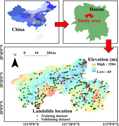
Anhua County is in the central area of the Hunan Province of China. It is distributed between the altitudes of 27°58′54″ N and 28°38′37″ N and longitudes of 110°43′07″ E and 111°58′51″ E, as shown in Figure 1. The county has an area of about 4950 km², which contains 163 streams. The county has a subtropical seasonal monsoon climate with four distinct seasons and abundant rainfall. According to meteorological data from 1963 to 2012 (50 years), the annual average temperature is about 16.4 °C, while the average temperature in July and January is 27.5 °C and 4.6 °C, respectively. Meanwhile, the area is one of the four major rainstorm centres in Hunan Province. The average annual precipitation is 1738 mm, and the annual average number of precipitation days is 170.86 mm. The county is located at the hinterland of the Xuefeng Mountains, which pertains to a medium and low mountain landform. Within the territory of the county, the mountains stand tall and the terrain is strongly cut with very developed V-shaped valleys as well as steep slopes. Besides, from the census of 2013, over one million people are living in the area, implying many human engineering activities there. As such, the county is a landslide-prone area. During the years from 2015 to 2018, about 8,260 people were affected by the landslides in the study area, with two deaths and a direct economic loss of about 121.452 million yuan.

Figure 1. Location of the study area and landslide inventory map.

2.2. Landslide inventory

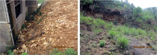
Based on the assumption that future landslides will take place under the environmental conditions where past landslides occurred (Guzzetti et al. 1999), it is important to obtain an accurate landslide inventory map for statistical LSM. Landslide inventory can be prepared in various ways, such as field surveys and satellite image recognition (Sara et al. 2015; Chen et al. 2017). In this study, 434 landslides are obtained through field surveys and referring to the historical materials of the Geological Disaster Emergency Center of Hunan Province, as schematically shown in Figure 1. In general, it is seen from the figure that the landslides are distributed all over the study area. They are characterized by large amounts, small scales, and wide distributions. Statistics show that the landslide volume ranges from 8 m³ to 1.5 × 10⁵ m³, and soil and gravel soil landslide are the main landslides that account for the majority of these recorded landslides (Figure 2). These landslides are mainly activated by seasonal heavy rainfall and frequent human engineering activities (e.g. cutting slopes for buildings and roads, changes in vegetation). Considering the common process for LSM, these landslide samples are randomly divided into two parts: 304 (70%) samples out of them are used for training and the remaining 130 (30%) samples are retained for the validation of the calibrated susceptibility models (Dou et al. 2019; Wang et al. 2020). Note that such ratio of training and validating data has been widely used in the literature (Pham et al. 2019; Hu et al. 2020; Zhao and Chen 2020; Dou et al. 2020b) and some internal analyses also found this ratio yield good results.

Figure 2. Typical landslide pictures in Anhua County.

2.3. Landslide-related conditioning factors

Landslide conditioning factors are factors controlling landslide occurrence or absence. The selection of landslide conditioning factors is therefore important for LSM. In the literature, landslide conditioning factors are often selected based on the geomorphological characteristics of the study area, types of landslides, and methods used (Hung et al. 2016). In this study, fifteen conditioning factors, including elevation, slope degree, slope aspect, slope position, micro-geomorphology, plan curvature, profile curvature, topographic wetness index (TWI), lithology, distance to fault, distance to road and distance to river, normalized difference vegetation index (NDVI), land use and annual rainfall, are initially selected, which are later analyzed through multicollinearity analysis. These factors are supposed to be directly or indirectly linked to the stability of the slopes in the study area. The fifteen conditioning factors are mainly obtained from the data sources such as field investigation and free remote sensing images. For convenience, the sources for different factors are tabulated in Table 1. It is seen from the table that the elevation, slope degree, slope aspect, slope position, micro-geomorphology, plan curvature, profile curvature, TWI are obtained from the Digital Elevation Model (DEM) (Hung et al. 2016). The 1:250,000 geological map (http://zrzyt.hunan.gov.cn/) is used to extract the lithology and distance to fault, while the distance to road and distance to river are obtained from the 1:250,000 topographic map (http://zrzyt.hunan.gov.cn/). Meanwhile, the Landsat 8 OLI image is used to produce the NDVI. Furthermore, the annual rainfall and land use data are obtained from the land use map and rainfall map (www.gscloud.cn), respectively, both with a resolution of 30 m.

Table 1. Sources of landslide conditioning factors.

Sources	Factors
ASTER DEM (30 m)	Elevation, slope degree, slope aspect, slope position, micro-geomorphology, plan curvature, profile curvature, TWI
1:250,000 geological map	Lithology, distance to fault
1:250,000 topographic map	Distance to road, distance to river
Landsat 8 OLI (30 m)	NDVI
Land use map (30 m)	Land use
Rainfall map (30 m)	Annual rainfall

It should be noted that the fifteen factors are either continuous or discrete variables. For continuous variables, they are all converted to discrete variables (Huang et al. 2020; Yi et al. 2020), but there is no uniform standard for ascertaining the number of attribute intervals. When the number of attribute intervals is small, the division of continuous variables will be rough. By contrast, when the number of attribute intervals is large, the computational expense will be high, and the modelling process will become complex. In the literature, the number of attribute intervals is usually set to 4, 8, or 12 (Dehnavi et al. 2015; Chen and Chen 2021). According to Huang et al. (2020), an attribute interval number of 8 is commonly suitable for LSM. Hence, the continuous variables in this study are divided into 8 classes. Note that all factors are processed in ArcGIS software and converted to a grid cell with a resolution of 30 m, as shown in Figure 3. The description of each factor is summarized in Table 2 and presented as follows.

Figure 3. Spatial database for LSM: (a) slope degree; (b) slope aspect; (c) plan curvature; (d) profile curvature; (e) micro-geomorphology; (f) slope position; (g) TWI; (h) lithology; (i) distance to fault; (j) distance to road; (k) distance to river; (l) NDVI; (m) land use; (n) annual rainfall.

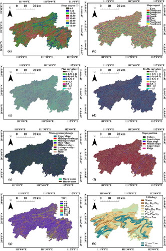
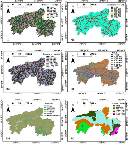
Table 2. Landside conditioning factors and their classes.

Conditioning factors	Classes	Data scale
Elevation (m)	<136; 136–249; 249–366; 366–489; 489–631; 631–821; 821–1078; >1078	Continuous
Slope degree (°)	<5; 5–10; 10–20; 20–30; 30–40; 40–50; 50–60; >60	Continuous
Slope aspect (°)	F (−1); N (0–22.5; 337.5–360); NE (22.5–67.5); E (67.5–112.5); SE (112.5–157.5); S (157.5–202.5); SW (202.5–247.5); W (247.5–292.5); NW (292.5–337.5)	Continuous
Plan curvature (m/100)	< −1.5; (−1.5)–(−1); (−1)–(−0.5); −0.5–0; 0–0.5; 0.5–1; 1–1.5; >1.5	Continuous
Profile curvature (m/100)	−1.5<; (−1.5)–(−1); (−1)–(−0.5); −0.5–0; 0–0.5; 0.5–1; 1–1.5; >1.5	Continuous
Micro-geomorphology	1; 2; 3; 4; 5; 6; 7; 8; 9; 10	Categorical
Slope position	Ridge; upper slope; middle slope; flats slope; lower slopes; valleys	Categorical
TWI	<4; 4–6; 6–8; 8–10; 10–12; 12–14; 14–20; >20	Continuous
Lithology	1; 2; 3; 4; 5; 6; 7; 8	Categorical
Distance to fault (m)	<200; 200–400; 400–600; 600–800; 800–1000; 1000–1200; 1200–1400; >1400	Continuous
Distance to road (m)	<100; 100–200; 200–300; 300–400; 400–500; 500–600; 600–700; >700	Continuous
Distance to river (m)	<200; 200–400; 400–600; 600–800; 800–1000; 1000–1200; 1200–1400; >1400	Continuous
NDVI	<0.01; 0.01–0.07; 0.07–0.11; 0.11–0.15; 0.15–0.19; 0.19–0.23; 0.23–0.27; >0.27	Continuous
Land use	Water; grassland; plowland; wetland; forest; artificial surface	Categorical
Annual rainfall (mm)	<900; 900–980; 980–1060; 1060–1140; 1140–1220; 1220–1300; 1300–1380; >1300	Continuous

The elevation varies from −65 to 1584 m, which is divided into 8 classes based on the natural break method, as shown in Figure 1. The slope degree ranges from 0° and 62° and is also classified into 8 classes (see Figure 3(a)). Figure 3(b) shows the map of slope aspect, which is related to the direction of precipitation, wind, and sunlight (Juliev et al. 2019). It is classified into nine categories: flat, north, northeast, east, southeast, south, southwest, west, and northwest. The plan curvature reflects the slope of the aspect, which describes the horizontal form of the topography. The profile curvature reflects the complexity of topography and can be determined as the slope of the slope. Both the plan curvature and profile curvature are continuous variables and are also divided into 8 classes, as shown in Figure 3(c, d).

Micro-geomorphology refers to the landform with relatively small scales, which will affect groundwater level, groundwater distribution, surface runoff, and vegetation type, thereby affecting the development of landslides. Weiss (2001) divided micro-geomorphology into 10 categories, but this study adopts 8 categories, as shown in Figure 3(e). Slope position refers to the geomorphic position of the slope surface. Many physical and biological processes acting on the landscape are highly correlated with slope position (Weiss 2001). The slope position of a grid unit is judged by using the difference between the elevation of the grid unit and the average elevation of a certain number of grid units around it, in combination with the slope degree of the grid unit. Slope position is divided into six groups: ridge, upper slope, middle slope, flats slope, lower slope, and valleys, as shown in Figure 3(f). Figure 3(g) shows the distribution of TWI in the study area, which represents the influence of topographic features on the spatial distribution of soil water. The moisture content and distribution in the soil will affect the soil and vegetation on the surface of slopes, and thus affecting landslide occurrence.

Geology plays a very important role in landslide susceptibility not only because of different lithological classes but also owing to the mechanical and hydraulic characteristics associated with them (Merghadi et al. 2020). This study area is divided into 8 categories based on lithology, as shown in Figure 3(h). Faults are directly related to regional tectonic activity and its feature is the presence of weak and fractured rocks (Pham et al. 2020). Figure 3(i) shows that distance to fault is divided into 8 classes with an interval of 200 m.

The factors of distance to road and distance to river are obtained from the topographic map. Distance to river reflects the influence of the hydrologic environment on landslides. Distance to road shows the influence of human engineering activities on the landslide environment. These two factors are divided into 8 equidistant classes with an interval of 200 m and 100 m, respectively, as shown in Figure 3(j, k).

NDVI index can provide a quantitative evaluation of regional vegetation cover. It can be formulated as (1) $$\mathrm{NDVI}=\frac{\mathit{Band}5-\mathit{Band}4}{\mathit{Band}5+\mathit{Band}4}$$(1) where Band5 and Band4 are the near-infrared and red bands in Landsat 8 OLI. Here, the NDVI map shown in Figure 3(l) is generated by satellite imagery (Landsat 8 OLI) on April 14, 2015.

Land use has been a predisposing factor for LSM in many studies (Juliev et al. 2019). Different land use types can affect the size, frequency, and types of landslides. It is also possible to change the initiation and acceleration thresholds of certain landslides (Pereira et al. 2020). The land use map is shown in Figure 3(m) indicates that there are mainly six land use types in the study area, including water, grassland, plowland, wetland, forest, and artificial surface.

Landslides are usually triggered by earthquakes and rainfall. In this study area, landslides triggered by rainfall are much more frequent than landslides triggered by earthquakes. The annual average rainfall reflects the distribution characteristics of average rainfall in the study area, which has a certain influence on the change of groundwater level and shear strengths of soil slopes (Chen et al. 2017). As most landslides in this region occurred during the flood season from March to August, the average rainfall during the flood season (hereafter referred to as the annual rainfall) is adopted as a landslide conditioning factor, as shown in Figure 3(n).

3. Methods

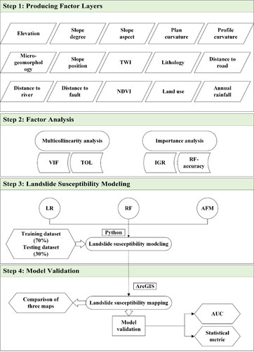
The entire workflow for this study is executed by following the flow chart in Figure 4, which mainly consists of four steps. Firstly, spatial data of landslide inventory and conditioning factors are prepared using ArcGIS software. Then, some statistical indices such as tolerance (TOL) and variance inflation factor (VIF) are used to analyze the multicollinearity and importance of the factors. Thereafter, the LSM models (i.e. LR, RF, and AFM) for the study area are respectively constructed. Finally, three landslide susceptibility maps are obtained and the performance of the three models is illustrated and compared based on the value of AUC and other metrics. Since the first step is described before, only the methods used in the remaining steps are described in the following subsections.

Figure 4. The framework of LSM in this study.

3.1. Multicollinearity analysis of conditioning factors

In LSM, checking the multicollinearity among different conditioning factors is an indispensable step. If there is a strong linear correlation among the aforementioned factors, it is considered that redundant factors exist in the original set of conditioning factors. The multicollinearity problem will lead to difficulty in landslide prediction and errored results (Chen and Chen 2021). There are two statistical parameters called TOL and VIF, which is a pair of reciprocals, for analyzing the multicollinearity problem. When TOL < 0.1 or VIF > 10, it means that there is serious multicollinearity (Dou et al. 2020a). For a specific landslide conditioning factor, TOL and VIF are calculated as follows: (2) $$\mathrm{VIF}=\frac{1}{1-R^2}$$(2) (3) $$\mathrm{TOL}=\frac{1}{\mathrm{VIF}}$$(3) where $R^2$ is the coefficient of determination of the regression between the factor of interest and the other landslide conditioning factors.

3.2. Importance of landslide-related conditioning factors

After multicollinearity analysis of the conditioning factors, a key step is to analyze the importance of the remaining conditioning factors and identify the most effective ones. The reason is that some unimportant factors in the dataset may produce noises and affect the model predictive capability. In this study, the information gain ratio (IGR) method (Dai and Xu 2013) is performed on the training dataset to obtain the importance of the input variables. The higher the IGR value of a landslide conditioning factor is, the greater the influence of the factor on the model will be. Factors with an IGR of 0 do not contribute to the model and should be removed before modelling.

3.3. Attentional factorization machines (AFM)

AFM is developed based on factorization machines (Rendle 2011). FM is a supervised learning approach that enhances linear regression models by incorporating second-order factor interactions as: (4) $${\widehat{y}}_{FM}\left(\mathit{X}\right)={\omega }_0+\sum _{i=1}^n{\omega }_i{x}_i+\sum _{i=1}^n\sum _{j=i+1}^n{\widehat{\omega }}_{ij}{x}_i{x}_j$$(4) where ${\omega }_0$ denotes the global bias; ${\omega }_i$ is the weight of the ith feature; and ${\widehat{\omega }}_{ij}$ denotes the weight of the cross factor $x_i{x}_j.$ It is worth noting that FM models all feature interactions in the same way. Although FM is effective in practice, modelling all factor interactions with the same weight may still hinder FM, since not all factor interactions are equally important and have predictive value. For example, interactions with useless factors can even introduce noises and adversely affect the model performance. Indeed, it is not common to see that all features are relevant to the prediction. Given this fact, AFM learns the importance of each factor interaction from data via a neural attention network to enable factor interactions to contribute differently to the prediction. The attention network is defined as: (5) $$\begin{array}{c}{a}_{ij}^{\mathrm{\prime }}={\mathbf{h}}^{T}R\mathit{eLU}\left(\mathbf{W}({\mathit{v}}_i⨀{\mathit{v}}_j)x_i{x}_j+\mathit{b}\right)\end{array}$$(5) (6) $$\begin{array}{c}{a}_{ij}=\frac{\exp \left(a_{ij}^{\mathrm{\prime }}\right)}{{\sum }_{\left(i,j\right)\in R_x}\exp \left(a_{ij}^{\mathrm{\prime }}\right)}\end{array}$$(6) where $a_{ij}$ is the attention score for feature interaction ${\widehat{\omega }}_{ij},$ which can be interpreted as the importance of ${\widehat{\omega }}_{ij}$ in predicting the target. The attention scores are normalized through the softmax function. The AFM model is thereby expressed as: (7) $${\widehat{y}}_{\mathit{AFM}}\left(\mathbf{X}\right)={\omega }_0+\sum _{i=1}^n{\omega }_i{x}_i+{\mathbf{P}}^T\sum _{i=1}^n\sum _{j=i+1}^n{a}_{ij}({\mathit{v}}_i⨀{\mathit{v}}_j)x_i{x}_j$$(7)

Accord to Eq. 7(7) $${\widehat{y}}_{\mathit{AFM}}\left(\mathbf{X}\right)={\omega }_0+\sum _{i=1}^n{\omega }_i{x}_i+{\mathbf{P}}^T\sum _{i=1}^n\sum _{j=i+1}^n{a}_{ij}({\mathit{v}}_i⨀{\mathit{v}}_j)x_i{x}_j$$(7) , the importance of a factor interaction is automatically learned from data without any human domain knowledge (Xiao et al. 2017).

3.4. Logistic regression (LR)

LR is selected for comparison to further validate the effectiveness of the AFM method. LR aims to predict the existence of a target based on a set of predictor variables, which is the most frequently used as the benchmark model in landslide susceptibility modelling (Lin et al. 2017). It has been widely used in LSM (Reichenbach et al. 2018) because it involves multivariable regression between a dependent variable and several independent variables and can produce less biased results with fewer parameters (Xie et al. 2017). In LSM, LR can describe the relationship between the dependent variable (presence or absence of a landslide) and a set of independent parameters, such as elevation (Ayalew and Yamagishi 2005). The general logistic model can be expressed in the simplest form as: (8) $$P=\frac{\exp (b_0+b_1{x}_1+b_2{x}_2+···+b_n{x}_n)}{1+\exp (b_0+b_1{x}_1+b_2{x}_2+···+b_n{x}_n)}$$(8) where P is the probability of an occurrence (e.g. landslide occurrence) that varies from 0 to 1;$\mathrm{}{x}_1,\mathrm{}{x}_2,\dots ,\mathrm{}{x}_n$ represent the value of the independent variables; $b_0$ is a constant; $b_1,\mathrm{}{b}_2,\dots ,\mathrm{}{b}_n$ is the corresponding coefficient of $x_1,\mathrm{}{x}_2,\dots ,\mathrm{}{x}_n,$ which can be interpreted as a measure of the relative importance of independent variables. The regression coefficient is computed using the maximum likelihood estimation (Xie et al. 2017).

3.5. Random forest (RF)

Similar to LR, RF is also selected for comparison. As a highly flexible machine learning method, RF has been used frequently in recent literature with remarkable effects. It has showcased its superior performance in landslide susceptibility evaluation in recent years (Dou et al. 2019). RF consists of many classification trees and regression trees. The bagging technique is generally used to randomly select samples from the training data set for classification and regression tree construction, and the optimal segmentation is selected from the random subset of the inducing factors (Breiman 2001). The unselected samples are used to evaluate the error of the constructed model. In RF models, the generalization error depends not only on the accuracy of individual trees but also on the association between different trees. The results of RF combine all the results from all classification and regression trees (Breiman 2001). In this study, the RF algorithm in scikit-learn (http://scikit-learn.org) was used to implement those prediction models with the training samples. Once the model training is completed, the landslide susceptibility values at each location across the area can be calculated to form a landslide susceptibility map.

3.6. Metrics of model

In this study, the predictive performance of AFM is compared with that of RF and LR by using the receiver operating characteristic (ROC) curve and statistical indexes such as accuracy, sensitivity (or recall), specificity, and Kappa index. The ROC curve defines the performance of the two-classifier system as the change in its recognition threshold (Wang et al. 2015). The ROC curve expresses sensitivity as a function of false positive rate (1-specificity). It can be generated by plotting the cumulative distribution function of the sensitivity on the y-axis and the false positive rate on the x-axis. It has been widely used as a standard tool for evaluating the overall performance of landslide susceptibility models (Chen et al. 2017). The AUC value is a quantitative indicator of a landslide susceptibility model quality. The higher AUC value indicates a better model performance, and the AUC value of 1 implies that the model is perfect (Youssef et al. 2015).

4. Results

4.1. Multicollinearity analysis of conditioning factors

Table 3 presents the results of multicollinearity analysis of landslide conditioning factors. It is observed that the slope position has the highest VIF value (4.433) and the lowest TOL value (0.226). These values do not exceed the corresponding thresholds (i.e. VIF > 10, and TOL < 0.1), which indicates that there is no significant multicollinearity among the selected landslide conditioning factors. Therefore, all initially selected fifteen landslide conditioning factors are used to predict the landslide susceptibility with LR and RF models.

Table 3. Multicollinearity analysis of landslide conditioning factors.

Conditioning factors	VIF	TOL
NDVI	1.130	0.885
TWI	1.772	0.564
Elevation	1.500	0.666
Distance to road	1.332	0.750
Distance to fault	1.127	0.887
Distance to river	1.284	0.779
Annual rainfall	1.092	0.916
Plan curvature	1.826	0.548
Slope degree	1.622	0.617
Slope position	4.433	0.226
Aspect	1.056	0.947
Profile curvature	2.026	0.494
Land use	1.069	0.935
Micro-geomorphology	3.662	0.273
Lithology	1.068	0.936

Since two-factor interaction is considered in AFM, AFM may be more sensitive to factor collinearity. Hence, a further sensitivity analysis is conducted on these fifteen conditioning factors to check if AFM is sensitive about multicollinearity. To this end, three AFM models are considered. Model A uses all factors to train the model. Model B is trained based on 14 factors excluding the slope position because the slope position has the highest VIF. For model C, an additional factor of micro-geomorphology is excluded based on Model B, because the VIF value of micro-geomorphology ranks first except the slope position. Then, the performance of the three models is compared by the corresponding ROC curves and AUC values, as shown in Figure 5. It is seen from the figure that the AUC value of Model A and C is lower than that of Model B, indicating that the multicollinearity of slope position is sufficient to affect the performance of AFM. Hence, in the following susceptibility modelling, AFM is built based on the training data with 14 factors that exclude the slope position. It is worthwhile to point out that for LR and RF methods, modelling with 15 factors yields the best susceptibility model. This shows that the comparison with the proposed AFM method with LR and RF is fair in the sense of model performance, although different numbers of conditioning factors are used.

Figure 5. AUC values of AFM model with different datasets.

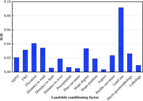
4.2. Importance of conditioning factors

Figure 6 plots the histogram of IGR values of the 15 factors. It has shown that the values of all factors are greater than zero, indicating that these factors have a certain contribution to the modelling of landslide susceptibility. Among these factors, land use is the most important factor, followed by the elevation and slope degree, suggesting these factors contributing greatly to the model. By contrast, the IGR values of the distance to fault, annual rainfall, plan curvature, and aspect are less than 0.01, which make little contribution to the model.

Figure 6. IGR of the landslide conditioning factors.

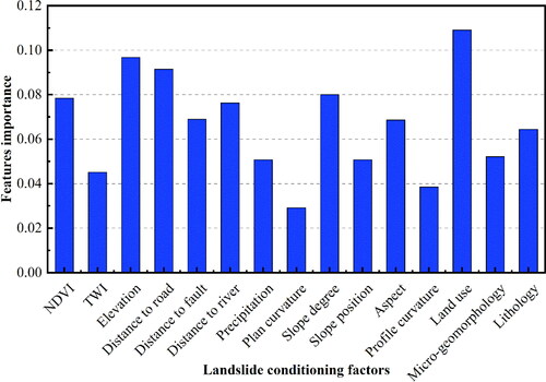
Due to the nature of the RF model, the importance of the fifteen factors is also obtained using the RF model based on the training data. The results are shown in Figure 7, which are basically consistent with those of IGR. Land use is still the most important factor, while only the order of some middle important factors has changed. Hence, in the following analyses, all landslide conditioning factors selected above are further used for landslide susceptibility modelling based on RF and LR. However, for AFM, the selected 14 factors which exclude the slope position are kept for the following analysis due to the sensitivity of the AFM model to the multicollinearity of the factors, as analyzed above.

Figure 7. Importance score of landslide conditioning factors for RF.

4.3. Landslide susceptibility maps

With the selected conditioning factors and recorded landslides data, the LSM models are first built by the proposed AFM and RF, and LR methods. Then, the landslide susceptibility maps are produced based on these susceptibility models by providing the landslide susceptibility indices (LSIs) for all pixels in the whole study area.

4.3.1. Landslide susceptibility map based on AFM

Since AFM is used to solve the classification task in this study, the logarithmic loss function is used as the loss function. The adaptive gradient algorithm is used as the optimizer to train the AFM model. Through parametric analyses on hyperparameters, it is found that the hyperparameter that has the greatest influence on AFM performance is ‘epochs’, which is the number of times to use all training sets. When the ‘epochs’ reaches about 100, the continuous increase of epochs will lead to over-fitting of the model and reduces the AUC value of the test set. Other hyperparameters, such as the attention size and dropout, do not show such strong correlations with the model performance indicator, AUC. Table 4 shows the hyperparameters finally adopted after the analyses.

Table 4. Hyperparameters in the AFM model.

Hyperparameters	Values
attention size	8
dropout	0
epochs	100
l2_reg_linear	1e-5
l2_reg_embedding	1e-5
l2_reg_att	1e-5

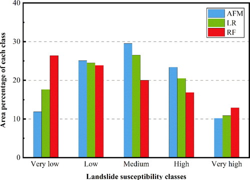
Landslide susceptibility map is an effective tool for land allocation decisions. After the training of the AFM model, the maps for the area are generated by calculating the LSIs through the model, as shown in Figure 8(a). The LSIs are classified using the Jenks natural break method into five categories: very low (0.00–0.316), low (0.316–0.406), medium (0.406–0.488), high (0.488–0.582), and very high (0.582–1). According to statistics of the LSIs shown in Figure 9, the medium class has the largest area (29.50%), followed by low (25.09%), high (23.38%), very low (11.84%), and very high (10.19%).

Figure 8. Landslide susceptibility maps: (a) AFM; (b) LR; (c) RF.

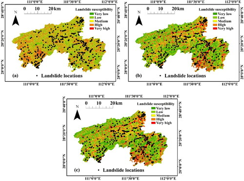
Figure 9. Area percentages of different landslide susceptibility classes for AFM, LR, and RF models.

4.3.2. Landslide susceptibility maps based on RF and LR

This part presents the landslide susceptibility maps produced by the LR and RF models. The LR model is implemented using the Python package scikit-learn 0.21. For a better model performance, it is necessary to determine appropriate hyperparameters, which are obtained through Bayesian optimization. The parameters are listed in Table 5. After the parameters are determined, the model is trained with the training dataset. Then, the LSIs in the whole study area are calculated by using the trained LR model to produce the landslide susceptibility map, as shown in Figure 8(b). In the map, the LSIs for all pixels are also classified into five classes: very low (0.000–0.089), low (0.089–0.245), medium (0.245–0.413), high (0.413–0.595), and very high (0.595–0.948) using the natural break method. The area percentage for each class is also shown in Figure 9. The figure shows that the medium class has the largest area proportion (26.53%), followed by the low (24.51%), high (20.50%), very low (17.60%), and very high (10.87%).

Table 5. Hyperparameters in LR and RF models.

Models	Hyperparameters	Values
LR	C	10
	solver	sag
	max-iter	10,000
RF	max-depth	15
	max-features	0.248
	min-samples-split	2
	n-estimators	400

For the RF model, a similar procedure for model training and prediction is implemented, and the corresponding hyperparameters are also summarized in Table 5. The predicted LSIs are also classified into five classes: very low (0.000–0.102), low (0.102–0.302), medium (0.302–0.517), high (0.517–0.733), and very high (0.733–0.999) using the natural break method. The area percentage of each class is shown in Figure 9. The very low class has the largest area (26.4%), followed by low (23.89%), medium (19.99%), high (16.84%), and very high (12.88%).

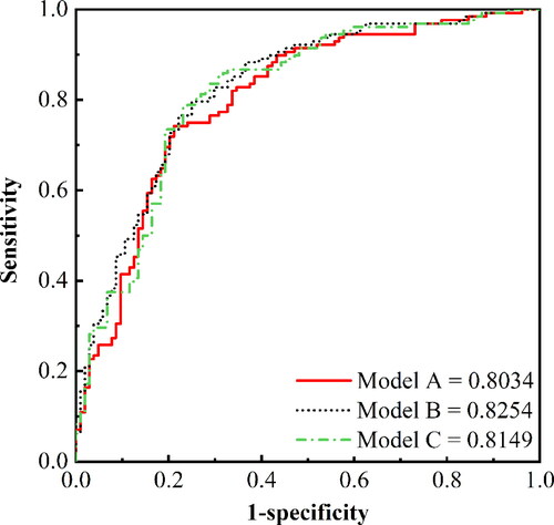
4.4. Model performance validation and comparison

As illustrated in the previous subsection, LR and RF models are applied to map the landslide susceptibility for a comparative purpose. Visually, the distribution patterns of landslides with high susceptibility levels generated from these three methods are different (Figure 8). According to the maps, it is seen that the very high susceptibility zones of LR and RF are mainly distributed in belts, which indicates that landslides are highly correlated with strip factors like distance to road. However, the high and very high zones of the AFM map are punctate and mainly concentrated in the southwest corner.

To further quantify and compare the predictive capability of the three maps, the prediction capabilities of the three constructed landslide models are evaluated using the validation data. The performance of the models is measured by the statistical indices and AUC values, which are shown in Table 6, while the ROC curves are plotted in Figure 10. The results show that the AFM model has the highest value (0.825) of AUC, which is slightly larger than that (0.819) of the RF model. LR has the worst performance, with an AUC value of 0.745. Besides, in terms of accuracy, RF and AFM have similar performance, i.e. 0.763 vs. 0.759, respectively, whereas LR performs the worst with an accuracy of 0.569. In terms of the Kappa index, RF is the highest, followed by AFM and LR. This observation indicates that when the classification threshold is 0.5, the performance of the AFM model will be worse than that of RF. Overall, it is acceptable for the three landslide models to implement LSM in the study area. However, the proposed AFM model performs the best in this study, which indicates that the map (Figure 8(a)) produced by AFM is more reliable.

Figure 10. ROC curves of the three models.

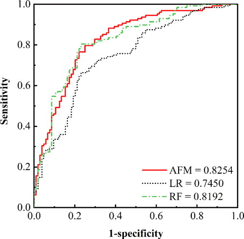
Table 6. Performance results of three models.

Model	AUC	TN	FP	FN	TP	Sensitivity	Specificity	Accuracy	Kappa
LR	0.745	73	31	35	93	0.727	0.702	0.716	0.668
RF	0.819	73	31	24	104	0.813	0.702	0.763	0.723
AFM	0.825	89	31	25	87	0.777	0.742	0.759	0.718

4.5. Statistical significance tests

To find out whether there are significant differences among the three models, the Friedman test has been performed on landslide susceptibility results (Dou et al. 2020a). Figure 11 uses three colours to represent the rank of different models and shows that significance is 0.00 (<0.05), which indicates that there are significant differences among the three models at a 5% significance level. However, it is worthwhile to point out that the Friedman test cannot identify which model is different from others. Hence, to gain more insights into the statistical differences between arbitrary pair of susceptibility models, the Wilcoxon signed-rank test is further conducted on the susceptibility results. The results are shown in Table 7. It is observed that any two pairs of the three models are statistically significantly different because at a 5% significant level the p value is less than 0.05 and the $z$ value exceeds the critical value of (–1.96 and +1.96).

Figure 11. Friedman analysis of variance by ranks.

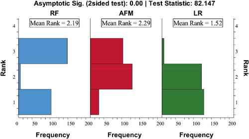
Table 7. Results of the Wilcoxon signed-rank test (two-tailed).

Pair-wise model	$\mathit{z}$ value	$\mathit{p}$ value	Significance
AFM vs. RF	–2.180	0.029	Yes
AFM vs. LR	–12.071	0.000	Yes
RF vs. LR	$+$3.197	0.001	Yes

5. Discussions

In multicollinearity analysis, VIF is often used in literature to evaluate multicollinearity, with a threshold of 10. Factors with VIF beyond the threshold are deleted from the original factors set (Chen and Chen 2021). Since the AFM model considers interactions of two factors, which may be more sensitive to multicollinearity, we implemented three comparative models to find out the VIF threshold for AFM. The results show that the threshold of AFM is about three, which finally removes the slope position from the original selected 15 landslide conditioning factors. Note that as more and more new models are applied to the LSA field, it is suggested that when researchers using a new model, they may need to try a new threshold for VIF. Since a new model may have different principles compared to those commonly used models, which may lead to different sensitivities to multicollinearity, continuing to use the available threshold of VIF without testing would affect the reliability of the results. In addition, it is found that land use is the most important factor in assessing landslide susceptibility based on IGR and RF in the current case study, which is consistent with Lu et al. (2015). Lu et al. (2015) believed that land use has an important influence on the triggering, stabilization, and activation of landslides. The potential reason may be that with the increase of human economic activities, land use and original soil properties change, leading to the occurrence of landslides. Avila et al. (2021) also explained through the mechanical model that the change of land use type and the reduction of vegetation would induce landslides. If multi-temporal data are available, it is possible to do a spatio-temporal analysis of landslides and land use types, so that the relationship between them could be more clear.

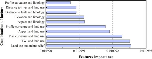
An important outcome of this study is that the proposed AFM provides the weights for different combinations of factors. Figure 12 plots the largest ten weights in descending order by histograms. It can be seen from the figure that the combination of land use and micro-geomorphology (i.e. micro-relief) contributes the most to the landslide susceptibility of the study area, followed by the (TWI, land use), (plan curvature, land use), (aspect, land use), (profile curvature, land use), (aspect, lithology), (elevation, lithology), (distance to fault, lithology), (distance to river, land use), and (profile curvature, lithology). This indicates that human engineering activities play an important role in inducing landslides in the area. Interestingly, plan curvature and profile curvature can affect the susceptibility results when they are interacted with land use, although they rank the lowest in the importance analysis of single factors by IGR and RF. This implies that AFM can explore the potential contributions of some factors and consider the influence of factors interaction on landslide occurrence, thereby yielding better landslide susceptibility results. Another important finding from the proposed method is that different weights of different combinations of interacted features only have minimum differences. The difference between AFM and the general linear model is that AFM considers the crossing features with specific weights given by the attention network. Because of the large number of crossing features, the slight difference between weights will accumulate and affect the results. It is the small difference between weights that makes the AFM perform better than the general linear model like LR.

Figure 12. Rank of the top 10 combinations of factors in attention score.

Based on different metrics of the landslide susceptibility model, the performance of LR is generally worse than RF and AFM, while the performance difference between AFM and RF depends on the evaluation index used. In the literature, AUC is the most used and accepted index (Dai and Xu 2013; Huang et al. 2020; Yi et al. 2020; Dou et al. 2020a). Overall, the AUC value of the AFM model is higher than those of the RF and LR models, suggesting that the AFM model is better than RF and LR models in the binary classification task. It should be noted that AFM can be used for sparse data, that is, training data is scarce and high dimensional (Xiao et al. 2017). By contrast, according to Breiman (2001), the performance of RF is not ideal in a data-sparse environment.

In the past few years, researchers have put a lot of effort into the selection of algorithms for LSM, but there still lacks a unified agreement on which method is the best (Wang et al. 2015; Chen et al. 2017; Dou et al. 2019). Recently, a few researchers have also tried to adopt novel deep learning (DL) models, such as convolutional neural networks (Sameen et al. 2020; Yi et al. 2020), to find new solutions. Dou et al. (2020b) found that unlike machine learning models, DL models are not affected by sampling strategies, demonstrating the advantages of DL. Future experiments can be done to see if the AFM model achieves this effect through the mechanism of attention in DL. In DL models, the relationship between each factor can only be expressed implicitly by multi-layer neurons, and cannot be shown as an AFM model, so the interpretability of the model is weak. Nevertheless, compared with DL models, there are also some limitations in AFM model. For example, owing to the final weighted accumulation, the quadratic terms in AFM do not carry out a deeper network to learn the nonlinear crossover features. Hence, AFM does not give full play to the advantages of DL. It is, however, expected that if AFM is combined with the advantage of DL in future work, better LSM results might be achieved.

6. Summary and conclusions

This paper has implemented an AFM model that can consider the interactions between factors to produce a more accurate susceptibility map for Anhua County, China, which makes it different from the available studies in the literature. The AFM enhances the traditional FM model by introducing an attention machine of DL, which improves not only the representation ability but also the interpretability of the FM model.

The performance of the proposed AFM method is systematically compared with two commonly used machine learning models of LR and RF by AUC values and statistical indices. Compared with the LR model and RF model, the AFM model has the highest predictive ability and can reflect the weight of the combination of factors, which can better explain the underlying causes of landslides in the area. The AFM model has an AUC value of 0.825, as shown in Fig. 10 and an accuracy rate of 0.759, which is a promising mapping technique for landslide susceptibility. These results may be helpful to decision-makers and land planning in landslide-prone areas like Anhua County.

Acknowledgement

The financial support is greatly acknowledged.

Disclosure statement

No potential conflict of interest was reported by the authors.

Additional information

Funding

The work described in this paper was funded by grants from the National Natural Science Foundation of China (Project No. 41902291), the Natural Science Foundation of Hunan Province, China (Project No. 2020JJ5704), the Hunan Provincial Innovation Foundation for Postgraduate (Project No. CX20200236), the Fundamental Research Funds for Central South University (Project No. 2020zzts651), the Open Research Fund Program of Key Laboratory of Metallogenic Prediction of Nonferrous Metals and Geological Environment Monitoring (Central South University), Ministry of Education (Project No. 2017YSJS11) and the Scientific Research Program of the Hunan Education Department (Project No. 19C1113).

References

- Aleotti P, Chowdhury R. 1999. Landslide hazard assessment: summary review and new perspectives. Bull Eng Geol Env. 58 (1):21–44.
- Avila FF, Alvala RC, Mendes RM, Amore DJ. 2021. The influence of land use/land cover variability and rainfall intensity in triggering landslides: a back-analysis study via physically based models. Nat Hazards. 105(1):1139–1161.
- Ayalew L, Yamagishi H. 2005. The application of GIS-based logistic regression for landslide susceptibility mapping in the Kakuda-Yahiko Mountains, Central Japan. Geomorphology. 65(1–2):15–31.
- Bai S, Wang J, Zhang Z, Cheng C. 2012. Combined landslide susceptibility mapping after Wenchuan earthquake at the Zhouqu segment in the Bailongjiang Basin, China. Catena. 99:18–25.
- Breiman L. 2001. Random forests. Mach Learn. 45(1):5–32.
- Chen W, Xie X, Wang J, Pradhan B, Hong H, Bui DT, Duan Z, Ma J. 2017. A comparative study of logistic model tree, random forest, and classification and regression tree models for spatial prediction of landslide susceptibility. Catena. 151:147–160.
- Chen X, Chen W. 2021. GIS-based landslide susceptibility assessment using optimized hybrid machine learning methods. Catena. 196:104833.
- Dai J, Xu Q. 2013. Attribute selection based on information gain ratio in fuzzy rough set theory with application to tumor classification. Appl Soft Comput. 13(1):211–221.
- Dehnavi A, Aghdam IN, Pradhan B, Morshed Varzandeh MH. 2015. A new hybrid model using step-wise weight assessment ratio analysis (SWARA) technique and adaptive neuro-fuzzy inference system (ANFIS) for regional landslide hazard assessment in Iran. Catena. 135:122–148.
- Dou J, Yunus AP, Bui DT, Merghadi A, Sahana M, Zhu Z, Chen C-W, Han Z, Pham BT. 2020a. Improved landslide assessment using support vector machine with bagging, boosting, and stacking ensemble machine learning framework in a mountainous watershed, Japan. Landslides. 17(3):641–658.
- Dou J, Yunus AP, Merghadi A, Shirzadi A, Nguyen H, Hussain Y, Avtar R, Chen Y, Pham BT, Yamagishi H. 2020b. Different sampling strategies for predicting landslide susceptibilities are deemed less consequential with deep learning. Sci Total Environ. 720:137320.
- Dou J, Yunus AP, Tien Bui D, Merghadi A, Sahana M, Zhu Z, Chen C-W, Khosravi K, Yang Y, Pham BT. 2019. Assessment of advanced random forest and decision tree algorithms for modeling rainfall-induced landslide susceptibility in the Izu-Oshima Volcanic Island, Japan. Sci Total Environ. 662:332–346.
- Guzzetti F, Carrara A, Cardinali M, Reichenbach P. 1999. Landslide hazard evaluation: a review of current techniques and their application in a multi-scale study, Central Italy. Geomorphology. 31(1–4):181–216.
- Hu Q, Zhou Y, Wang S, Wang F. 2020. Machine learning and fractal theory models for landslide susceptibility mapping: case study from the Jinsha River Basin. Geomorphology. 351:106975.
- Huang F, Cao Z, Guo J, Jiang S-H, Li S, Guo Z. 2020. Comparisons of heuristic, general statistical and machine learning models for landslide susceptibility prediction and mapping. Catena. 191:104580.
- Hung LQ, Van NTH, Duc DM, Ha LTC, Van Son P, Khanh NH, Binh LT. 2016. Landslide susceptibility mapping by combining the analytical hierarchy process and weighted linear combination methods: a case study in the upper Lo River catchment (Vietnam). Landslides. 13(5):1285–1301.
- Juliev M, Mergili M, Mondal I, Nurtaev B, Pulatov A, Hubl J. 2019. Comparative analysis of statistical methods for landslide susceptibility mapping in the Bostanlik District, Uzbekistan. Sci Total Environ. 653:801–814.
- Lee M-J, Park I, Lee S. 2015. Forecasting and validation of landslide susceptibility using an integration of frequency ratio and neuro-fuzzy models: a case study of Seorak mountain area in Korea. Environ Earth Sci. 74(1):413–429.
- Lin G-F, Chang M-J, Huang Y-C, Ho J-Y. 2017. Assessment of susceptibility to rainfall-induced landslides using improved self-organizing linear output map, support vector machine, and logistic regression. Eng Geol. 224:62–74.
- Lu P, Bai S, Casagli N. 2015. Spatial relationships between landslide occurrences and land cover across the Arno River Basin (Italy). Environ Earth Sci. 74(7):5541–5555.
- Merghadi A, Yunus AP, Dou J, Whiteley J, ThaiPham B, Bui DT, Avtar R, Abderrahmane B. 2020. Machine learning methods for landslide susceptibility studies: a comparative overview of algorithm performance. Earth Sci Rev. 207:103225.
- Pereira S, Santos PP, Zêzere JL, Tavares AO, Garcia RAC, Oliveira SC. 2020. A landslide risk index for municipal land use planning in Portugal. Sci Total Environ. 735:139463.
- Pham BT, Nguyen-Thoi T, Qi C, Phong TV, Dou J, Ho LS, Le HV, Prakash I. 2020. Coupling RBF neural network with ensemble learning techniques for landslide susceptibility mapping. Catena. 195:104805.
- Pham BT, Prakash I, Chen W, Ly H-B, Ho LS, Omidvar E, Tran VP, Tien Bui D. 2019. A novel intelligence approach of a sequential minimal optimization-based support vector machine for landslide susceptibility mapping. Sustainability. 11(22):6323.
- Reichenbach P, Rossi M, Malamud BD, Mihir M, Guzzetti F. 2018. A review of statistically-based landslide susceptibility models. Earth Sci Rev. 180:60–91.
- Rendle S. 2011. Factorization machines. IEEE International Conference on Data Mining; Sydney, Australia.
- Sameen MI, Pradhan B, Lee S. 2020. Application of convolutional neural networks featuring Bayesian optimization for landslide susceptibility assessment. Catena. 186:104249.
- Sara F, Silvia B, Sandro M. 2015. Landslide inventory updating by means of Persistent Scatterer Interferometry (PSI): the Setta basin (Italy) case study. Geomatics Nat Hazards Risk. 6(5–7):419–438.
- Tang W, Lu T, Li D, Gu H, Gu N. 2020. Hierarchical attentional factorization machines for expert recommendation in community question answering. IEEE Access. 8:35331–35343.
- Wang HJ, Xiao T, Li XY, Zhang LL, Zhang LM. 2019. A novel physically-based model for updating landslide susceptibility. Eng Geol. 251:71–80.
- Wang L-J, Guo M, Sawada K, Lin J, Zhang J. 2015. Landslide susceptibility mapping in Mizunami City, Japan: a comparison between logistic regression, bivariate statistical analysis and multivariate adaptive regression spline models. Catena. 135:271–282.
- Wang Y, Feng L, Li S, Ren F, Du Q. 2020. A hybrid model considering spatial heterogeneity for landslide susceptibility mapping in Zhejiang Province, China. Catena. 188:104425.
- Weiss A. 2001. Topographic position and landforms analysis. ESRI User Conference; San Diego, CA.
- Xiao J, Ye H, He X, Zhang H, Wu F, Chua TS. 2017. Attentional factorization machines: learning the weight of feature interactions via attention networks. In 26th International joint conference on artificial intelligence (IJCAI), pp. 3119–3125.
- Xie Z, Chen G, Meng X, Zhang Y, Qiao L, Tan L. 2017. A comparative study of landslide susceptibility mapping using weight of evidence, logistic regression and support vector machine and evaluated by SBAS-InSAR monitoring: Zhouqu to Wudu segment in Bailong River Basin, China. Environ Earth Sci. 76(8):313.
- Yi Y, Zhang Z, Zhang W, Jia H, Zhang J. 2020. Landslide susceptibility mapping using multiscale sampling strategy and convolutional neural network: a case study in Jiuzhaigou region. Catena. 195:104851.
- Youssef AM, Al-Kathery M, Pradhan B. 2015. Landslide susceptibility mapping at Al-Hasher area, Jizan (Saudi Arabia) using GIS-based frequency ratio and index of entropy models. Geosci J. 19(1):113–134.
- Zhang S, Li C, Peng J, Peng D, Xu Q, Zhang Q, Bate B. 2021. GIS-based soil planar slide susceptibility mapping using logistic regression and neural networks: a typical red mudstone area in southwest China. Geomat Nat Hazards Risk. 12(1):852–879.
- Zhao X, Chen W. 2020. Optimization of computational intelligence models for landslide susceptibility evaluation. Remote Sens. 12(14):2180.