A comparative evaluation of machine learning algorithms and an improved optimal model for landslide susceptibility: a case study

Abstract

In this study, four representative machine learning methods (support vector machine (SVM), maximum entropy (MaxEnt), random forest (RF), and artificial neural network (ANN)) were employed to construct a landslide susceptibility map (LSM) in Xulong Gully (XLG), southwest China. The models were subsequently compared in order to select the best-performing model. This model was further improved to optimize the machine learning method. A total of 16 layers were extracted from the collected data and employed as conditional factors for the correlation analysis and subsequent modelling. The LSMs were then divided into four levels (very high susceptibility (VH), high susceptibility (H), moderate susceptibility (M) and low susceptibility (L)). The results were verified by receiver operating characteristic (ROC) curves, Root Mean Squared Error (RMSE) and Frequency Ratio (FR). The higher of the area under ROC curve (AUC) and the lower the RMSE, the more accurate and stable the performance. Following the factor performance analysis, the optimal SVM model was linearity improved to the Trace Ratio Criterion (TRC)-SVM, with a better performance and the ability to overcome the factor defect. The comprehensive comparisons and proposed LSM can support future research, as well as local authorities in the development of landslide remission strategies.

Keywords:

• Landslide susceptibility
• support vector machine
• maximum entropy
• random forest
• artificial neural network
• Xulong gully

1. Introduction

Geological hazards, a common occurrence in Southwest China, can have a devastating impact on environmental systems and sustainable development (Bai et al. 2012). Approximately 1046 geological hazards occurred in 2019 in Southwest China, reaching 16.90% of the nationwide total. A total of 68.27% of these were landslides, causing 89 deaths, 9 missing persons, and CNY 1.7 billion (equal to USD～0.24 billion by April 2020 conversion) in financial damage. Unfortunately, landslides are natural disasters that cannot be avoided and are triggered by numerous factors (e.g., abundant rainfall, complex geo-environmental settings, high-frequency earthquakes, etc.) in mountainous communities (Parker et al. 2011; Gorum et al. 2013; Nsengiyumva and Valentino 2020).

Extensive research has been performed on the problems caused by landslides, both directly or indirectly. Direct problems are usually investigated via point-to-point monitoring, while indirect methods focus on natural factors to analyze the landslide formation mechanism (Xu et al. 2014; Fang et al. 2020; Yuan et al. 2021). For example, streams play an important role in the formation of unstable slopes in mountainous areas (Vojteková and Vojtek 2020). Physical models are commonly employed in landslide analysis to account for streams (e.g., examining the role of vegetation via slope stability models or man-made factors) (Pham et al. 2016; Wiesmair et al. 2017). Landslides occur at a high frequency along transportation lines, causing damage to communities, property, and resulting in the loss of life (Hong et al. 2018; Jones et al. 2020). Therefore, effective guidelines for landslides risk assessments and risk zoning are necessary (Maloney et al. 2020). Geological hazard model outputs should be presented with a complete hazard evaluation, including the location and scale of the geological hazard (Saha et al. 2005). A susceptibility study of geological hazards can provide information about the stability of areas and the probability of predictions in order to plan for disaster governance and further engineering activities (Khamkar and Mhaske 2019).

Much effort was made to produce landslide susceptibility maps in the early 1970s based on qualitative research (Babb and Bliss 1974). In particular quantitative assessments of landslide susceptibility expanded following the development of Autosnap and the advancement of data acquisition and analytical approaches (Roth 1983). Booth conducted a regional landslide susceptibility evaluation based on the aspect, slope gradient, and bedrock elements contributing to land management (Booth et al. 1984). In 1989, Jibson and Keefer created a geological hazard susceptibility map using over 200 large geological hazards at the edge of the Mississippi Plain via discriminant and multiple linear regression analyses (Jibson and Keefer 1989). Previous work has proposed adopting a discrete combination of geological and geomorphic parameters to calculate landslide susceptibility. In addition, the matrix evaluation method has been introduced to evaluate slope stability in large scale mountainous areas. More recently, GIS techniques have become a common feature in landslide susceptibility mapping (De Ploey et al. 1995; Pannatier et al. 2009), which can be grouped into two components: linear regression analysis and nonlinear regression analysis. Logistic regression models (Bui et al. 2016) are the most widely used of linear regression analysis. Neural networks (Cao et al. 2019) is a kind of nonlinear regression approaches and artificial neural network (ANN) (Tian et al. 2019) as one of the major neural network algorithms is developed on the basis of neural network. Model algorithm accuracy and diversification have improved geological hazard susceptibility mapping, particularly with the rapid growth of computer technology and the popularization of GIS techniques (Tehrani et al. 2021).

Geological hazard susceptibility mapping typically includes physical modelling, statistical analysis, and software calculations (Pourghasemi and Rahmati 2018). The physical models require a large number of simulation experiments, as well as analyzing the engineering geological conditions and slope of the field, which can prove to be difficult for large scale areas (Prasad et al. 2016). Statistical analysis generally calls for the parameterization of the structure model and the integration with machine learning techniques to determine the relationship between factors (Vasu and Lee 2016). Machine learning methods are efficient and can help to predict disaster risk and decrease disaster costs. Thus regions vulnerable to natural hazards should adopt detailed assessments that are implemented accordingly (Goetz et al. 2015; Nhu et al. 2020; Jiang et al. 2021). In this regard, susceptibility is often used in natural hazards to analyze and predict the relevant human activities, environment, and geology on a such scale as it not only considers the multivariate limitation but also the nonlinearity (Tonini et al. 2020). Despite its importance in landslide susceptibility mapping there are currently no concerted standards for the selection of machine learning methods in geological hazard susceptibility mapping (Pourghasemi and Rahmati 2018; Li et al. 2020). Numerous machine learning models have been applied for geological hazard susceptibility mapping in recent years, making valuable progress. For example, random forest (RF) can outperform general statistical and heuristic analysis models (Huang et al. 2020), and also improves on the classification results of decision trees (Zhang et al. 2017). Thus, we employ RF in this paper. Moreover, ANNs and support vector machine (SVMs) are typically adopted in research on susceptibility mapping and we also compare them here (Chen et al. 2020; Peethambaran et al. 2020). Maximum entropy (MaxEnt) is a widely used statistical-probabilistic machine learning algorithm that contains more universal generality (Kariminejad et al. 2019; Pandey et al. 2020) than other machine learning algorithms such as multiple adaptive regression splines (MARS) (Arabameri et al. 2019) and the adaptive neuro-fuzzy inference system (ANFIS) (Polykretis et al. 2019). RF, ANN and SVM also exhibit similar performances (Chen et al. 2017; Arabameri et al. 2020). However, the resulting accuracy is strongly influenced by the extent and training procedure. Further, research is required to determine which model is more suitable for mountainous geological hazard susceptibility assessments.

Despite their important research significance, landslides are often overlooked. In the present study, four linear and nonlinear machine learning algorithms were selected to develop landslide susceptibility maps: MaxEnt, SVM, ANN and RF. These high-accuracy and reliable algorithms have recently been utilized in landslide susceptibility studies across the Xulong gully (XLG) of Southwest China as well as other areas. We present a detailed classification of the impact factors of each algorithm to compare. Next introduced the trace ratio criterion (TRC) algorithm into the optimal algorithm to make a majorization. We denote the proposed algorithm TRC-SVM following the improved SVM algorithm and evaluate its performance using the receiver operating characteristic (ROC) curves, Root Mean Squared Error (RMSE) and Frequency Ratio (FR) as previous. This work combines remote sensing datasets and extensive field surveys of landslides and collapses, providing material for mudslides and amplifying its size. Our results determine the possible damming induced by a hydroelectric station close to XLG following the occurrence of a mudslide during the research period. The comparison of the four machine learning algorithms for landslide susceptibility provides a considerable contribution to the five villages in XLG. Furthermore, the optimal algorithm for landslide susceptibility mapping can identify and delineate landslide prone zones, which is beneficial to government decision-making and disaster avoidance.

2. Study area and data collection

2.1. Study area

Xulong gully (XLG) lies in the Jinshajiang Basin with a size of 55.6 km² and surrounded by five villages between the Qinghai-Tibet Plateau and Sichuan-Yunnan Plateau, southwest China (N 28°43′57″, W 99°7′56″to N 26°49′22″, W 99°13′29″) (Figure 1). The area contains one main gully and 13 branch gullies with hundreds of rockfalls and landslides. The elevation ranges between 2100 and 4800 m, with the highest elevation located in the northwest region. Mountains at higher and lower elevations have steep ridges and sheer inclines with horns forming V-type river valleys. The area generally exhibits a subtropical arid valley climate that varies greatly in time and space, with an average annual precipitation of approximately 363.3 mm, wet and rainy weather in winter and sunshine and wind in the summer. In addition, the high mountain canyon topography, heterogenous geo-environment and a variable climate result in the frequent occurrence of geological disasters.

Figure 1. Location of the study area in China (left: Google Maps), the Xulong gully (right).

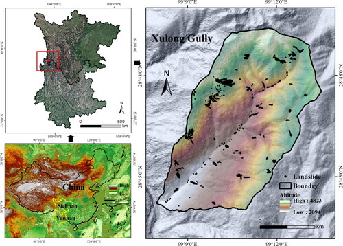
XLG is located in the northern Hengduan Mountains, a part of the SE Qinghai-Tibet Plateau of China, with a SW trend. The study area is crossed by crumbled rocks and legions of faults, including the riff-Riyu, Xumai-Niwu, and Zeng-Datong faults, etc. These three faults are the key contributors to the intermediate part of the Jinsha River faulting junction zone, which stretches from the north to south, with the riff-Riyu fault being the most fragmented, distorted, and deepest of the three. This fault is geologically located in a different geologic unit, whereby gneiss and greenschist of the Jinsha River Ophiolite suite (DTJ) from the broadest spectrum, followed by dolomite of the Silurian-Yongren Group (S₂γ), garnet-mica schist and marble of the third Xiongsong Group (P_t2X³), conglomerate and sandstone of the Triassic (T₃j), and lastly terraced fields and alluvial fans distributed in the Quaternary. This forms a complicated system of geological faults with a diversity of delicate rock textures under the influence of variable temperatures and active crustal movement, including landslides and rockfalls.

2.2. Data collection

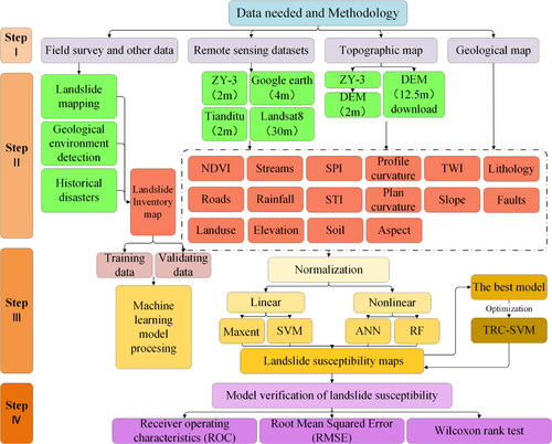
The current study presents the application of different data sources used in landslide susceptibility mapping. Datasets were obtained from the interpretation of remote sensing images downloaded from Google Earth, with a 4 m resolution and referenced using a Tianditu on-line map and a Ziyuan-3 (ZY-3) satellite image with a higher resolution of 2 m. Field survey validations were then performed during the study, including the collection of reliable landslide positions, and road, water, and land-use data. Furthermore, information on historical landslides was collected via interviews with the regional annuals, and the local government. Precipitation data was provided by the China Meteorological Administration, a digital elevation model (DEM) of 2 m resolution was obtained from a ZY-3 satellite image, and a 12.5 m resolution image was taken from Earthdata, a website sharing information service by NASA’s EOSDIS (Earth Observing System Data and Information System). We then digitized the lithology and structure from traditional maps with a scale of 1:50000. All datasets were stored in the same digital shape with a UTM-Zone 47 projection and WGS-84 datum. Figure 2 presents the methodological approach.

Figure 2. Architecture of the datasets, their derived products, and their usage.

2.3. Inventory map and extracted factors

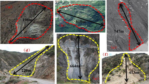
A landslide inventory map is one of the most important elements of a landslide susceptibility assessment (Salles and Duclaux 2015; Sun et al. 2020). Landslides typically occur in areas where they have already taken place, with a similar slope, lithology, elevation, fault environment, and so on (Cama et al. 2020). We created a landslide inventory map to demonstrate such relationships based on previous work. The on-line map and ZY-3 imagery were employed to identify landslide features (e.g., round-armchair shapes, long strips, scarps, divergent texture, etc.; Figure 3 (a-c)) (Chang et al. 2020; Godone et al. 2020) and the field investigation was performed to ensure reliability (Figure 3 (d-f)). Historical hazards from the Bureau of Natural Resources were combined with the multidimensional hazards to create a landslide inventory map with the 286 disasters shown in Figure 1. We then converted the 286 landslide polygons into points to ensure that each point is in a grid and each grid contains at least a single feature cell. A total of 7,938 points remained after the removal of invalid points and was denoted as the landslide sample. Such a selection not only makes these points replace the complete landslide information, but also improves the stability of the model by increasing the number of training samples. We employ 70% of the sample to train the model and 30% for the validation. The same amount of pseudo absence data was created by randomly dividing the points into 70% and 30% groups as the training data and validation data, respectively when required. The study area was made up of 583,615 pixels, 5,246 determined as landslide pixels and 5,246 selected as non-landslide pixels.

Figure 3. Examples of collapses and landslides: (a)-(c) landslide from an optical image (d) - (f) are landslides from field investigation.

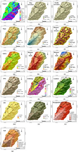
In order to evaluate the factors affecting landslides, we selected four groups of topographical, geological, hydrological, and landuse variables according to the empirical consensus on the interaction between landslide locations. The variables include elevation, slope aspect, slope angle, plan curvature, profile curvature, lithology, distance from faults, distance from streams, distance from roads, landuse, normalized difference vegetation index (NDVI), topographic wetness index (TWI), stream power index (SPI), sediment transport index (STI), soil and precipitation (Figure 4). The seven geological layers (slope aspect, plan curvature, profile curvature, slope angle, elevation, SPI, and STI) were obtained from the DEM using ArcGIS 10.2 (ESRI) (Figure 4(a-e), (m-n)). Similarly, ArcGIS was employed to extract distance maps from the remote sensing interpretation results, the Tianditu online map, and the DEM (Figure 4(f) (h) (i)). NDVI (Figure 4(g)) was determined from band calculations of Landsat 8 imagery in ENVI 5.3 (Exelis Visual Information Solutions) as follows: $$\mathrm{NDVI}=\left(B5-B4\right)/\left(B5+B4\right),$$ where B4 and B5 are the red and near-infrared bands. We also calculated TWI (Figure 4(j)) via ArcGIS, which combines precipitation data (Figure 4(o)) from the China Meteorological Administration to precisely determine the impact of rainfall. Soil dataset (Figure 4(p)) was obtained from the National Earth System Science Data Center. Lastly, a seven-category landuse map was extracted by remote sensing image interpretation, containing residential, water, farmland, barren land, forest, grass, and snow-capped mountains (Figure 4(l)). All of these conditional factors were built in a 12.5 m grid.

Figure 4. Landslide casual factors: (a) Aspect; (b) Plan curvature; (c) Profile curvature; (d) Slope; (e) Elevation; (f) Distence to streams; (g) NDVI; (h) Distance to faults; (i) Distance to roads; (j) TWI; (k) Lithology; (l) Landuse; (m) SPI; (n) STI; (o) Precipitation; (p) Soil.

3. Methodology

The machine learning (ML) method is commonly applied for landslide susceptibility analysis thanks to its learning advantage over other data classification algorithms. It simulates the human mind to decide data affiliations based on the known data to modulates the relationships of data elements to inhibit and activate other data. Here, we select four linear (MaxEnt and SVM) and nonlinear (RF and ANN) methods. The decision boundary for the classification of linear methods must be a straight line, although they can also use the curve fitting sample. We compared and selected the most suitable algorithm of the study area for further improvements, thus establishing an ML-integrated feature extraction method to realize landslide susceptibility mapping. In this section, we introduce the application of the Pearson correlation coefficient to make a preliminary assessment among factors. The principles of the four machine learning methods are then introduced, followed by a description of the improved optimal. Finally, model validation is introduced.

3.1. Preliminary assessment of factors

The Pearson correlation coefficient was employed to compare the factors by measuring the linear relationship and distance variables between two factors: (1) $$r=\frac{N\sum x_i{y}_i-\sum x_i\sum y_i}{\sqrt{N\sum x_i^2-{\left(\sum x_i\right)}^2}\sqrt{N\sum y_i^2-{\left(\sum y_i\right)}^2}},$$(1) where N is the number of variable values. If r = 0, there is no linear correlation between x and y. The larger the absolute value of the correlation coefficient, the stronger the correlation; the closer the correlation coefficient is to 1 or −1, the stronger the correlation; and the closer the correlation coefficient is to 0, the weaker the correlation. The Pearson correlation coefficient compares different classes of factors that cannot be compared directly. The lower the correlation between factors, the higher the model reliability.

3.2. Model descriptions

3.2.1. Maximum entropy

Entropy is a measurement of information. Maximum entropy (MaxEnt) is based on the fundamental principle of preferring the known information to subjective data when we extrapolate the unknown. However, more information will decrease the information entropy. Therefore, the MaxEnt tenet is the most objective model with the highest information entropy based on the known data. This model can forge links between various impacts and the interplay of these impacts and landslides. MaxEnt provides a description of the emphasis of each factor and the corresponding contribution rates. Due to its automatic selection of parameters and operation with accutate forecasting, MaxEnt is now common in landslide predictions (Kornejady et al. 2017; Azareh et al. 2019).

Essentially, MaxEnt provides an estimate of probability. Information entropy in one system denotes a product of each possibility’s values and “log(possibility)”, then take its negative value such as Eq. (2)(2) $$H\left(P\right)=-\sum _{x}P\left(X\right)\hspace{0.17em}\text{log}\hspace{0.17em}P\left(X\right),$$(2) : (2) $$H\left(P\right)=-\sum _{x}P\left(X\right)\hspace{0.17em}\text{log}\hspace{0.17em}P\left(X\right),$$(2) where H(P) is the probability and P(X) is the information entropy.

The probability ranges between 0 and 1 and the log is lower than 0, thus when the negative is taken the entropy will be positive. We aim to determine P with the highest H (i.e., the highest entropy) and subsequently calculate the derivative of H(P) to obtain the extremum. For example, consider a system with n events and the probability of each event equal to p_i and the sum of events must be equal to 1: (3) $$H\left(P\right)=-\sum _{i=1}^n{p}_i\hspace{0.17em}\text{log}\hspace{0.17em}{p}_i,$$(3) with the constraint described as: (4) $${\sum }_{i=1}^n{p}_i=1.$$(4)

In order to satisfy Eqs. (3)(3) $$H\left(P\right)=-\sum _{i=1}^n{p}_i\hspace{0.17em}\text{log}\hspace{0.17em}{p}_i,$$(3) and (4)(4) $${\sum }_{i=1}^n{p}_i=1.$$(4) , we construct a Lagrange function: (5) $$L\left(p,\lambda \right)=-\sum _{i=1}^n{p}_i\hspace{0.17em}\text{log}\hspace{0.17em}{p}_i+\lambda \left(\sum _{i=1}^n{p}_i-1\right)$$(5)

Calculate its derivatives under the constraint to obtain final odds.

3.2.2. Support vector machine

A support vector machine (SVM) is employed for sorting possesses with high efficiency, identifying a hyperplane (Eq. (6)(6) $$f\left(x\right)=w^{T}x+b=0,$$(6) ) when working within a high-dimensional data space to perform classification tasks (Figure 5(a)). (6) $$f\left(x\right)=w^{T}x+b=0,$$(6) where w and b are straitjacket factors.

Figure 5. The diagram of SVM classification principle: (a) Map of linear classification; (b) Sketch map about linear classification of SVM.

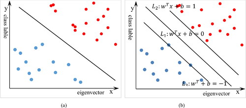
We define hyperplane L1, with two side planes L2 and L3. We call it the margin of the distance between L2 and L3 (Figure. 5(b)). There exists one best plane only, although there are many planes among L2 and L3 that for margin maximization denoted as the optimal face split. L1 is the optimal face split. We take several points at the nearest distance from L1 on L2 and L3 are samples. They help us classify so we call them support vectors (Pandey et al. 2020). The distance between the support vector and L1 is calculated as follows: (7) $$d=\frac{\left|w^{T}x+b\right|}{\Vert w\Vert },$$(7) thus, to calculate d, we must determine straitjacket factors w and b. In order to do this, we introduce a Lagrange multiplier αi ≥ 0 to get Eq. (8)(8) $$L\left(w,b,\alpha \right)=\frac{1}{2}{\Vert w\Vert }^2-\sum _{i=1}^n{\alpha }_i\left(1-y_i\left(w^T{x}_i+b\right)\right).$$(8) : (8) $$L\left(w,b,\alpha \right)=\frac{1}{2}{\Vert w\Vert }^2-\sum _{i=1}^n{\alpha }_i\left(1-y_i\left(w^T{x}_i+b\right)\right).$$(8)

Following the calculations, the equation consists of partial derivatives of w and b. For L, we obtain the values of w and b, and the resultant classification model can be described as: (9) $$f\left(x\right)=\mathit{sign}\left(w^{T}x+b\right)=\mathit{sign}\left(\sum _{i=1}^n{\alpha }_i{y}_i{x}_i^{T}x+b\right).$$(9)

SVM can be linear or nonlinear, depending on the presence of a kernel function. We chose a kernel function to maximize the accuracy and resolve nonlinear problems such as polymerization, radial basis function (RBF), and sigmoid. The training data could not be immediately sorted as it was linear in the actual assignment, thus the kernel function played an important role (Zhu and Blumberg 2002). The data was separated by multiple segmentation, where by the largest possible nearest distance from samples was used to segment a surface. The selection of a final hyperplane was then based on a linear algorithm.

3.2.3. Artificial neural networks

An artificial neural network (ANN) is a computer system that imitates the processes of the brain’s neurons. The ANN is considered as a biological neuron by analogy and includes the cell body, dendrite, axon, and synapse. Dendrite cells are inputs that receive signals from other cells, axons are outputs that send signals to other cells, and synapses are the interface of the inputs and outputs through which a signal passes from one nerve cell to another. The information from the inputs alters the neuron potential and accumulates continuously. The neuron is activated and a pulse is generated and transmitted to the next neuron when greater than a threshold (Wang et al. 2019). Figure 6 presents an example of ANN neuron.

Figure 6. The architecture of ANN.

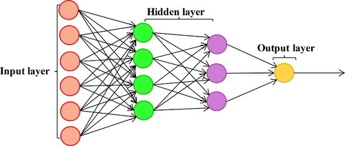
Neural network leaning is known as training, allowing the neural network to respond to the external environment in a new pathway. Each neural network has an activation function y = f(x), which is fit through a given x and y. ANNs are robust in training data, although training samples may contain errors that don’t have an effect on output. And ANNs can withstand a long training time, which depends on the number of weights, training samples, and the parameter settings (Dou et al. 2015); and the ANNs that used for output with objective function can be a discrete value, real value, or a vector of attributes for several real or discrete values. These advantages result in the strong applicability of ANNs in landslide susceptibility analysis.

3.2.4. Random forest

Random forest (RF) is the ensemble of numerous decision trees. Ensembles include boosting and bagging, and RF is an improvement of bagging. During the bagging process, the training data is divided into n new training data and an independent model is constructed on each data point of the new data. Finally, we integrate the results of these models with the number of n (Figure 7).

Figure 7. The principle chart of RF.

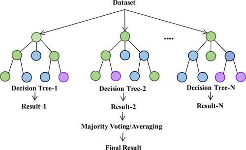
We select N and M to represent the number of training cases and features, respectively. The number of input features m denotes the decision result of a node in the decision tree. For each node, m features are randomly selected, and the decision of each node in the decision tree is determined based on these features. The optimal splitting mode is calculated based on the characteristics of m. Each tree is constantly pruned to complete the classification.

3.3. Improved optimal algorithm: TRC-SVM

The optimized SVM algorithm is denoted as the trace ratio criterion-support vector machine (TRC-SVM). The TRC-SVM is applied in feature extraction to reduce the data dimensionality via the trace ratio following the application of pretreatment factors through the branch bound method. The trace ratio algorithm is a typical feature selection algorithm of the filter model that widely employed in the feature selection of machine learning frameworks (Li et al. 2017). The traditional feature selection method calculates the score of a single feature to evaluate the advantages and disadvantages of all the features. The features with the highest score are selected to form feature subsets. However, the feature subsets obtained via this method are not optimal due to the presence of multiple features. TRC calculates the ratio of traces on two layers pair by pair, and the optimal feature subset is extended to several new layers. The new and original layer are then input into the SVM model following the determination of the optimal feature subset. Therefore, the features would give better performance to the energy of features by combining together (Wang et al. 2017). The TRC implements a new iterative method to directly calculate the score of the subset level in order to improve the optimization factor for SVM modelling.

Consider an original high-dimensional dataset x, x∈R^D, where D is the number of features per sample. Eq. (10)(10) $$\mathrm{y}=W^{T}x.$$(10) is employed to reduce the dimensions of original data set x to get new data set y. (10) $$\mathrm{y}=W^{T}x.$$(10)

The evaluation criteria of the feature subset is shown in Eq. (11)(11) $$\mathrm{J}\left(W_I\right)=\frac{{\sum }_{ij}{\Vert y_i-y_j\Vert }^2{\left(A_b\right)}_{ij}}{\sum _{ij}{\Vert y_i-y_j\Vert }^2{\left(A_w\right)}_{ij}},$$(11) : (11) $$\mathrm{J}\left(W_I\right)=\frac{{\sum }_{ij}{\Vert y_i-y_j\Vert }^2{\left(A_b\right)}_{ij}}{\sum _{ij}{\Vert y_i-y_j\Vert }^2{\left(A_w\right)}_{ij}},$$(11) where matrices A_w and A_b describe the within and between class relationships of the data, respectively. If x_i and x_j belong to the same class or are closely related to each other, the value of (A_w)_ij will be relatively large; if not, (A_w)ij will be relatively small. Thus we aim to minimize ${\sum }_{ij}{\Vert y_i-y_j\Vert }^2{\left(A_w\right)}_{ij}.$ Moreover, A_b describes the between class relationship of the data, and thus when selecting feature subsets, ${\sum }_{ij}{\Vert y_i-y_j\Vert }^2{\left(A_b\right)}_{ij}$ should be maximized. Eq. (12)(12) $$\mathrm{\varnothing }\left(I\right)=\arg {\mathit{max}}_{\mathrm{\varnothing }\left(I\right)}\frac{tr\left(W_I^{T}X{L}_b{X}_T{W}_I\right)}{tr\left(W_I^{T}X{L}_w{X}_T{W}_I\right)},$$(12) describes the feature subset with the highest score: (12) $$\mathrm{\varnothing }\left(I\right)=\arg {\mathit{max}}_{\mathrm{\varnothing }\left(I\right)}\frac{tr\left(W_I^{T}X{L}_b{X}_T{W}_I\right)}{tr\left(W_I^{T}X{L}_w{X}_T{W}_I\right)},$$(12) where L_w and L_b are Laplacian coefficients, L_w = D_w - A_w, ${\left(D_w\right)}_{ij}=\sum _j{\left(A_w\right)}_{ij}$ and L_b = D_b-A_b, ${\left(D_b\right)}_{ij}=\sum _j{\left(A_b\right)}_{ij}.$ The feature subset is obtained following a series of operations in order to overcome the factor defects. The feature subset is used in the machine learning algorithm as a conditional factor.

3.4. Assessing model performances

It is an essential process to measure the performance of model. Here, we employed the following factors for performance: the receiver operating characteristic (ROC) curve, the area under ROC curve (AUC), the root mean squared error (RMSE), and the frequency ratio (FR).

The ROC curve can effectively describe the classification performance of a classifier for samples with an uneven distribution (Vakhshoori and Zare 2018). The ROC space defines the false positive rate (or sensitivity) as the X-axis and the true positive rate (or specificity) as the Y-axis. We can get different data pairs by adjusting the classification threshold of the classifier. These data pairs are the ROC data points. The area below the ROC curve is denoted as the AUC, which is also commonly used to evaluate the classification accuracy of the model. The closer the AUC is to 1, the better the performance (Marjanović 2013).

The RMSE denotes the square root of the ratio of the deviation between the predicted and true values and the number of observations (Moayedi et al. 2019). It is used to measure the deviation between the observed and true values, thus the larger the value, the more instable the performance.

The FR is a map validation technique, calculated using the ratio of the area (%) of landslide pixels per class to the total area (%) of pixels per class. A significant increase in the ratio from low to high susceptibility, denotes a strong classification performance.

4. Results

4.1. Factor assessments

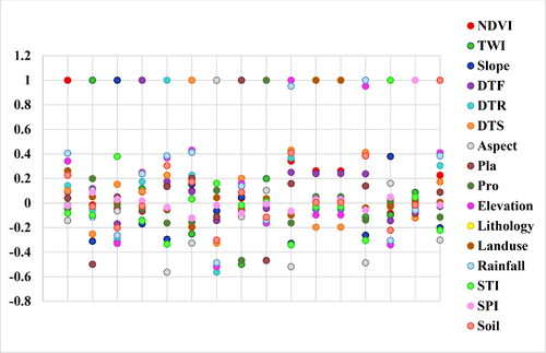
We analyzed, the correlation of each factor pair prior to modelling (Figure 8). The majority of correlations were below 0.2 while some exhibited values between 0.2 and 0.4, which means the factors were in low association and can be used for modelling. A high correlation was observed between precipitation and elevation as the precipitation changes with the elevation in the study area. The trace ratio criterion (TRC) could overcome this problem as optimal algorithm.

Figure 8. The relevance of landslide factor (DTF is distance to faults, DTR is distance to roads, DTS is distance to streams Pla is Plan Curvature, and Pro is profile curvature).

4.2. Application of models

4.2.1. MaxEnt

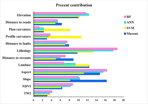
We constructed a MaxEnt model with the MaxEnt software (version 3.4.0) designed by Steven J. Phillips in Java. We compared the accuracy by adjusting the test and training samples, divisible mode, and other parameters. The maximum number of iterations was set as 500 to avoid over-fitting and weak fitting. Figure 9 depicts the comparative contributions of the environmental variables to the MaxEnt model. To ascertain the first valuation, the regularization gain increment was added to the contribution of the reciprocal variable in each iteration of the training algorithm or deducted if the absolute value changed to a negative value. In the second valuation, training variables and background data were randomly arranged for each environment variable (Pandey et al. 2020). Slope, aspect, and landuse were observed as the most important factors influencing landslide susceptibility.

Figure 9. The weight of every landslide sensitivity factor in Maxent, SVM, ANN and RF models.

4.2.2. SVM

The SVM model was built in Matlab (2020a, MathWorks) and required the input of both landslide and non-landslide pixels. Several landslide control factors were discrete objects and nonlinearly separable, thus we employed a sigmoid kernel to change the linearly non-separable samples into detachable linear samples. Not all samples needed to be paired, called a loss function. We assigned a relaxation factor (ξ) greater than or equal to 0 to induce a function interval greater than or equal to 1 then adding the relaxation factor (ξ). Denote C as a parameter controlling the weight of ξ, the smaller the value of C, the wider the transitional zone, and vice versa. More specifically, ξ can be regarded as a measure for the loss function. The loss function was causes by linear SVM allowing the existence of vectors in the transition band and compromises to some misclassified vectors (Pradhan 2013; Pandey et al. 2020). Figure 9 presents the SVM-determined factor contributions. Lithology, landuse, and aspect were identified as the most important factors influencing landslide susceptibility.

4.2.3. ANN

The ANN model was constructed in Matlab (2020a, MathWorks) with landslides and non-landslides pixel using memory-based learning. The input training and test data were employed to establish a memory model and the results were stored in a large memory source. Following the instruction of a new test vector, the learning process places the new vector into a stored class for classifications (Choi et al. 2012; Dou et al. 2015). Here 50% training data and 50% test data had been experimented but did not perform perfectly. Therefore, 30% and 70% of the test and training data were adopted, respectively. Figure 9 displays the contribution of each factor, with lithology, aspect, and elevation observed as the dominant factors impacting landslides.

4.2.4. Application of RF

RF was developed in Rstudio (version 3.4.1, RStudio) using the Random Forest extension. We defined ntree as 700 and mtry as 6 to obtain the optimal results. After 450 iterations the OOB (out of bag) curve achieved a perfect fit with a low stable error during modelling. Figure 9 depicts the conditional factor weights in the model to exhibit the weight of each conditional factor (Chen et al. 2018a). The Mean Decrease Accuracy is the OOB error, the Mean Decrease Gini is the purity of the subset after dependence partition. Slope, aspect, lithology, and elevation were more important so that it was significant to get a reasonable control of deviation (Youssef et al. 2016).

4.3. Landslide susceptibility mapping results

Figure 10 presents the landslide susceptibility maps determined via MaxEnt, SVM, ANN, and RF. The pixel values calculated using the models were used to generate classifications using the natural break classification scheme: low susceptibility (0.00-0.40), moderate susceptibility (0.40-0.70), high susceptibility (0.70-0.90), and very high susceptibility (0.90-1.00) (Pourghasemi et al. 2012; Chen et al. 2018b). The classification must abide by the following distribution: the majority of landslides occur in very high susceptible areas, several occur in high susceptible areas, and few landslides occur in low susceptible areas (Ayalew and Yamagishi 2005; Wang et al. 2019). Table 1 reports the classification results, landslide pixels, and FR values. The low susceptibility class was dominant, accounting for 40.52%, 52.22%, 50.63%, and 54.07% of the total for MaxEnt, SVM, ANN, and RF, and predicting 8.66%, 4.06%, 14.68%, and 2.76% of landslide pixels, respectively; the moderate group accounted for 30.96%, 27.48%, 28.11%, and 25.65% of the four models and predicted 17.29%, 9.77%, 12.70%, and 11.33% of the landslide pixels; the very high susceptibility class exhibited the lowest area: 9.86%, 8.21%, 6.90%, and 6.04%; and predicting the highest landslide pixels percentage at 52.19%, 62.83%, 51.81%, and 65.46%; the high susceptible group accounted for 18.66%, 12.09%, 14.35%, and 14.24%; and predicted 21.84%, 23.33%, 20.81%, and 20.46% of the landslide pixel percentages. The spatial distributions of the four maps followed similar trends.

Figure 10. Landslide susceptibility maps using (a) Maxent; (b) SVM; (c) ANN; (d) RF.

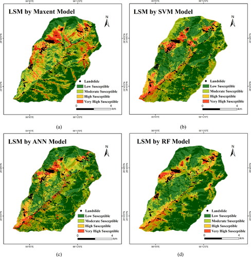
Table 1. Classification results and landslide pixels leading to corresponding FR values of the four models.

Susceptibility class	Number of pixels per class	Area in percentage (a)	Number of landslide pixels per class	Area in Percentage (b)	FR(b/a)
Maxent
VH	34983	9.86	2478	52.19	5.29
H	66205	18.66	1037	21.84	1.17
M	109851	30.96	821	17.29	0.56
L	143787	40.52	411	8.66	0.21
SVM
VH	29144	8.21	2983	62.83	7.65
H	42891	12.09	1108	23.33	1.93
M	97517	27.48	464	9.77	0.36
L	185274	52.22	193	4.06	0.08
ANN
VH	24495	6.90	2460	51.81	7.51
H	50924	14.35	988	20.81	1.45
M	99756	28.11	603	12.70	0.45
L	179651	50.63	697	14.68	0.29
RF
VH	21446	6.04	3008	63.35	10.84
H	51514	14.52	971	20.46	1.44
M	90015	25.37	538	11.33	0.44
L	191851	54.07	231	4.87	0.05

VH: Very high; H: High; M: Moderate; L: Low.

4.4. Model performance evaluation and validation

We employed map and mathematical verifications to evaluate and validate the study. The mathematical verification involves the testing of the model, including the ROC curve and RMSE (Pourghasemi and Rahmati 2018). Table 2 reports the comprehensive comparison.

Table 2. Comparison of the four models.

	Maxent	SVM	ANN	RF
RMSE	0.0347	0.0120	0.0999	0.0675
AUC (training/ validation dataset)	0.835 /0.807	0.909 /0.886	0.857 /0.844	0.885 /0.862
FR of VH	5.29	7.65	7.51	10.84

The rationality of each model classification is analyzed using the FR values in Table 1. The SVM is identified as the optimal model with the lowest additive value of VH and H susceptibility (20.30%) and the highest percentage of landslide pixels (86.16%) of the four models (Table 1). This is followed by RF, with the additive value of VH and H susceptibility determined as 20.56% and landslide pixels percentage of 83.81%. In addition, MaxEnt exhibited an additive value of VH and H susceptibility of 28.52% and landslide pixels percentage of 74.03%, while the corresponding values for ANN were 21.25% and 72.62%, respectively. All models exhibited reasonable distributions, while the SVM was optimal.

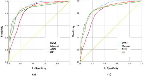
Machine learning (ML) methods generate a real value or probability prediction for a test sample and subsequently compare the predicted values with a classification threshold. A positive class is assigned if the prediction value is greater than the threshold, otherwise it will be classified as the inverse class. We changed the threshold from 0 to the maximum based on the prediction results of the learners. This allowed for each sample to be initially predicted as a positive example. As the threshold increased, the number of positive samples predicted was reduced by the learner until no sample was positive. The corresponding ROCs were obtained by calculating the values of two key variables and plotting their horizontal and vertical coordinates respectively. The ROC curve can easily identify the effect of any threshold on the generalized performance of the model (Youssef et al. 2016; Weidner et al. 2019). It can also select the optimal threshold; the nearer the ROC curve is to the upper left corner, the more precise the model. Our results demonstrate the best threshold close to the upper left corner, with the lowest total number of false positives and negatives and the fewest classification errors. We compared the model performance based on the ROC curves, in which the least distance from the upper left corner was associated with the highest accuracy. The AUC was introduced to identify the good and bad model points, however this proved to be difficult at the intersection of the two ROC curves (Mazzanti et al. 2020). The larger the AUC, the better the model performance is in many practical applications. Figure 11 presents the results of both the training and validation datasets via the four models. The AUC training curve, values were determined as 0.835 (83.5%), 0.909 (90.9%), 0.857 (85.7%), and 0.885 (88.5%), for MaxEnt, SVM, ANN, and RF respectively. The corresponding AUC validation curve values were 0.807 (80.7%), 0.886 (88.6%), 0.844 (84.4%), and 0.862 (86.2%), respectively. All models exhibited values greater than 0.75 and differences between training and validation data were less than 0.05. This implies the applicability of the LSM approaches in the study area. SVM was associated with the optimal training curve performance followed by RF, ANN, and MaxEnt. The same trend was observed for the validation curve. Table 2 reports the RMSE of the four models. SVM exhibiting the lowest value followed by MaxEnt, RF, and ANN.

Figure 11. ROC curves and AUC values using training dataset and validation dataset:(a)training dataset; (b) validation dataset.

4.5. Application of TRC-SVM

Despite the reasonable classification results of the four models in the study area, their performance is poor compared to other areas (with higher AUC values close to near 0.93 (93%)) (Pham et al. 2016; Hu et al. 2020). Therefore, we improve the optimal algorithm by fusing the TRC and SVM to obtain the TRC-SVM. In addition, the correlation between precipitation and elevation of all factors is very high, the TRC-SVM can improve the classification via the robust recombination and optimization of factors. Figure 12 depicts the LSM.

Figure 12. Landslide susceptibility map using TRC-SVM.

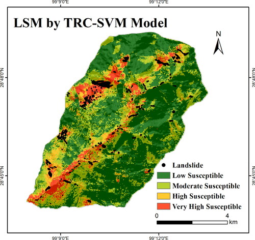
The TRC-SVM exhibits a flawless distribution of LSM around study area. The VH and H area is determined as 19.78% in total, with 85.41% landslide pixels and the RMSE remains unchanged. The AUC value is also improved (Figure 13), reaching 0.943 (94.3%) and 0.930 (93.0%) for the training and validation datasets, higher than the 0.909 (90.9%) and 0.886 (88.6%) SVM values, respectively (Table 3). The results reveal the higher accuracy of the optimized algorithm.

Figure 13. ROC curves and AUC values using training dataset and validation dataset:(a)training dataset; (b) validation dataset.

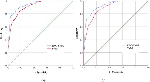
Table 3. Comparison of the SVM and TRC-SVM.

Susceptibility class	Number of pixels per class	Area in percentage (a)	Number of landslide pixels per class	Area in Percentage (b)	FR (b/a)	RSME	AUC (training/ validationdataset)
SVM						0.012	0.909/ 0.886
VH	29144	8.21	2983	62.83	7.65
H	42891	12.09	1108	23.33	1.93
M	97517	27.48	464	9.77	0.36
L	185274	52.22	193	4.06	0.08
TRC-SVM
VH	30081	8.48	3342	70.39	8.30	0.012	0.943/0.930
H	40097	11.30	713	15.02	1.33
M	96505	27.20	443	9.33	0.34
L	188143	53.02	250	5.27	0.09

5. Discussion

We initially employed 16 conditioning factors in the landslide susceptibility mapping (Dai and Lee 2003; Luo et al. 2019) and their contributions were analyzed prior to modelling (Vojteková and Vojtek 2020). The type of conditioning factors is so important that decides the precision of the susceptibility results.

Four models were compared: two linear (MaxEnt, SVM) and two nonlinear (ANN, RF) methods. These models are commonly used in landslide susceptibility assessments. RF was observed to outperform the ANN method in terms of the LSM for future landslides predictions in eastern Turkey (Sevgen et al. 2019). A study based in China revealed the ability of ANN to outperform SVM (Luo et al. 2019). However, the ANN is not always optimal. In Sari County, Iran, SVM exhibited better LSM classification results compared to the ANN (Kalantar et al. 2018). Moreover, a comparison of ANN SVM and MaxEnt demonstrated the latter to have a slight disadvantage (Chen et al. 2017). Numerous studies reveal the algorithm results to be a function of the sample classification, factor combinations, and even the research area, yet the underlying trend is the same. In the current study, determined the most suitable machine learning algorithm for LSM among the four models. Following multiple sample classifications and comprehensive factor selections, all models exhibited strong performances. However, the SVM achieved the highest AUC (0.909/0.886, training/validation dataset) and lowest RMSE (0.012), as well as reasonable FR values. The results indicate it to be the most suitable model for the study area. RF and ANN are on a par with MaxEnt based on just the evaluation method comparisons. (Table 2), with the following order in terms of RMSE: SVM, MaxEnt, RF and ANN. When AUC is used as the indicator, the models are ranked as SVM, RF, ANN and MaxEnt, and RF, SVM, ANN and MaxEnt when judging by FR values. In-depth investigations are not possible through the above comparison, thus we further employed field investigations and the analysis of landslide conditioning factors.

The pixel number of different LSM grades were compared with the number of pixels corresponding to the landslide (Table 1). This can also be regarded as a comparison of the FR under different LSM grades. It should be declining from VH to L that verified the models are in high reliability. However, the gradient of this ratio from VH to L can be further judging the models. Because H and M do not mean there is no landslide, it is reasonable H bigger than M and not very close with each other. So SVM is the best as its best gradient among them.

We then performed a detailed analysis of the factor performances in order to further explore the differences and similarities among the four models. As not all factors were of great significance, the most five influential factors selected for analysis. Table 4 reports the relationship between landslides, controlling factors, and the corresponding results of these factors and LSM determined from the four algorithms. Each factor was divided into several grades (classes) in order to determine the statistics of the following three variables: the proportion of each class in a factor; the number of landslide pixels in a class; and the domain of each level (very high susceptibility (VH), high susceptibility (H), moderate susceptibility (M) and low susceptibility (L)) for each model and class. The dominant conditioning factors were lithology, slope, aspect, elevation, and landuse. Figure 13 compares the detailed classification in VH of the five conditioning factors for the four models, where the pie represents the class proportion in VH and the height is the classification proportion in the conditioning factor (Figure 14) .

Figure 14. Detailed classification in VH of the top five conditioning factors for the four models.

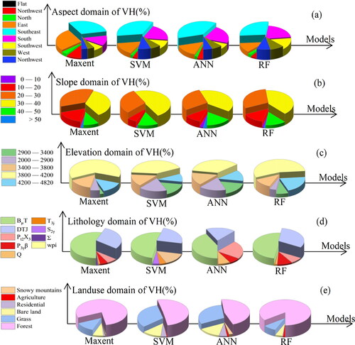
Table 4. Spatial relationship between landslides, conditional factors, and LSM.

Factors	Class	Class Domain (%)	Number of landslides pixels	Domain of VH/H/M/L(%)
				Maxent	SVM	ANN	RF
Aspect	Flat	0.22	2	0.0/0.1/0.2/0.4	0.1/0.5/0/0	0.0/0.1/0.2/0.3	0.0/0.2/0.2/0.3
	Northeast	2.38	46	9.7/2.9/1.6/0.8	3.3/3.2/3.8/0.9	3.8/2.9/1.4/2.7	3.9/3.3/2.5/2.0
	East	8.17	1070	28/11/5.2/3.9	15/12/8.6/6.0	15/11/8.2/7.1	12/12/7.9/7.5
	Southeast	21.04	1384	30/31/23/12	34/33/19/18	38/31/21/17	28/23/21/20
	South	14.33	887	12/15/17/12	20/19/14/12	22/19/15/12	21/13/12/14
	Southwest	12.61	403	7.2/11/15/13	11/11/13/13	7/12/15/12	15/14/10/13
	West	17.54	314	4.5/12/17/25	6.7/9.0/17/22	6.8/13/18/20	8.9/13/18/19
	Northwest	18.56	399	3.8/10/17/28	8.1/10/17/23	5.7/8.4/18/22	8.6/16/22/18
	North	5.15	243	4.0/5.2/4.9/5.5	1.6/2.2/7.0/5.2	1.7/2.1/3.8/7.0	2.3/4.7/5.9/5.1
Slope (angles)	0-10	3.80	107	0.3/0.8/1.3/7.7	0.3/2.0/6.5/2.9	2.1/2.2/3.5/4.0	1.1/3.0/3.6/4.3
	10-20	18.4	750	17/14/15/23	6.2/13.3/19/21	11/12/18/20	14/17/16/20
	20-30	35.51	1539	35/32/37/37	30/28/31/42	29/31/36/37	30/27/31/39
	30-40	31.98	1363	36/38/34/26	49/37/30/30	40/38/31/31	40/37/36/28
	40-50	9.01	826	10/13/11/5.5	13/17/11/4.7	16/14/9.3/7.1	13/15/11/6.7
	>50	1.29	163	1.6/1.9/1.7/0.6	0.7/2.7/2.4/0.2	2.3/2.4/1.4/0.9	1.1/1.8/1.6/2.0
Altitude (m)	2000-2900	9.19	368	2.6/8.4/11/9.7	16/23/13/1.9	17/20/11/5.6	7.7/12/17/5.1
	2900-3400	19.00	749	6.0/21/24/18	18/18/20/19	17/25/27/13	4.2/12/23/19
	3400-3800	25.50	630	15/24/31/26	15/20/23/30	16/22/26/28	12/25/25/27
	3800-4200	30.77	2034	63/37/26/22	42/31/29/30	36/26/28/32	55/43/30/27
	4200-4820	15.54	967	14/9.9/7.2/24	10/8.3/14/19	14/7.4/8.3/21	21/7.8/5.5/21
Lithology	BµT	28.73	2294	56/37/21/23	51/31/24/28	43/35/24/29	49/32/20/31
	DTJ	47.66	1558	30/40/45/58	24/38/46/55	19/28/51/52	31/45/50/49
	Pt2X3	5.68	522	6.6/7.1/8.3/2.6	15/14/5.1/2.3	23/12/3.9/3.0	7.9/7.8/8.0/3.9
	P3γβ	5.24	185	5.2/6.4/8.4/2.4	4.4/9.4/7.8/2.4	7.6/9.9/6.4/3.5	9.4/7.1/6.4/3.8
	Q	6.66	115	0.7/5.2/9.8/6.9	4.1/6.8/9.1/5.3	7.6/13/12/2.4	1.3/2.9/7.9/7.0
	T3j	3.63	69	0.4/1.9/4.7/4.7	0.4/0.6/4.5/4.3	0.3/0.9/2.0/5.7	0.7/4.3/6.5/2.4
	S2γ	0.69	0	0.2/0.3/0.2/1.3	0.0/0.1/0.9/0.8	0.2/0.1/0.3/1.2	0.0/0.7/0.3/1.0
	Σ	1.5	0	1.2/1.9/2.4/0.9	0.0/0.2/2.2/1.7	0.0/0.4/0.8/2.5	0.0/0.1/0.9/2.2
	wpi	0.16	0	0.0/0.0/0.2/0.3	0.0/0.0/0.2/0.2	0.0/0.2/0.1/0.3	0.0/0.0/0.0/0.3
Landuse	Snowy mountains	10.91	41	0.3/4.6/8.0/20	0.0/0.0/9.1/17	2.5/1.2/3.2/19	0.0/0.0/1.3/18
	Agriculture	2.81	282	0.2/0.6/1.0/1.0	0.5/0.9/1.5/0.3	1.2/1.3/1.1/5.1	1.3/2.1/1.6/0.2
	Residential	4.56	364	1.1/3.5/5.6/5.3	3.8/6.3/6.7/2.7	5.1/8.6/6.3/2.6	0.4/4.1/6.5/4.1
	Bare land	5.87	819	6.5/7.3/6.8/4.1	12/10/7.3/2.9	14/8.9/5.1/4.4	4.6/9.8/9.3/3.8
	Grass	26.33	1253	12/24/29/29	33/40/26/22	31/38/34/18	8.4/8.0/22/33
	Forest	49.53	1980	76/60/53/40	51/43/49/55	46/42/50/55	85/76/59/41

VH: Very high; H: High; M: Moderate; L: Low.

Previous research based on machine learning models determined aspect, slope and elevation as dominant factors impacting landslides (Nsengiyumva et al. 2019; Dou et al. 2020), particularly in XLG. Landslides to the southeast exhibited maximum VH levels across all models and were marked in red in Table 4. The 30-40 slope class accounted for the highest VH level, agreeing with the observations in the literature (Dahal 2014; Youssef et al. 2016). Our results also identified elevation as a significant factor in landslides, with a maximal duty ratio of 3,800-4,200 m for all four models at the VH level (Table 4) (Youssef et al. 2016; Cislaghi et al. 2019). B_µT exhibited the highest proportion of very high susceptible areas (nearly 50%) in all four models. However, a lower proportion area (28.73%) (red in Table 4) reveals B_µT to have the greatest influence on landslides in XLG. Moreover, the forest class was observed to be the dominant landuse (red in Table 4). Comparisons of the maximum percentage at the VH level for each class across all conditional factors indicate the high consistency and model was reliability.

Based on the strong correlation between the precipitation and elevation conditioning factors, we proposed several improvement measures. The four commonly used models achieved excellent susceptibility classification results, however the improved synthesis algorithms exhibited a better performance (Saha et al. 2020; Zhao and Zhao 2021). This study improved the optimal algorithm of the four models through two key steps: (1) the high correlation between precipitation and elevation allowed precipitation to be ignored in the factor refinement classification. However, precipitation was identified as an important LSM factor (Bui et al. 2015) and thus it could not be ignored in modelling. The TRC algorithm was thus introduced into the optimal model (SVM) as the TRC-SVM. Despite no improvements in the RMSE (0.012), the TRC-SVM increased the classification accuracy and maintained stability. (2) The proposed model enhanced the AUC values from 0.886 to 0.930 for the validation dataset and from 0.909 to 0.943 for the training dataset. Comparisons of the FR values reveal the slight superiority of the TRC-SVM compared to SVM in VH, while this was not the case for the gradient. The improved algorithm thus exhibited a better classification effect for the XLG.

6. Conclusions

Landslide susceptibility mapping is of great significance in large-scale landslide prediction and is used with increasing frequency in areas where it is difficult to conduct a full field investigation (e.g., southwest China). In the current study, we conducted landslide susceptibility mapping based on four machine learning methods, namely two linear (MaxEnt and SVM) and two nonlinear (ANN and RF) algorithms that are representative approaches for landslide susceptibility mapping. Following a comprehensive review of the literature, 16 conditional factors were summarized and calculated via the four models. We aimed to comprehensively select the most suitable susceptibility evaluation model for XLG and similar areas. The AUC was slightly lower than some of the other studies, although the models were consistent. Thus, the optimal SVM algorithm was improved with the proposed TRC-SVM, enhancing the classification results. This algorithm can be applied to similar mountainous areas to for susceptibility zoning. These results also provide an effective basis for government decision-making and urban planning for disaster prevention and mitigation, as well as resident relocation, due to landslides in southwest China.

All models employed 16 factors in order to reflect the fairness of the four models, there is no classification analysis for which factors are suitable for certain model. The factor combinations may affect the modelling process. This is a disadvantage of the SVM and may be overcome by integrating the TRC algorithm with ANN, RF or MaxEnt. The investigation of such problems is reserved for future work. Our work demonstrates the ability of the TRC to optimize machine learning classification to some extent, making a contribution to the factor optimization of the SVM algorithm.

Acknowledgements

This work was financially supported by the National Key Research and Development Program of China [grant number: 2017YFC1501004], the National Natural Science Foundation of China [grant number: 41807227; 42022053; U1702241; 41877220]. We thank the editor and anonymous reviewers for improving the original manuscript. We would like to express deep and sincere gratitude to Prof. Dr. Chen Cao, who has taught and guided us in research.

Disclosure statement

No potential conflict of interest was reported by the authors.

Data availability statement

Not applicable.

Additional information

Funding

This work was supported by the National Key Research and Development Program of China [grant number: 2017YFC1501004], the National Natural Science Foundation of China [grant number: 41807227; 42022053; U1702241;41877220].

References

- Arabameri A, Asadi Nalivan O, Chandra Pal S, Chakrabortty R, Saha A, Lee S, Pradhan B, Bui DT. 2020. Novel machine learning approaches for modelling the gully erosion susceptibility. Remote Sens. 12(17):2833.
- Arabameri A, Pradhan B, Rezaei K, Sohrabi M, Kalantari Z. 2019. GIS-based landslide susceptibility mapping using numerical risk factor bivariate model and its ensemble with linear multivariate regression and boosted regression tree algorithms. J Mt Sci. 16(3):595–618. https://doi.org/http://dx.doi.org/10.1007/s11629-018-5168-y.
- Ayalew L, Yamagishi H. 2005. The application of GIS-based logistic regression for landslide susceptibility mapping in the Kakuda-Yahiko Mountains, Central Japan. Geomorphology. 65(1-2):15–31.
- Azareh A, Rahmati O, Rafiei-Sardooi E, Sankey JB, Lee S, Shahabi H, Ahmad BB. 2019. Modelling gully-erosion susceptibility in a semi-arid region, Iran: Investigation of applicability of certainty factor and maximum entropy models. Sci Total Environ. 655:684–696.
- Babb T, Bliss L. 1974. Susceptibility to environmental impact in the Queen Elizabeth Islands. Arctic. 27(3):234–237. https://doi.org/http://dx.doi.org/10.14430/arctic2877.
- Bai S, Wang J, Zhang Z, Cheng C. 2012. Combined landslide susceptibility mapping after Wenchuan earthquake at the Zhouqu segment in the Bailongjiang Basin, China. Catena. 99:18–25.
- Booth JS, Silva AJ, Jordan SA. 1984. Slope-stability analysis and creep susceptibility of Quaternary sediments on the northeastern United States continental slope. In Seabed mechanics. Springer, Berlin, Germany, p. 65–75.
- Bui DT, Pradhan B, Revhaug I, Nguyen DB, Pham HV, Bui QN. 2015. A novel hybrid evidential belief function-based fuzzy logic model in spatial prediction of rainfall-induced shallow landslides in the Lang Son city area (Vietnam). Geomatics Nat Hazards Risk. 6(3):243–271.
- Bui DT, Tuan TA, Klempe H, Pradhan B, Revhaug I. 2016. Spatial prediction models for shallow landslide hazards: a comparative assessment of the efficacy of support vector machines, artificial neural networks, kernel logistic regression, and logistic model tree. Landslides. 13(2):361–378. https://doi.org/http://dx.doi.org/10.1007/s10346-015-0557-6.
- Cama M, Schillaci C, Kropáček J, Hochschild V, Bosino A, Märker M. 2020. A probabilistic assessment of soil erosion susceptibility in a head catchment of the Jemma Basin, Ethiopian Highlands. Geosciences. 10(7):248.
- Cao C, Chen J, Zhang W, Xu P, Zheng L, Zhu C. 2019. Geospatial analysis of mass-wasting susceptibility of four small catchments in mountainous area of Miyun County. IJERPH. 16(15):2801.
- Chang Z, Du Z, Zhang F, Huang F, Chen J, Li W, Guo Z. 2020. Landslide susceptibility prediction based on remote sensing images and GIS: Comparisons of supervised and unsupervised machine learning models. Remote Sens. 12(3):502.
- Chen W, Chen Y, Tsangaratos P, Ilia I, Wang X. 2020. Combining evolutionary algorithms and machine learning models in landslide susceptibility assessments. Remote Sens. 12(23):3854.
- Chen W, Peng J, Hong H, Shahabi H, Pradhan B, Liu J, Zhu A-X, Pei X, Duan Z. 2018a. Landslide susceptibility modelling using GIS-based machine learning techniques for Chongren County, Jiangxi Province, China. Sci Total Environ. 626:1121–1135.
- Chen W, Pourghasemi HR, Kornejady A, Zhang N. 2017. Landslide spatial modeling: introducing new ensembles of ANN, MaxEnt, and SVM machine learning techniques. Geoderma. 305:314–327.
- Chen W, Zhang S, Li R, Shahabi H. 2018b. Performance evaluation of the GIS-based data mining techniques of best-first decision tree, random forest, and naïve Bayes tree for landslide susceptibility modeling. Sci Total Environ. 644:1006–1018.
- Choi J, Oh H-J, Lee H-J, Lee C, Lee S. 2012. Combining landslide susceptibility maps obtained from frequency ratio, logistic regression, and artificial neural network models using ASTER images and GIS. Eng Geol. 124:12–23.
- Cislaghi A, Giupponi L, Tamburini A, Giorgi A, Bischetti GB. 2019. The effects of mountain grazing abandonment on plant community, forage value and soil properties: observations and field measurements in an alpine area. Catena. 181:104086.
- Dahal RK. 2014. Regional-scale landslide activity and landslide susceptibility zonation in the Nepal Himalaya. Environ Earth Sci. 71(12):5145–5164. https://doi.org/http://dx.doi.org/10.1007/s12665-013-2917-7.
- Dai F, Lee C. 2003. A spatiotemporal probabilistic modelling of storm‐induced shallow landsliding using aerial photographs and logistic regression. Earth Surf Process Landforms. 28(5):527–545.
- De Ploey J, Moeyersons J, Goossens D. 1995. The De Ploey erosional susceptibility model for catchments, ES. Catena. 25(1-4):269–314.
- Dou J, Yamagishi H, Pourghasemi HR, Yunus AP, Song X, Xu Y, Zhu Z. 2015. An integrated artificial neural network model for the landslide susceptibility assessment of Osado Island. Nat Hazards. 78(3):1749–1776. https://doi.org/http://dx.doi.org/10.1007/s11069-015-1799-2.
- Dou J, Yunus AP, Merghadi A, Shirzadi A, Nguyen H, Hussain Y, Avtar R, Chen Y, Pham BT, Yamagishi H. 2020. Different sampling strategies for predicting landslide susceptibilities are deemed less consequential with deep learning. Sci Total Environ. 720:137320.
- Fang Z, Wang Y, Peng L, Hong H. 2020. Integration of convolutional neural network and conventional machine learning classifiers for landslide susceptibility mapping. Comput Geosci. 139:104470.
- Godone D, Allasia P, Borrelli L, Gullà G. 2020. UAV and structure from motion approach to monitor the Maierato landslide evolution. Remote Sens. 12(6):1039.
- Goetz J, Brenning A, Petschko H, Leopold P. 2015. Evaluating machine learning and statistical prediction techniques for landslide susceptibility modeling. Comput Geosci. 81:1–11. https://doi.org/http://dx.doi.org/10.1016/j.cageo.2015.04.007.
- Gorum T, van Westen CJ, Korup O, van der Meijde M, Fan X, van der Meer FD. 2013. Complex rupture mechanism and topography control symmetry of mass-wasting pattern, 2010 Haiti earthquake. Geomorphology. 184:127–138.
- Hong H, Liu J, Bui DT, Pradhan B, Acharya TD, Pham BT, Zhu A-X, Chen W, Ahmad BB. 2018. Landslide susceptibility mapping using J48 decision tree with AdaBoost, bagging and rotation forest ensembles in the Guangchang area (China). Catena. 163:399–413.
- Hu Q, Zhou Y, Wang S, Wang F. 2020. Machine learning and fractal theory models for landslide susceptibility mapping: Case study from the Jinsha River Basin. Geomorphology. 351:106975.
- Huang F, Cao Z, Guo J, Jiang S-H, Li S, Guo Z. 2020. Comparisons of heuristic, general statistical and machine learning models for landslide susceptibility prediction and mapping. Catena. 191:104580.
- Jiang Y, Xu Q, Lu Z, Luo H, Liao L, Dong X. 2021. Modelling and predicting landslide displacements and uncertainties by multiple machine-learning algorithms: application to Baishuihe landslide in Three Gorges Reservoir, China. Geomatics Nat Hazards Risk. 12(1):741–762.
- Jibson RW, Keefer DK. 1989. Statistical analysis of factors affecting landslide distribution in the New Madrid seismic zone, Tennessee and Kentucky. Eng Geol. 27(1-4):509–542.
- Jones J, Boulton S, Bennett G, Whitworth M, Stokes M. 2020. Himalaya mass-wasting: impacts of the monsoon, extreme tectonic and climatic forcing, and road construction. In EGU General Assembly Conference Abstracts, 8702.
- Kalantar B, Pradhan B, Naghibi SA, Motevalli A, Mansor S. 2018. Assessment of the effects of training data selection on the landslide susceptibility mapping: a comparison between support vector machine (SVM), logistic regression (LR) and artificial neural networks (ANN). Geomatics Nat Hazards Risk. 9(1):49–69.
- Kariminejad N, Hosseinalizadeh M, Pourghasemi HR, Bernatek-Jakiel A, Campetella G, Ownegh M. 2019. Evaluation of factors affecting gully headcut location using summary statistics and the maximum entropy model: Golestan Province, NE Iran. Sci Total Environ. 677:281–298.
- Khamkar DJ, Mhaske SY. 2019. Identification of landslide susceptible settlements using geographical information system of Yelwandi river basin, Maharashtra (India). Nat Hazards. 96(3):1263–1287. https://doi.org/http://dx.doi.org/10.1007/s11069-019-03609-0.
- Kornejady A, Ownegh M, Bahremand A. 2017. Landslide susceptibility assessment using maximum entropy model with two different data sampling methods. Catena. 152:144–162.
- Li Z, Nie F, Chang X, Yang Y. 2017. Beyond trace ratio: weighted harmonic mean of trace ratios for multiclass discriminant analysis. IEEE Trans Knowl Data Eng. 29(10):2100–2110.
- Li S, Wu L, Chen J, Huang R. 2020. Multiple data-driven approach for predicting landslide deformation. Landslides. 17(3):709–718. https://doi.org/http://dx.doi.org/10.1007/s10346-019-01320-6.
- Luo X, Lin F, Zhu S, Yu M, Zhang Z, Meng L, Peng J. 2019. Mine landslide susceptibility assessment using IVM, ANN and SVM models considering the contribution of affecting factors. Plos One. 14(4):e0215134.
- Maloney JM, Bentley SJ, Xu K, Obelcz J, Georgiou IY, Jafari NH, Miner MD. 2020. Mass wasting on the Mississippi River subaqueous delta. Earth Sci Rev. 200:103001.
- Marjanović M. 2013. Comparing the performance of different landslide susceptibility models in ROC space. In Landslide science and practice. Springer, Berlin, Heidelberg; p. 579–584.
- Mazzanti P, Caporossi P, Muzi R. 2020. Sliding time master digital image correlation analyses of cubesat images for landslide monitoring: the Rattlesnake Hills landslide (USA). Remote Sens. 12(4):592. https://doi.org/http://dx.doi.org/10.3390/rs12040592.
- Moayedi H, Mehrabi M, Mosallanezhad M, Rashid ASA, Pradhan B. 2019. Modification of landslide susceptibility mapping using optimized PSO-ANN technique. Eng Comput. 35(3):967–984. https://doi.org/http://dx.doi.org/10.1007/s00366-018-0644-0.
- Nhu V-H, Hoang N-D, Nguyen H, Ngo PTT, Bui TT, Hoa PV, Samui P, Bui DT. 2020. Effectiveness assessment of keras based deep learning with different robust optimization algorithms for shallow landslide susceptibility mapping at tropical area. Catena. 188:104458. https://doi.org/http://dx.doi.org/10.1016/j.catena.2020.104458.
- Nsengiyumva JB, Luo G, Amanambu AC, Mind'je R, Habiyaremye G, Karamage F, Ochege FU, Mupenzi C. 2019. Comparing probabilistic and statistical methods in landslide susceptibility modeling in Rwanda/Centre-Eastern Africa. Sci Total Environ. 659:1457–1472.
- Nsengiyumva JB, Valentino R. 2020. Predicting landslide susceptibility and risks using GIS-based machine learning simulations, case of upper Nyabarongo catchment. Geomatics Nat Hazards Risk. 11(1):1250–1277.
- Pandey VK, Pourghasemi HR, Sharma MC. 2020. Landslide susceptibility mapping using maximum entropy and support vector machine models along the Highway Corridor, Garhwal Himalaya. Geocarto Int. 35(2):168–187. https://doi.org/http://dx.doi.org/10.1080/10106049.2018.1510038.
- Pannatier A, Oppikofer T, Jaboyedoff M, Stock G. 2009. Rockfall susceptibility mapping of Yosemite Valley (USA) using a high-resolution digital elevation model. EGUGA. 7692
- Parker RN, Densmore AL, Rosser NJ, De Michele M, Li Y, Huang R, Whadcoat S, Petley DN. 2011. Mass wasting triggered by the 2008 Wenchuan earthquake is greater than orogenic growth. Nature Geosci. 4(7):449–452. https://doi.org/http://dx.doi.org/10.1038/ngeo1154.
- Peethambaran B, Anbalagan R, Kanungo D, Goswami A, Shihabudheen K. 2020. A comparative evaluation of supervised machine learning algorithms for township level landslide susceptibility zonation in parts of Indian Himalayas. Catena. 195:104751. https://doi.org/http://dx.doi.org/10.1016/j.catena.2020.104751.
- Pham BT, Pradhan B, Bui DT, Prakash I, Dholakia M. 2016. A comparative study of different machine learning methods for landslide susceptibility assessment: a case study of Uttarakhand area (India). Environ Model Software. 84:240–250.
- Polykretis C, Chalkias C, Ferentinou M. 2019. Adaptive neuro-fuzzy inference system (ANFIS) modeling for landslide susceptibility assessment in a Mediterranean hilly area. Bull Eng Geol Environ. 78(2):1173–1187. https://doi.org/http://dx.doi.org/10.1007/s10064-017-1125-1.
- Pourghasemi HR, Mohammady M, Pradhan B. 2012. Landslide susceptibility mapping using index of entropy and conditional probability models in GIS: Safarood Basin, Iran. Catena. 97:71–84.
- Pourghasemi HR, Rahmati O. 2018. Prediction of the landslide susceptibility: Which algorithm, which precision? Catena. 162:177–192.
- Pradhan B. 2013. A comparative study on the predictive ability of the decision tree, support vector machine and neuro-fuzzy models in landslide susceptibility mapping using GIS. Comput Geosci. 51:350–365.
- Prasad AS, Pandey BW, Leimgruber W, Kunwar RM. 2016. Mountain hazard susceptibility and livelihood security in the upper catchment area of the river Beas, Kullu Valley, Himachal Pradesh. Geoenviron Disasters. 3(1):3.
- Roth RA. 1983. Factors affecting landslide-susceptibility in San Mateo county, California. Bull Assoc Eng Geol. xx(4):353–372.
- Saha AK, Gupta RP, Sarkar I, Arora MK, Csaplovics E. 2005. An approach for GIS-based statistical landslide susceptibility zonation—with a case study in the Himalayas. Landslides. 2(1):61–69. https://doi.org/http://dx.doi.org/10.1007/s10346-004-0039-8.
- Saha S, Saha A, Hembram TK, Pradhan B, Alamri AM. 2020. Evaluating the performance of individual and novel ensemble of machine learning and statistical models for landslide susceptibility assessment at Rudraprayag District of Garhwal Himalaya. Appl Sci. 10(11):3772. https://doi.org/http://dx.doi.org/10.3390/app10113772.
- Salles T, Duclaux G. 2015. Combined hillslope diffusion and sediment transport simulation applied to landscape dynamics modelling. Earth Surf Process Landforms. 40(6):823–839.
- Sevgen E, Kocaman S, Nefeslioglu HA, Gokceoglu C. 2019. A novel performance assessment approach using photogrammetric techniques for landslide susceptibility mapping with logistic regression, ANN and random forest. Sensors. 19:3940.
- Sun D, Wen H, Wang D, Xu J. 2020. A random forest model of landslide susceptibility mapping based on hyperparameter optimization using Bayes algorithm. Geomorphology. 362:107201. https://doi.org/http://dx.doi.org/10.1016/j.geomorph.2020.107201.
- Tehrani FS, Santinelli G, Herrera MH. 2021. Multi-Regional landslide detection using combined unsupervised and supervised machine learning. Geomatics Nat Hazards Risk. 12(1):1015–1038.
- Tian Y, Xu C, Hong H, Zhou Q, Wang D. 2019. Mapping earthquake-triggered landslide susceptibility by use of artificial neural network (ANN) models: an example of the 2013 Minxian (China) Mw 5.9 event. Geomatics Nat Hazards Risk. 10(1):1–25.
- Tonini M, D’Andrea M, Biondi G, Degli Esposti S, Trucchia A, Fiorucci P. 2020. A machine learning-based approach for wildfire susceptibility mapping. The case study of the Liguria region in Italy. Geosciences. 10(3):105. https://doi.org/http://dx.doi.org/10.3390/geosciences10030105.
- Vakhshoori V, Zare M. 2018. Is the ROC curve a reliable tool to compare the validity of landslide susceptibility maps? Geomatics Nat Hazards Risk. 9(1):249–266.
- Vasu NN, Lee S-R. 2016. A hybrid feature selection algorithm integrating an extreme learning machine for landslide susceptibility modeling of Mt. Woomyeon, South Korea. Geomorphology. 263:50–70.
- Vojteková J, Vojtek M. 2020. Assessment of landslide susceptibility at a local spatial scale applying the multi-criteria analysis and GIS: a case study from Slovakia. Geomatics Nat Hazards Risk. 11(1):131–148. https://doi.org/http://dx.doi.org/10.1080/19475705.2020.1713233.
- Wang S, Ding Z, Fu Y. 2017. Feature selection guided auto-encoder. In Proceedings of the AAAI Conference on Artificial Intelligence.
- Wang Y, Fang Z, Hong H. 2019. Comparison of convolutional neural networks for landslide susceptibility mapping in Yanshan County, China. Sci Total Environ. 666:975–993.
- Weidner L, DePrekel K, Oommen T, Vitton S. 2019. Investigating large landslides along a river valley using combined physical, statistical, and hydrologic modeling. Eng Geol. 259:105169.
- Wiesmair M, Otte A, Waldhardt R. 2017. Relationships between plant diversity, vegetation cover, and site conditions: implications for grassland conservation in the Greater Caucasus. Biodivers Conserv. 26(2):273–291. https://doi.org/http://dx.doi.org/10.1007/s10531-016-1240-5.
- Xu T, Xu Q, Deng M, Ma T, Yang T, Tang C-a. 2014. A numerical analysis of rock creep-induced slide: a case study from Jiweishan Mountain. Environ Earth Sci. 72(6):2111–2128.
- Youssef AM, Pourghasemi HR, Pourtaghi ZS, Al-Katheeri MM. 2016. Landslide susceptibility mapping using random forest, boosted regression tree, classification and regression tree, and general linear models and comparison of their performance at Wadi Tayyah Basin, Asir Region, Saudi Arabia. Landslides. 13(5):839–856. https://doi.org/http://dx.doi.org/10.1007/s10346-015-0667-1.
- Yuan Y, Xu T, Heap MJ, Meredith PG, Yang T, Zhou G. 2021. A three-dimensional mesoscale model for progressive time-dependent deformation and fracturing of brittle rock with application to slope stability. Comput Geotech. 135:104160.
- Zhang K, Wu X, Niu R, Yang K, Zhao L. 2017. The assessment of landslide susceptibility mapping using random forest and decision tree methods in the Three Gorges Reservoir area. Environ Earth Sci. 76(11):1–20. https://doi.org/http://dx.doi.org/10.1007/s12665-017-6731-5.
- Zhao S, Zhao Z. 2021. A comparative study of landslide susceptibility mapping using SVM and PSO-SVM models based on grid and slope units. Math Prob Eng. 2021:1–15.
- Zhu G, Blumberg DG. 2002. Classification using ASTER data and SVM algorithms: The case study of Beer Sheva, Israel. Remote Sens Environ. 80(2):233–240.