Gene expression programming and ensemble methods for bushfire susceptibility mapping: a case study of Victoria, Australia

Abstract

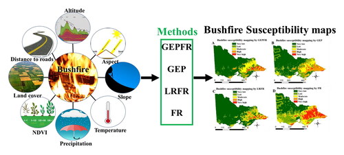
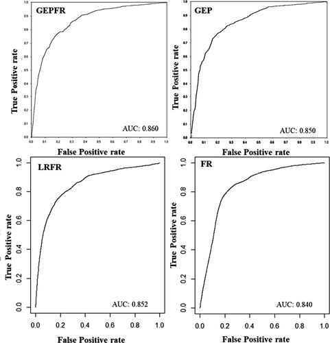
Bushfire susceptibility mapping helps the government authorities predict and provide the required disaster management plans to reduce the adverse impacts from bushfires. In this paper, we investigated Gene Expression Programming (GEP) and ensemble methods to create bushfire susceptibility maps for Victoria, Australia, as a case study. Bushfire susceptibility maps indicate that the eastern part of Victoria where forests are predominant has the highest probability of bushfire. Western part of Victoria which is covered by cropland, shrubland and grassland has the lowest bushfire probability. Two ensemble methods, namely an ensemble of GEP and Frequency Ratio (GEPFR) and an ensemble of Logistic Regression and Frequency Ratio (LRFR), were proposed and compared with stand-alone GEP and stand-alone Frequency Ratio (FR) methods. The proposed methods were evaluated by Area Under Curve (AUC). AUCs of GEPFR, LRFR, GEP and FR are 0.860, 0.852, 0.850, and 0.840, respectively. It can be concluded that GEPFR outperforms the other three methods, and the ensemble methods outperform the stand-alone methods. GEPFR, LRFR and GEP produced the bushfire probability with an accuracy in the range of 90.79%−92.27%, and therefore they are equally useful for policy makers and managers to have better natural hazard management plans.

Graphical Abstract

Keywords:

• Bushfire
• GEP
• susceptibility map
• natural hazard
• GIS

1. Introduction

Bushfires harm human life and have destructive consequences in the environment, especially in the populated areas (Tonini et al. 2020). The number and severity of bushfires have been increased in many parts of the world during the last decade due to the global warming, industrialization and human activities (Ghorbanzadeh et al. 2018; Zhang et al. 2019; Gholamnia et al. 2020). In one bushfire season alone, from late 2019 to early 2020, more than 12.6 million ha across Australia were burned, and as a result, 434 million tons of carbon dioxide were emitted (Werner and Lyons 2020). The bushfire season in 2019–2020 resulted in the loss of 33 people and over one billion animals across Australia (Werner and Lyons 2020). Southeastern Australia was the most affected area. Twenty four casualties with around 5 million ha of the burned areas belong to Southeastern Australia (Green et al. 2020), while over one million ha was burned in Victoria (Bunch 2020).

A bushfire susceptibility model could be a valuable tool to control and manage the future bushfires by predicting the vulnerable areas. Important factors in bushfire occurrence can be divided into four main categories including topography, climate, fuel loads and human activities (Hong et al. 2019; Jaafari and Pourghasemi 2019). Topographic factors such as elevation, slope, and aspect play an important role in bushfires (Tolhurst et al. 2008; O’Connor et al. 2016; Clarke et al. 2019). Many scholars have used a variety of climatic conditioning factors such as temperature (Tehrany et al. 2019; Zhang et al. 2019; Pham et al. 2020), precipitation (Jaafari et al. 2017; Zhang et al. 2019), wind speed (Jaafari et al. 2017; Tehrany et al. 2019), and humidity (Tehrany et al. 2019). Fuel loads are another conditioning factor that can be grouped into two subcategories, namely Normalized Difference Vegetation Index (NDVI) (Tehrany et al. 2019; Zhang et al. 2019), and land use/land cover (De Vasconcelos et al. 2001; Jaafari et al. 2017; Pham et al. 2020; Shang et al. 2020). The previous research on bushfires also used different human activity factors such as distance to roads (De Vasconcelos et al. 2001; Jaafari et al. 2017; Valdez et al. 2017; Jaafari et al. 2018; Pham et al. 2020), distance to populated areas (Jaafari et al. 2017; You et al. 2017; Hong et al. 2019) and distance to rivers (Valdez et al. 2017; Jaafari et al. 2017; Jaafari et al. 2018; Jaafari et al. 2019c; Zhang et al. 2019). The abovementioned four factors are closely related to the bushfire occurrence. Topography is one of the main drivers of bushfires because slope influences the spread rate of bushfires (Leonard and Blanchi 2012). Fire can move faster upslope and slower downslope (Leonard and Blanchi 2012). Topography can also affect the distribution of vegetation, climate elements (e.g. wind speeds), temperature, precipitation, and solar radiation (Tien Bui et al. 2016; Leuenberger et al. 2018; Eskandari et al. 2020a). Meteorological parameters such as temperature were reported as a significant factor in bushfire prediction (Ghorbanzadeh et al. 2019b). Temperature has a direct relationship with fire occurrence (Ghorbanzadeh et al. 2019b). The chance of bushfire is higher in places and times with a higher temperature (Nicholls and Lucas 2007). NDVI plays an important role in bushfire modelling (Tien Bui et al. 2016; Zhang et al. 2016). Different types of vegetation were considered as a proxy of fuel, and NDVI was used to explain the vegetation status (Tien Bui et al. 2016). Low NDVI indicates water stress, hence increases the risk of fire (Ghorbanzadeh et al. 2019b). Fire can quickly spread in highly connected forest patches, whereas patches of irregular shapes reduce the spread rate of fire (Gralewicz et al. 2012). Bushfire occurrence is more probable in the areas near human activities (Zhang et al. 2015). As a result, distance to roads and human facilities were reported to be negatively correlated with bushfire occurrence (Zhang et al. 2015).

Different statistical approaches have been used for bushfire susceptibility mapping including Frequency Ratio (FR) (Dorji and Ongsomwang 2017; Hong et al. 2017), Evidential Belief Function (EBF) (Pourghasemi 2016), and Weight Of Evidence (WOE) (Jaafari et al. 2017; Hong et al. 2019). Significant advances have been made in bushfire monitoring by remote-sensing technologies. The improvement in the quality of weather data and a sufficient amount of remotely sensed data has created an opportunity for scientists to use a data-driven approach to bushfire modelling (Jain et al. 2020). As a result, Machine Learning (ML) techniques have been used increasingly in bushfire management (Jain et al. 2020). ML includes a class of algorithms that produce susceptibility maps based on input data without the need for prior knowledge. ML learns from experience, and once the model is fitted, it will generate bushfire susceptibility maps for the whole study area (Leuenberger et al. 2018; Tonini et al. 2020).

Different ML approaches have been applied to bushfire susceptibility mapping. The previous research used Random Forest (RF) (Sachdeva et al. 2018; Jaafari and Pourghasemi 2019; Ghorbanzadeh et al. 2019b; Tonini et al. 2020; Eskandari et al. 2020b), Adaptive Neuro Fuzzy Interface System (ANFIS) (Jaafari et al. 2019a, 2019b; Moayedi et al. 2020; Razavi-Termeh et al. 2020), Support Vector Machines (SVM) (Tien Bui et al. 2017; Sachdeva et al. 2018; Jaafari and Pourghasemi 2019; Ghorbanzadeh et al. 2019b), Logistic Regression (LR) (Catry et al. 2009; Pourghasemi 2016; Dorji and Ongsomwang 2017; Sachdeva et al. 2018; Jaafari et al. 2019c), and Artificial Neural Networks (ANN) (Sachdeva et al. 2018; Ghorbanzadeh et al. 2019a).

Gene expression programming (GEP) is a branch of artificial intelligence methods that can automatically find the explicit function between dependent and independent variables without any assumption on the function form (Emamgolizadeh et al. 2015; Hoang and Tien Bui 2018). GEP can find the nonlinear relationship between a response variable and conditioning factors (Emamgolizadeh et al. 2015). GEP is proven to be an effective method for predicting natural hazards such as landslides and other engineering fields (Zakaria et al. 2010; Kayadelen 2011; Emamgolizadeh et al. 2015). The GEP algorithm is proven to be a promising tool for the prediction of shallow landslides in Son La Province, Vietnam (Hoang and Tien Bui 2018). GEP was also used in other engineering fields such as high-performance concrete (HPC) to formulate compressive strength of HPC mixes (Mousavi et al. 2012). However, to the best of our knowledge, GEP has not been explored in bushfire studies. Therefore, the overarching aim of this paper is to investigate the potential of GEP for bushfire susceptibility mapping. In this paper, we proposed four methods, namely an ensemble of GEP and FR (GEPFR), a single GEP, an ensemble of LR and FR (LRFR), and a single FR to create bushfire susceptibility maps for Victoria, Australia, as a case study. For this purpose, we collected necessary data for conditioning factors in Victoria. Then, we had generated the required conditioning factor maps that were later used for generating the bushfire susceptibility maps, as explained in the materials and method section. Then, the generated models were validated and compared in the result and discussion section. The methods used in this research are generic and scalable, hence they can be applied to other bushfire-prone countries.

2. Materials and methods

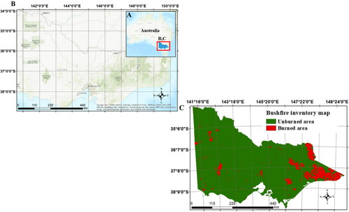
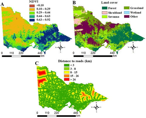
This study aims to investigate the bushfire susceptibility in Victoria located in Southeastern Australia, between latitudes from 34˚ S to 39˚ S and longitudes from 141˚ E to 150˚ E with an area of 227,444 km² (Figure 1). New South Wales occupies the northern side, and South Australia is located on the western side of Victoria. Victoria is surrounded by Tasman Sea and the Indian (southern) Ocean on the south. Plant cover in Victoria includes forests, savannas and grasslands.

Figure 1. Map of the study area: (A) map of Australia and the location of Victoria, (B) Map of Victoria in more details and (C) a bushfire inventory map for Victoria. Red colour represents burned areas and green shows unburned areas.

2.2. Data collection

2.2.1. Fire data

Collecting data is a fundamental step prior to the generation of bushfire susceptibility mapping (Eskandari et al. 2020a). In this study, the history of bushfires in Victoria was collected from the MODIS fire product (MODIS 500-m MCD 64 Monthly) from the NASA website for the period of fire seasons between 2010 and 2020. The burned areas were classified as 1 and unburned areas were classified as 0 in inventory map of our study area (Figure 1C). Fire seasons in Australia occur from November to February. The MODIS data will help researchers generate inventory maps that are important sources of information for elaborating hazard, risk and susceptibility maps (Tonini et al. 2020). This data can be found at http://modis-fire.umd.edu.

2.2.2. Effective factors on bushfires

Bushfires are a complex phenomenon, and many factors are involved in bushfire occurrence. There is no definite answer to which factor plays the most important role for the prediction of bushfires (Hong et al. 2019). As a result, we consider the following four factors in our study based on the literature (Jaafari et al. 2017; You et al. 2017; Sachdeva et al. 2018; Hong et al. 2019; Zhang et al. 2019; Jaafari et al. 2019c; Tonini et al. 2020; Eskandari et al. 2020a), and the availability of the data: topography, climate, fuel loads, and human-made factors. Topographical factors include slope, aspect, and digital elevation models. Climatic factors are mainly annual mean precipitation and annual mean temperature. Fuel loads and human-made factors include NDVI, land cover, and distance to roads.

2.2.2.1. Topographic factors

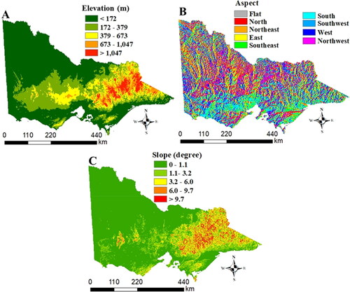
A Digital Elevation Model (DEM) known as ASTER 30-m GDEM (Figure 2A) was provided by the United States Geological Survey (USGS) (USGS 2021). The majority of the northeastern part of Victoria has high elevation while the western part has lower elevation (Figure 2A). Aspect and slope were extracted from the DEM (Figure 2B,C, respectively). The northeastern part of Victoria has the highest steep slopes while the western part shows undulating slopes (Figure 2C).

Figure 2. Topographic conditioning factors for Victoria: (A) elevation, (B) aspect, and (C) slope. The colour codes for each map are described in each figure.

2.2.2.2. Climatic factors

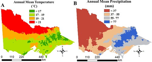
Temperature and rainfall data were collected from the Bureau of Meteorology of Australia for our study area between 2010 to 2020 (Figure 3A,B) (BOM 2021). The northwestern part of Victoria has the highest temperature and lowest precipitation while the northeastern part has the lowest temperature and highest precipitation (Figure 3A,B).

Figure 3. Climate conditioning factors for Victoria: (A) annual mean temperature, and (B) annual mean precipitation. The colour codes for each map are described in each figure.

2.2.2.3. Fuel loads

The NDVI and land cover data known as MODIS 1-km MYD13A3 NDVI (Figure 4A,B) were collected from USGS (USGS 2021). The majority of the eastern part of our study area has the highest NDVI index and is mainly covered by forests (Figure 4A,B). The western part is mainly covered by grassland, shrubland and savannas (Figure 4B) and these areas have the lowest NDVI index as well (Figure 4A).

Figure 4. Fuel load and human activity conditioning factors for Victoria: A) NDVI, (B) land cover, and (C) distance to roads. The colour codes for each map are described in each figure.

2.2.2.4. Human-made factors

Human activities are highly connected to the bushfires in the populated areas. Human activities, either voluntary (arsonism) or involuntary (accidental or negligent causes), can initiate fire (Leuenberger et al. 2018). In our research, distance to roads is considered as one of the human-made factors based on previous literature (Figure 4C). Open Street Map was used to calculate distance to roads (OSM 2021) which shows the variations in the study area. Another human-made factor to be considered is distance to populated areas, however, this factor is closely correlated with land cover which is already taken into account. Therefore, we excluded distance to populated areas. Distance to rivers is also excluded as this is correlated with land cover too.

2.3. Genetic programming

A Genetic Programming (GP) method is an extension of a genetic algorithm (GA) that was introduced by Koza (1992). The main difference between GP and GA is the representation of the solution (Gandomi et al. 2011; Mousavi et al. 2012). GP solutions are computer programs with hierarchical structures (Koza 1992; Gandomi et al. 2011; Mousavi et al. 2012), while GA solutions are strings of numbers (Mousavi et al. 2012). Hierarchical structures and the dynamic variability of computer programs are important features of GP (Koza 1992). GP starts with a random population of computer programs. Individuals are computer programs that have been measured based on their fitness and their performance in the special problem environment (Koza 1992). GP determines the fittest individuals that explain the problem (Koza 1992).

GP provides the outcome by running the following steps:

(1) Create an initial random population of computer programs which are a composite of functions and terminals.

(2) Execute following sub-steps repetitively and stop after a termination criterion has been met,

Perform each computer program in the population and allocate a fitness value to each program based on their ability to solve the problem.

Two main operations given below have to be used for the creation of new population. It is worthwhile to note that the fitness of computer programs will be considered for the following operations.

Computer programs will be copied to the next generation.

Two current genetic programs will be genetically recombined randomly to generate new computer programs.

(3) The best computer program resulted from any generation will be presented as the solution or an approximate solution to the problem (Koza 1992).

2.3.1. Gene expression programming

GEP was first introduced by Ferreira (2001) as an extension of GP. The nature of individuals is the main difference between GP and GEP. Individuals are nonlinear entities with different sizes and shapes representing as parse trees in GP, while individuals in GEP are linear strings with fixed lengths, but they will be expressed as nonlinear entities of different sizes and shapes (Ferreira 2001).

GEP starts with a random population of chromosomes. GEP works based on natural selection and the survival of the fittest. The best formula between inputs will be nominated by evolving the initial population through genetic operators (e.g. crossover and reproduction) (Hoang and Tien Bui 2018). We used GeneXproTools software to model the bushfire with GEP (Ferreira 2013).

GEP uses the following steps to nominate the best solution for the problem:

1. The first population of chromosomes will be generated randomly. Several genes will be linked by the linking function which will create chromosomes. Each chromosome has two parts that are called head and tail. Head can consist of functions and terminals while tail can be chosen only from terminals (Ferreira 2001; Hoang and Tien Bui 2018).

2. The fitness function will assign a value to each chromosome based on its performance (Hoang and Tien Bui 2018).

3. In the selection process, if the stop condition is not satisfied, the selection process will be applied based on the concept of roulette wheel with elitism. Hence each individual that is more fit has more chances to survive, and as a result, they are more likely to reproduce and the elitism replicates the best individuals to the next generation (Hoang and Tien Bui 2018).

4. The reproduction processes consist of several genetic operations including crossover, mutation, transposition, and inversion. These operations create diversity in the population. Crossover generates two new individuals through exchanging genetic elements between two random chromosomes. Two types of crossovers will be used in GEP (one-point and two-point crossovers). Mutation procedure randomly modifies the gene element at a certain point of a chromosome. Transposition is another genetic operation that can create diversity in the population by transporting gene fragments within the gene. Inversion operator can also randomly choose and then inverse the sequence in the chromosomes (Hoang and Tien Bui 2018).

2.4. Frequency ratio

Frequency ratio (FR) is a statistical method to generate the relationships between conditioning factors and independent variables (Hong et al. 2017; Razavi-Termeh et al. 2020). Bushfire prediction works based on the similarity of the conditions and characteristics of previous hazards (Razavi-Termeh et al. 2020). FR is a ratio of a bushfire area to the total study area which can be generated from Equation (1)(1) $$FR\left(x\right)=\frac{\frac{BF\left(x\right)}{\mathit{TBF}}}{\frac{N\left(x\right)}{TN}}$$(1) (Hong et al. 2017; Razavi-Termeh et al. 2020). (1) $$FR\left(x\right)=\frac{\frac{BF\left(x\right)}{\mathit{TBF}}}{\frac{N\left(x\right)}{TN}}$$(1) where BF(x) is the number of bushfires happened at a class x, TBF is the total number of bushfires, N(x) is the number of pixels in x, and TN is the total number of pixels for the whole study area. Each contributing factor to a bushfire can have multiple classes. For example, elevation can be reclassified as low, medium and high. For each factor f, FR(f) is the sum of the frequency ratios of the factor’s subclasses. And the bushfire susceptibility is the weighted sum of the factors’ frequency ratios. The weights should be determined by FR. Our weights are presented in Section 3. All factors and each factor’s subclasses used in our study are provided in Table 1. This FR method was reported to be an effective method for determining the importance and significance of different classes of factors (Van Westen et al. 2003; Hong et al. 2017).

Table 1. Frequency ratios for different subclasses of factors.

Factors	Subclass	Frequency ratio	Factors	Subclass	Frequency ratio
Elevation (m)	<172	0.466	Annual mean precipitation (mm)	<37	0.240
	172–379	1.100		37–55	0.370
	379–673	1.980		55–77	2.789
	673–1047	2.710		>77	2.230
	>1047	3.105	NDVI	<0.10	0.125
Aspect	North	0.755		0.10–0.29	0.107
	North east	0.870		0.29–0.44	0.440
	East	1.197		0.44–0.63	0.869
	South east	1.360		0.63–0.92	3.548
	South	1.068	Land cover	Forest	3.030
	South west	0.980		Shrublands	0.906
	West	0.973		Savannas	0.480
	North West	0.851		Grassland	0.249
	Flat	0.230		Wetland	0.200
Slope (degree)	0–1.1	0.353		Others	0.098
	1.1–3.2	1.942	Distance to roads (km)	<3	0.520
	3.2–6.0	2.765		3–8	1.224
	6.0–9.7	2.981		8–15	2.500
	>9.7	2.759		15–26	2.200
Annual mean temperature (°C)	<17	2.498		>26	0.495
	17–19	1.497
	19–21	0.750
	>21	0.200

2.5. Logistic regression

A Logistic Regression (LR) model can be used to determine the spatial relationship between bushfire occurrence and conditioning factors (Lee and Pradhan 2007). Correlations between the conditioning factors and bushfire occurrence have been calculated based on Equations (2)(2) $$\mathrm{p}=1/(1+e^{-z})$$(2) and (3)(3) $$\mathrm{z}=a_0+a_1{F}_1+a_2{F}_2+\dots +a_n{F}_n.$$(3) . (2) $$\mathrm{p}=1/(1+e^{-z})$$(2) where p is the probability of bushfire occurrence and z is a linear combination as follows: (3) $$\mathrm{z}=a_0+a_1{F}_1+a_2{F}_2+\dots +a_n{F}_n.$$(3) where a₀ is a model intercept, a₁, a₂, …, a_n are the coefficients of the model, and F_i’s are the independent conditioning factors (Lee and Pradhan 2007). The variables in LR can be either continuous or discrete due to the addition of a suitable link function to the ordinary linear regression (Lee and Pradhan 2007; Gholamnia et al. 2020). For this study, the dependent variable is binary. The R statistical software was used to carry out computational process (R Core team 2020).

2.6. An ensemble of GEP and FR (GEPFR)

The framework of an ensemble of GEP and FR (GEPFR) proposed in our research is illustrated in Figure 5. In the first step, eight factors and an inventory map were collected and classified. The importance of each class is assigned by FR. The data sets were randomly divided into training data (70%) and testing data (30%). The initial model is trained with 70% of the data (training data) based on the concept of GEP. The final model is evaluated by 30% of the data (testing data). Finally, a bushfire susceptibility map is generated by GEPFR.

Figure 5. The structure of an ensemble of GEP and FR (GEPFR) for bushfire susceptibility mapping.

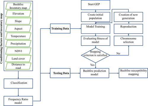
We used a population size of 30 where each chromosome has a head length of eight. Chromosomes in our study contain three genes that are linked together by applying addition. The terminal set consists of bushfire conditioning factors and constants. We chose functions (Table 2) based on the previous research (Ferreira 2013). We selected eight conditioning factors including elevation, aspect, slope, annual mean temperature, annual mean precipitation, NDVI, land cover, and distance to roads. The existing data were converted to raster layers. All conditioning factors except aspect and land cover were classified in ArcGIS using Natural break method. FR was used to evaluate the importance of different classes for each factor.

Table 2. Functions used in GEP.

Function	Symbol	Formula
Addition	+	X + Y
Subtraction	–	X–Y
Multiplication	*	X*Y
Division	/	X/Y
Logarithm	log	Log(X)
Average of two variables	avg	(X + Y)/2
Arctangent	Act	Arctan(X)
X to the power of two	X^2	X^2

The importance of conditioning factors was prioritized by GeneXproTools. For this purpose, the input variables were randomized, and their importance was defined based on the decreasing value of R-square between the generated model and real values (Ferreira 2013).

2.7. An ensemble of LR and FR (LRFR)

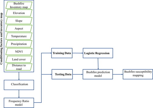
An ensemble of LR and FR (LRFR) is also used for bushfire susceptibility mapping. Factors were collected in the first step and then classified. The importance of each class is determined by FR, and then LR is trained by 70% of the data and is evaluated by 30% of the data (randomly chosen) (Figure 6). Finally, the bushfire susceptibility was generated.

Figure 6. The structure of an ensemble of LR and FR (LRFR) for bushfire susceptibility mapping.

3. Results and validation

The model was generated from GeneXproTools, and the resulting mathematical formula for bushfire susceptibility mapping by GEPFR is given in Equation (4)(4) $$\begin{array}{c}\mathrm{F}=\left(d_7+2\alpha \right)\times \left(\beta +d_1\right)\times \left(d_2\times d_6\right)+d_7\times \left(d_6+d_7-d_0\right)+{\left(\gamma -d_4\right)}^2\times {\left(d_5\times d_4\right)}^2+d_1-\delta \\ \mathrm{\alpha }=1.79,\mathrm{}\beta =5.44\mathrm{},\gamma =-4.06,\mathrm{}\delta =-0.88\end{array}$$(4) : (4) $$\begin{array}{c}\mathrm{F}=\left(d_7+2\alpha \right)\times \left(\beta +d_1\right)\times \left(d_2\times d_6\right)+d_7\times \left(d_6+d_7-d_0\right)+{\left(\gamma -d_4\right)}^2\times {\left(d_5\times d_4\right)}^2+d_1-\delta \\ \mathrm{\alpha }=1.79,\mathrm{}\beta =5.44\mathrm{},\gamma =-4.06,\mathrm{}\delta =-0.88\end{array}$$(4) where d₀ is aspect, d₁ is elevation, d₂ is land cover, d₃ is annual mean temperature, d₄ is NDVI, d₅ is annual mean precipitation, d₆ is distance to roads, and d₇ is slope. These are referred to as the weights mentioned in Subsection 2.4. α, β, γ, and δ are constant values that were determined by GEP.

Each sub-tree from Equation (4)(4) $$\begin{array}{c}\mathrm{F}=\left(d_7+2\alpha \right)\times \left(\beta +d_1\right)\times \left(d_2\times d_6\right)+d_7\times \left(d_6+d_7-d_0\right)+{\left(\gamma -d_4\right)}^2\times {\left(d_5\times d_4\right)}^2+d_1-\delta \\ \mathrm{\alpha }=1.79,\mathrm{}\beta =5.44\mathrm{},\gamma =-4.06,\mathrm{}\delta =-0.88\end{array}$$(4) is a gene that is linked together by the addition operator. The final result is the fittest chromosome. This chromosome contains three genus which consist of terminals and functions. A bushfire susceptibility map by GEPFR shows that the eastern part of Victoria is a hot spot for the bushfire occurrence, whereas the west seems to have the lowest possibility for the bushfire occurrence (Figure 7A). The AUCs of the model from the GEPFR in the training and testing sets are 0.863 and 0.860, respectively. Accuracy for training and testing sets are 91.12% and 90.79% respectively.

Figure 7. Bushfire susceptibility maps by (A) GEPFR, B) GEP, (C) LRFR, and (D) FR. The increasing probability of bushfire is represented on spectrum from dark green (very low) to red (very high).

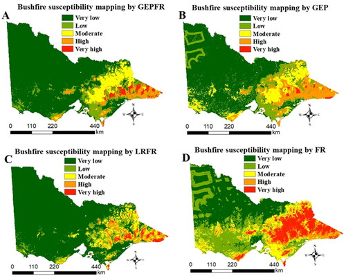
We also generated bushfires susceptibility maps by using a GEP method (Figure 7B). AUCs of the model generated by the GEP in the training and testing sets are 0.852 and 0.850, respectively. The training and testing sets have accuracies of 91.49% and 91.64%, respectively.

The LRFR generated a bushfire susceptibility map (Figure 7C) with the AUCs of 0.853 and 0.852 for training and testing sets, respectively. Accuracy is 92.4% for training and 92.2% for testing. The generated model from LRFR is given in Equation (5)(5) $$\mathrm{z}=-4.934+0.166\times As-0.339\times El+0.335\times L-0.232\times T+0.395\times N+0.528\times P+0.572\times D+0.200\times S$$(5) . (5) $$\mathrm{z}=-4.934+0.166\times As-0.339\times El+0.335\times L-0.232\times T+0.395\times N+0.528\times P+0.572\times D+0.200\times S$$(5) where, As is aspect, El is elevation, L is land cover, T is mean annual temperature, N is NDVI, P is mean annual precipitation, D is distance to roads and S is slope. These variables are referred to as the weights mentioned in Subsection 2.4.

Both training and testing sets have balanced AUCs and accuracies, which illustrates that there has been no overfitting in the presented models from all the used methods. It proves the generalization capabilities of the GEPFR, GEP, and LRFR methods for generation of bushfire models in Victoria.

We also generated bushfire susceptibility mapping by single FR (Figure 7D) which has AUC of 0.840 and accuracy of 81.2%. Our result shows that the GEPFR has the highest AUC compared to three other methods (GEP, LRFR, and FR). However, LRFR has the highest accuracy followed by GEP, GEPFR, and FR. Therefore, it is concluded that the two ensemble methods outperform the single methods. In summary, Table 3 shows the AUCs and accuracies of the four methods.

Table 3. Comparison parameters for different methods.

Methods	AUC	Accuracy
GEPFR	0.860	90.79%
GEP	0.850	91.64%
LRFR	0.852	92.27%
FR	0.840	81.23%

Bushfire susceptibility maps generated by the GEPFR, GEP, LRFR, and FR were reclassified by the natural break classification method. The reclassified maps were categorized into five subclasses including very low, low, moderate, high and very high (Figure 7A–D).

The natural break method uses patterns in data to generate break points that aims to minimize the variance within each class and maximize the variance between classes (Tehrany et al. 2019; Moayedi et al. 2020). Therefore, the susceptibility maps in our research were divided into five categories (Figure 7). The areas covered in each probability category are presented in Table 4 from different methods.

Table 4. Area covered in different bushfire susceptibility category from different methods.

Methods	Areas (%)
	Very low	Low	Moderate	High	Very High
GEPFR	71	12	8	6	3
GEP	59	15	13	12	1
LRFR	76	10	7	5	2
FR	33	31	13	10	13

The susceptibility maps in our research show that the majority of the eastern part of Victoria is prone to bushfire. The western part has the lowest bushfire susceptibility while it has the lowest annual mean precipitation and the highest annual mean temperature. East of Melbourne’s metropolitan area shows a moderate to high probability of bushfire. Also, the highest probability can be found in Croajingolong National Park located in eastern Victoria and Great Otway National Park located in South Victoria. These two areas have the highest NDVI. NDVI is low in the western part while it gradually increases toward the eastern part of Victoria. The majority of the area with a high bushfire probability in the eastern part is covered by forests and the western part with the lowest bushfire probability is covered by grasslands.

We divided the data into two sets including training and testing (randomly chosen, 70% and 30%, respectively) for GEPFR, GEP and LRFR. The best mathematical model as a solution for the problem was determined using the mentioned methods. The models were evaluated by Area Under Curve (AUC) of Receiver Operating Characteristic (ROC) and accuracy. Accuracy is a ratio of correctly classified cases to the number of all data (Hoang and Tien Bui 2018). ROC determines the efficiency of generated models. The AUC of ROC has been widely used in the assessment of the efficiency of predicted models (Bui 2019; Hong et al. 2019; Zhang et al. 2019; Pham et al. 2020; Razavi-Termeh et al. 2020; Eskandari et al. 2020a). Ling et al. (2003) proposed AUC of ROC for machine learning algorithms as an alternative single-number measure. The AUC is statistically consistent and more discriminating than accuracy (Ling et al. 2003). Hence, we use AUC to understand which method is presenting the best performance. The AUCs figure for different methods is also provided Figure 8. In the ROC curve, the false positive rate given in Equation (6)(6) $$\mathrm{FPR}=\frac{FP}{FP+TN}$$(6) is on X-axis, and the true positive rate in Equation (7)(7) $$\mathrm{TPR}=\frac{TP}{TP+FN}$$(7) is on Y-axis (Hong et al. 2019): (6) $$\mathrm{FPR}=\frac{FP}{FP+TN}$$(6) (7) $$\mathrm{TPR}=\frac{TP}{TP+FN}$$(7) where False Positive (FP) is the number of pixels that are wrongly classified as fire class, True Negative (TN) is the number of pixels that are correctly classified as non-fire class, True positive (TP) is the number of pixels that are correctly determined as fire class, and False Negative (FN) is the number of pixels that are wrongly classified as non-fire class (Hong et al. 2019). AUC values can be interpretated as < 0.6: poor, 0.6–0.7: moderate, 0.7–0.8: good, 0.8–0.9: very good and > 0.9: excellent classification (Hong et al. 2019). Accuracy in Equation (8)(8) $$\mathrm{Accuracy}\mathrm{}=\frac{TP+TN}{TP+TN+FP+FN}$$(8) is also one of the commonly used quality metrics for the comparison between different models. (8) $$\mathrm{Accuracy}\mathrm{}=\frac{TP+TN}{TP+TN+FP+FN}$$(8)

Figure 8. Map of ROCs for the tested methods.

4. Discussions

In this paper we introduced an innovative GEPFR for the prediction of bushfires in the Southeastern Australia. In our research, most of the bushfires were occurred in the eastern part of the Victoria because of high vegetation and fuel load in that area. GeneXproTools defines the importance of conditioning factors which indicate that NDVI plays an important role in bushfire occurrence in our study area. Similarly, previous research also reported that NDVI was an important factor in bushfires (Tien Bui et al. 2016; Zhang et al. 2016). The higher NDVI indicates the presence of more fuel load which is an important factor in the spread of fires (Zhang et al. 2016). Similarly, Tien Bui et al. (2017) stated that NDVI was the most important factor for bushfire occurrence and the highest probability of bushfire was found in the areas with high NDVI (Tien Bui et al. 2017). NDVI cannot distinguish different types of vegetation but can reflect variation in vegetation load, and as a result, it can be an important factor for bushfire prediction (Chen et al. 2001; Malak and Pausas 2006).

The eastern part of Victoria has the highest annual mean precipitation compared to the west and the annual mean precipitation is the second most important factor for our bushfire susceptibility mapping. Precipitation will increase vegetation and as a result, there will be a higher flammability rate in the area (Collins et al. 2014). Positive correlation between precipitation and bushfire occurrence in Southeastern Arizona also indicates that precipitation presumably increases the fuel load, however, climatic conditions cannot be extrapolated globally (Crimmins and Comrie 2004; Nicholls and Lucas 2007). In contrast, precipitation was the main negative driver for bushfire occurrence in Tasmania where lower precipitation led to the increase in the extent of burned areas (Nicholls and Lucas 2007).

In our study, temperature is higher in the western and northern part of Victoria, but these areas have low probabilities for bushfire. In contrast, some research reported that temperature is an important factor for bushfires in different areas (Hong et al. 2018; Gigović et al. 2019; Eskandari et al. 2020a). This contradictory result could be due to the land cover in the western and northern part of our study area. The western part is mainly covered by cropland, shrubland, and grassland which show lower association with bushfire occurrence. Similarly, previous research also shows that shrubland has the lowest probability for bushfire (Zhang et al. 2015, 2016). The western part has also the lowest annual precipitation rate and the highest temperature which results in a low amount of fuel load in the area.

Our models show that cropland, shrubland and grassland are less prone to bushfire and as a result there is lower bushfire possibility in the western part of Victoria which is covered by these types of plants. Grasslands have lower fuel load and mainly compaction in grasslands by weathering or grazing decreases the fire occurrence (Cheney 1976). Our research shows that most areas with a moderate to high probability of bushfire are covered by forests. Similarly, Zhang et al. (2016) reported that forest land cover had strong positive relationship with bushfires while shrubland had the lowest probability of bushfire.

In our study area, the bushfire occurrence was more frequent in the eastern area with higher elevation but our method shows that elevation is not among the most important factors. The elevation map correlates positively with forest vegetation which could explain the low importance of elevation factor for bushfire occurrence. Similarly, previous research showed that elevation corresponded with vegetation and as a result there was more bushfire in the elevated area because of higher vegetation (fuel load) (Zhang et al. 2016). Our results show that slope is not affecting bushfire occurrence. Similarly, slope was reported to have a weak relationship with the bushfire occurrence (Valdez et al. 2017; Eskandari et al. 2020a)

Comparison of bushfire susceptibility maps generated by GEPFR, GEP, LRFR, and FR show that the AUC of GEPFR is higher than the other three methods. LRFR also has a higher AUC than GEP. FR has the lowest AUC. The GEPFR, LRFR and GEP show that the majority of our study area has very low susceptibility for bushfires, while FR indicates that the majority of the area has very low to low susceptibility. The GEPFR is able to differentiate between very high and high prone areas, while GEP has nominated the majority of the eastern part as high category and FR has allocated 13% of the area as very high. GEPFR indicates that NDVI and precipitations are the most important factors. GEP determines that land cover, precipitation, and distance to roads are important. GEP also illustrates that forest had highest bushfire occurrence among different types of land cover. However, LRFR shows that distance to roads, precipitation, and NDVI play important roles in bushfire occurrence.

5. Concluding remarks

This research provides an insight to the use of GEPFR, GEP, LRFR, and FR to predict bushfires in Victoria, Australia. The inventory map of bushfires was generated using the historical bushfire data between 2010 and 2020. We used eight conditioning factors to prepare bushfire susceptibility maps for the case study area. The eastern part of Victoria has the highest probability of bushfire. This area is covered mostly with forest and has the highest NDVI. In summary, the bushfire susceptibility maps generated by the four proposed methods agree with the historical data in the area with low, moderate and high bushfire probabilities.

Data and codes availability statement

The data is available in: https://github.com/maryam929/MH_Data.git

Disclosure statement

There are no relevant financial or non-financial competing interests.

References

- BOM. 2021. Australia’s Official Weather Forecasts and Weather Radar - Bureau of Meteorology. [accessed 2020 Dec 01]. http://www.bom.gov.au/.
- Bui QT. 2019. Metaheuristic algorithms in optimizing neural network: a comparative study for forest fire susceptibility mapping in Dak Nong, Vietnam. Geomat Nat Hazards Risk. 10 (1):136–150.
- Bunch A. 2020. Australia bushfire latest: state-by-state breakdown of all areas affected by blazes. [accessed 2021 Jan 01]. https://7news.com.au/news/bushfires/australia-bushfire-latest-state-by-state-breakdown-of-all-areas-affected-by-blazes-c-630858.
- Catry FX, Rego FC, Bação FL, Moreira F. 2009. Modeling and mapping wildfire ignition risk in Portugal. Int J Wildland Fire. 18(8):921–931.
- Chen K, Jacobson C, Blong R. 2001. Using NDVI image texture analysis for bushfire-prone landscape assessment. Asian Conf Remote Sens. 22(9):1–9.
- Cheney NP. 1976. Bushfire disasters in Australia, 1945-1975. Aust For. 39(4):245–268.
- Clarke H, Gibson R, Cirulis B, Bradstock RA, Penman TD. 2019. Developing and testing models of the drivers of anthropogenic and lightning-caused wildfire ignitions in south-eastern Australia. J Environ Manage. 235:34–41.
- Collins L, Bradstock RA, Penman TD. 2014. Can precipitation influence landscape controls on wildfire severity’ A case study within temperate eucalypt forests of south-eastern Australia. Int J Wildland Fire. 23(1):9–20.
- Crimmins MA, Comrie AC. 2004. Interactions between antecedent climate and wildfire variability across south-eastern Arizona. Int J Wildland Fire. 13(4):455–466.
- De Vasconcelos MJP, Silva S, Tome M, Alvim M, Pereira JMC. 2001. Spatial prediction of fire ignition probabilities: comparing logistic regression and neural networks. Photogramm Eng Remote Sensing. 67(1):73–81.
- Dorji S, Ongsomwang S. 2017. Wildfire susceptibility mapping in Bhutan using geoinformatics technology. Suranaree J Sci Technol. 24(2):213–237.
- Emamgolizadeh S, Bateni SM, Shahsavani D, Ashrafi T, Ghorbani H. 2015. Estimation of soil cation exchange capacity using Genetic Expression Programming (GEP) and Multivariate Adaptive Regression Splines (MARS). J Hydrol. 529:1590–1600. https://doi.org/http://dx.doi.org/10.1016/j.jhydrol.2015.08.025.
- Eskandari S, Amiri M, Sãdhasivam N, Pourghasemi HR. 2020a. Comparison of new individual and hybrid machine learning algorithms for modeling and mapping fire hazard: a supplementary analysis of fire hazard in different counties of Golestan Province in Iran. Nat Hazards. 104(1):305–327.
- Eskandari S, Miesel JR, Pourghasemi HR. 2020b. The temporal and spatial relationships between climatic parameters and fire occurrence in northeastern Iran. Ecol Indic. 118:106720.
- Ferreira C. 2001. Gene expression programming: a new adaptive algorithm for solving problems. [accessed 2021 Mar 8]. https://arxiv.org/abs/cs/0102027
- Ferreira C. 2013. Gepsoft GeneXproTools - Data modeling & analysis software. [accessed 2021 Mar 8]. https://www.gepsoft.com/.
- Gandomi AH, Tabatabaei SM, Moradian MH, Radfar A, Alavi AH. 2011. A new prediction model for the load capacity of castellated steel beams. J Constr Steel Res. 67(7):1096–1105. https://doi.org/http://dx.doi.org/10.1016/j.jcsr.2011.01.014.
- Gholamnia K, Gudiyangada Nachappa T, Ghorbanzadeh O, Blaschke T. 2020. Comparisons of diverse machine learning approaches for wildfire susceptibility mapping. Symmetry. 12(4):604.
- Ghorbanzadeh O, Blaschke T, Gholamnia K, Aryal J. 2019a. Forest fire susceptibility and risk mapping using social/infrastructural vulnerability and environmental variables. Fire. 2(3):27–50.
- Ghorbanzadeh O, Feizizadeh B, Blaschke T. 2018. Multi-criteria risk evaluation by integrating an analytical network process approach into GIS-based sensitivity and uncertainty analyses. Geomat Nat Hazards Risk. 9(1):127–151.
- Ghorbanzadeh O, Kamran KV, Blaschke T, Aryal J, Naboureh A, Einali J, Bian J. 2019b. Spatial prediction of wildfire susceptibility using field survey GPS data and machine learning approaches. Fire. 2(3):23–43.
- Gigović L, Pourghasemi HR, Drobnjak S, Bai S. 2019. Testing a new ensemble model based on SVM and random forest in forest fire susceptibility assessment and its mapping in Serbia’s Tara National Park. Forests. 10(5):408.
- Gralewicz NJ, Nelson TA, Wulder MA. 2012. Factors influencing national scale wildfire susceptibility in Canada. For Ecol Manage. 265:20–29. https://doi.org/http://dx.doi.org/10.1016/j.foreco.2011.10.031.
- Green ME, Deluca TF, Kaiser KWD. 2020. Modeling wildfire using evolutionary cellular automata. GECCO 2020 – Proceedings of the 2020 Genetic and Evolutionary Computation Conference; Cancún, Mexico. p. 1089–1097. https://doi.org/https://doi.org/10.1145/3377930.3389836
- Hoang ND, Tien Bui D. 2018. Spatial prediction of rainfall-induced shallow landslides using gene expression programming integrated with GIS: a case study in Vietnam. Nat Hazards. 92(3):1871–1887.
- Hong H, Jaafari A, Zenner EK. 2019. Predicting spatial patterns of wildfire susceptibility in the Huichang County, China: an integrated model to analysis of landscape indicators. Ecol Indic. 101:878–891.
- Hong H, Naghibi SA, Moradi Dashtpagerdi M, Pourghasemi HR, Chen W. 2017. A comparative assessment between linear and quadratic discriminant analyses (LDA-QDA) with frequency ratio and weights-of-evidence models for forest fire susceptibility mapping in China. Arab J Geosci. 10(7): 167.
- Hong H, Tsangaratos P, Ilia I, Liu J, Zhu AX, Xu C. 2018. Applying genetic algorithms to set the optimal combination of forest fire related variables and model forest fire susceptibility based on data mining models. The case of Dayu County, China. Sci Total Environ. 630:1044–1056.
- Jaafari A, Gholami DM, Zenner EK. 2017. A Bayesian modeling of wildfire probability in the Zagros Mountains, Iran. Ecol Inform. 39:32–44.
- Jaafari A, Mafi-Gholami D, Thai Pham B, Tien Bui D. 2019c. Wildfire probability mapping: Bivariate vs. Multivariate statistics. Remote Sens. 11(6):618.
- Jaafari A, Pourghasemi HR. 2019. Factors influencing regional-scale wildfire probability in Iran. In: In Spatial modeling in GIS and R for Earth and environmental sciences. Elsevier; p. 607–619. https://doi.org/https://doi.org/10.1016/b978-0-12-815226-3.00028-4.
- Jaafari A, Razavi Termeh SV, Bui DT. 2019a. Genetic and firefly metaheuristic algorithms for an optimized neuro-fuzzy prediction modeling of wildfire probability. J Environ Manage. 243:358–369.
- Jaafari A, Zenner EK, Panahi M, Shahabi H. 2019b. Hybrid artificial intelligence models based on a neuro-fuzzy system and metaheuristic optimization algorithms for spatial prediction of wildfire probability. Agric for Meteorol. 266–267:198–207.
- Jaafari A, Zenner EK, Pham BT. 2018. Wildfire spatial pattern analysis in the Zagros Mountains, Iran: a comparative study of decision tree based classifiers. Ecol Inform. 43:200–211.
- Jain P, Coogan SCP, Subramanian SG, Crowley M, Taylor S, Flannigan MD. 2020. A review of machine learning applications in wildfire science and management. Environ. Rev.28(4): 478-505.https://doi.org/https://doi.org/10.1139/er-2020-0019
- Kayadelen C. 2011. Soil liquefaction modeling by genetic expression programming and neuro-fuzzy. Expert Syst Appl. 38(4):4080–4087.
- Koza JR. 1992. Genetic programming : On the programming of computers by means of natural selection complex adaptive systems. (Vol. 1). MIT press.
- Lee S, Pradhan B. 2007. Landslide hazard mapping at Selangor, Malaysia using frequency ratio and logistic regression models. Landslides. 4(1):33–41.
- Leonard J, Blanchi R. 2012. Queensland Bushfire Risk Planning Project. Stage 1 Report for the Department of Community Safety–Strategic Policy Division Final Version–Approved by CSIRO, July.
- Leuenberger M, Parente J, Tonini M, Pereira MG, Kanevski M. 2018. Wildfire susceptibility mapping: deterministic vs. stochastic approaches. Environ Model Softw. 101:194–203.
- Ling CX, Huang J, Zhang H. 2003. AUC: a statistically consistent and more discriminating measure than accuracy. IJCAI Int Jt Conf Artif Intell. 3: 519–524.
- Malak DA, Pausas JG. 2006. Fire regime and post-fire Normalized Difference Vegetation Index changes in the eastern Iberian Peninsula (Mediterranean basin). Int J Wildland Fire. 15(3):407–413.
- Moayedi H, Mehrabi M, Bui DT, Pradhan B, Foong LK. 2020. Fuzzy-metaheuristic ensembles for spatial assessment of forest fire susceptibility. J Environ Manage. 260:109867.
- Mousavi SM, Aminian P, Gandomi AH, Alavi AH, Bolandi H. 2012. A new predictive model for compressive strength of HPC using gene expression programming. Adv Eng Softw. 45(1):105–114. https://doi.org/http://dx.doi.org/10.1016/j.advengsoft.2011.09.014.
- Nicholls N, Lucas C. 2007. Interannual variations of area burnt in Tasmanian bushfires: relationships with climate and predictability. Int J Wildland Fire. 16(5):540–546.
- O’Connor CD, Thompson MP, Rodríguez y Silva F. 2016. Getting ahead of the wildfire problem: quantifying and mapping management challenges and opportunities. Geosciences. 6(3):35.
- OSM. 2021. OpenStreetMap. [accessed 2020 Dec 01]. https://www.openstreetmap.org/#map=4/-28.15/133.28.
- Pham BT, Jaafari A, Avand M, Al-Ansari N, Du T,H, Yen HP, Phong T, Van Nguyen DH, Van Le H, Mafi-Gholami D, et al. 2020. Performance evaluation of machine learning methods for forest fire modeling and prediction. Symmetry (Basel). 12(6):1022.
- Pourghasemi HR. 2016. GIS-based forest fire susceptibility mapping in Iran: a comparison between evidential belief function and binary logistic regression models. Scand J for Res. 31(1):80–98.
- R Core Team. 2020. R: a language and environment for statistical computing. Vienna (Austria): R Foundation for Statistical Computing. [accessed 2021 Dec 05]. https://www.R-project.org/.
- Razavi-Termeh SV, Sadeghi-Niaraki A, Choi SM. 2020. Ubiquitous GIS-based forest fire susceptibility mapping using artificial intelligence methods. Remote Sens. 12(10):1689.
- Sachdeva S, Bhatia T, Verma AK. 2018. GIS-based evolutionary optimized Gradient Boosted Decision Trees for forest fire susceptibility mapping. Nat Hazards. 92(3):1399–1418.
- Shang C, Wulder MA, Coops NC, White JC, Hermosilla T. 2020. Spatially-explicit prediction of wildfire burn probability using remotely-sensed and ancillary data. Can J Remote Sens. 46(3):1–17.
- Tehrany MS, Jones S, Shabani F, Martínez-Álvarez F, Tien Bui D. 2019. A novel ensemble modeling approach for the spatial prediction of tropical forest fire susceptibility using LogitBoost machine learning classifier and multi-source geospatial data. Theor Appl Climatol. 137(1–2):637–653.
- Tien Bui D, Bui QT, Nguyen QP, Pradhan B, Nampak H, Trinh PT. 2017. A hybrid artificial intelligence approach using GIS-based neural-fuzzy inference system and particle swarm optimization for forest fire susceptibility modeling at a tropical area. Agric For Meteorol. 233:32–44. https://doi.org/http://dx.doi.org/10.1016/j.agrformet.2016.11.002.
- Tien Bui D, Le KTT, Nguyen VC, Le HD, Revhaug I. 2016. Tropical forest fire susceptibility mapping at the Cat Ba National Park area, Hai Phong City, Vietnam, using GIS-based Kernel logistic regression. Remote Sens. 8(4):315–347.
- Tolhurst KG, Shields B, Chong DM. 2008. Phoenix: development and application of a bushfire risk management tool. Aust J Emerg Manag. 23(4):47.
- Tonini M, D’andrea M, Biondi G, Esposti SD, Trucchia A, Fiorucci P. 2020. A machine learning-based approach for wildfire susceptibility mapping. The case study of the Liguria region in Italy. Geosciences. 10(3): 105.
- USGS. 2021. EarthExplorer. [accessed 2020 Dec 01]. https://earthexplorer.usgs.gov.
- Valdez MC, Chang KT, Chen CF, Chiang SH, Santos JL. 2017. Modelling the spatial variability of wildfire susceptibility in Honduras using remote sensing and geographical information systems. Geomat Nat Hazards Risk. 8(2):876–892.
- Van Westen CJ, Rengers N, Soeters R. 2003. Use of geomorphological expert knowledge in indirect landslide hazard assessment. Nat Hazards. 30(3):399–419.
- Werner J, Lyons S. 2020. The size of Australia’s bushfire crisis captured in five big numbers. ABC Sci. [accessed 2021 Mar 8]. https://www.abc.net.au/news/science/2020-03-05/bushfire-crisis-five-big-numbers/12007716.
- You W, Lin L, Wu L, Ji Z, Yu J, Zhu J, Fan Y, He D. 2017. Geographical information system-based forest fire risk assessment integrating national forest inventory data and analysis of its spatiotemporal variability. Ecol Indic. 77:176–184. https://doi.org/http://dx.doi.org/10.1016/j.ecolind.2017.01.042.
- Zakaria NA, Azamathulla HM, Chang CK, Ghani AA. 2010. Gene expression programming for total bed material load estimation-a case study. Sci Total Environ. 408(21):5078–5085. https://doi.org/http://dx.doi.org/10.1016/j.scitotenv.2010.07.048.
- Zhang G, Wang M, Liu K. 2019. Forest fire susceptibility modeling using a convolutional neural network for Yunnan Province of China. Int J Disaster Risk Sci. 10(3):386–403.
- Zhang Y, Lim S, Sharples JJ. 2015. Development of spatial models for bushfire occurrence in South-Eastern Australia. 21st International Congress on Modelling and Simulation, Gold Coast, Australia. https://116.90.59.164/modsim2015/A4/zhang.pdf.
- Zhang Y, Lim S, Sharples JJ. 2016. Modelling spatial patterns of wildfire occurrence in South-Eastern Australia. Geomat Nat Hazards Risk. 7(6):1800–1815.