A hybrid recognition model of microseismic signals for underground mining based on CNN and LSTM networks

Abstract

Microseismic (MS) monitoring technology has been widely used to monitor ground pressure disasters. However, the underground mining environment is complex and contains many types of noise sources. Furthermore, the traditional recognition method entails a complex process with low recognition accuracy for MS signals, so it is difficult to serve for the safe production of mines. Therefore, this study established a hybrid model combining the singular spectrum analysis (SSA) method, convolutional neural networks (CNN), and long short-term memory networks (LSTM). First, the principal components of monitoring signals were extracted with the SSA method, and then spatial and temporal features of monitoring signals were separately extracted with the CNN and LSTM. Based on actual field data collected from Xiadian Gold Mine, the hybrid model was compared with the CNN, LSTM, and back-propagation networks (BP), as well as commonly used recognition methods including the support vector machine (SVM), decision tree (DT), K-nearest neighbor (KNN), and linear discriminant analysis (LDA). The results show that the proposed hybrid model can accurately extract data features of monitoring signals and further improve MS signals' recognition performance. Furthermore, the recognition accuracy of mechanical signals in monitoring signals is particularly increased using the hybrid model, which avoids confusion with MS signals.

Keywords:

• Mine microseismic monitoring
• convolutional neural networks
• long short-term memory
• signal recognition

1. Introduction

The deformation and failure of rock masses essentially mean the initiation, propagation, and interaction of fractures under engineering-induced disturbance, during which microseismic (MS) signals are released and can be synchronously recorded by multiple MS sensors distributed in the vicinity (Dai et al. 2017; Zhao et al. 2019). Performing inversion analysis on the MS signals containing rock failure information can rapidly acquire important data such as three factors (i.e., time, location, and magnitude) pertinent to rock failure and source mechanisms (Backers et al. 2005). However, sensors for MS monitoring are arranged in a harsh environment. Under challenging circumstances in mines where many mining activities are co-occurring, the collected signals are diverse. The signals that are not caused by rock mass failure akin to MS signals can be captured by the MS monitoring system, which will reduce the accuracy of interpretation of mine disasters (Zhao et al. 2020). Therefore, the application effects of MS monitoring in mines largely depend on how accurately MS signals are recognized.

For commonly used MS monitoring systems, the frequency and amplitude of signals can be set to pre-process the triggered signals. Despite this, due to the complex underground environment, the parameters of noise signals change significantly, and the ranges of frequency and amplitude are broad, so it is challenging to remove signals other than MS signals through a threshold given by the system. In addition, some valid MS signals will be filtered out because of poor parameter settings. The recognition performance of MS signals is significant to determine source location, calculate source parameters, and infer likely source mechanisms (Xue et al. 2016). The above-mentioned scientific problems have always been the research focus of scholars.

At present, studies on recognition of MS monitoring signals in underground mines mainly focus on the recognition of MS and blasting signals using time-frequency analysis (Arrowsmith et al. 2006; Allmann et al. 2008; Quang et al. 2015), recognition methods with combined multiple parameters (Dong et al. 2014, 2016a; Ma et al. 2015; Li et al. 2018), and machine learning method (Vallejos and McKinnon 2013; Li et al. 2015). For example, Allmann et al. (2008) obtained the magnitude-frequency characteristics of MS signals through Fourier transformation, which provides a basis for preliminarily identifying MS and blasting signals of rock masses. According to the non-linear characteristics of monitoring signal, Dong et al. (2016a) selected the occurrence time, seismic moment, total radiant energy, the ratio of S-wave to P-wave amplitude, corner frequency, and static stress drop of MS events as characteristic parameters to recognize MS signals. Vallejos and Mckinnon (2013) selected 13 characteristic parameters of MS signals as input indices of logistic regression and neural network pattern recognition and discussed their advantages and disadvantages. Although these parameters and algorithms show a certain degree of accuracy, there are still some shortcomings. The time-frequency analysis method can only preliminarily recognize MS signals and has the local contradiction between time domain and frequency domain and poor adaptive decomposability. The multi-parameter analysis method can recognize MS signals, but its characteristic parameters are complex, and there are some common parts among source parameters, so its implementation is complex.

Furthermore, Li et al. (2015) recognized MS signals through empirical mode decomposition (EMD), which enhances the characteristics of MS signals. However, it is challenging to analyze large-scale training samples and solve multi-recognition problems using the traditional machine learning method (Pu et al. 2019), such as Back-Propagation neural network (BP), EMD, and SVM. There often face over-envelope, under-envelope, modal mixing, and noticeable end effects. Furthermore, the traditional machine learning method lacks the ability of learning, fault tolerance, and fuzzy identification based on prior knowledge, and the self-adaptive ability of the identification model is poor. Therefore, it can only be applied to identifying MS signals under specific conditions with a low degree of intelligence.

The above methods of MS signal recognition need to manually extract features from the original data based on signal processing and statistical theories. The disadvantage is that it needs a lot of engineering practice and information processing technology to extract signal features, which seriously depends on the professional knowledge of personnel (Zhang et al. 2020). Furthermore, signals captured by the MS monitoring system in mines include MS and blasting signals and some mechanical signals with low frequency and amplitude (which are easily confused with MS signals). Therefore, the recognition of MS signals is a multi-recognition problem. Due to the complexity of the mine environment and the scattering and reflection effect of the rock, the energy, and frequency of monitoring signals are constantly decreasing, which is characterized by diversity and complexity (Xu et al. 2010). Therefore, the monitored signals are so massive that the traditional feature extraction and signal recognition methods are rendered inapplicable for the MS monitoring system used in the mine, which leads to the accurate identification of MS signals become a challenging topic.

Although many scholars combined data statistics technology, signal processing technology, and neural networks technology to realize the preliminary identification of MS signals on the computer, the final identification result is still based on the later artificial intervention. In the early stage of the automatic recognition model, the feature parameters need to be provided manually. Furthermore, the recognition criterion is single, which significantly affects the accuracy and reliability of recognition, and has no deep learning ability. In recent years, deep learning technology provides an effective tool to solve the above problems.

At present, due to the excellent feature extraction ability of deep learning technology than traditional methods, it has achieved great success in computer vision, machine translation, signal processing, and other fields (Lv et al. 2019; Singh et al. 2021). However, the research in mine MS monitoring is still in its infancy (Dong et al. 2020). At present, the feature learning ability of the convolutional neural network (CNN) has been recognized and rapidly developed with the advances made possible by modern computers and big-data techniques (Gu et al. 2018). It has made breakthrough achievements in image recognition (Alex et al. 2012), speech recognition (Abdel-Hamid et al. 2014), and heartbeat and brain waves fields (Kiranyaz et al. 2016) while remaining rare in applications to MS monitoring in mines. However, the information in the CNN is transferred unidirectionally, and there is no connection between the nodes in each layer, so it is impossible to simulate time-dependent relationships therewith. Furthermore, due to the complexity of MS monitoring signals, the features of the original time series of signals are generally ignored when extracting monitoring signals only using CNN. As a result, the CNN can only extract the local spatial features of the monitoring signal but not the time-domain features.

A recurrent neural networks (RNN) model- long short-term memory networks (LSTM) has a cyclic network structure and the ability to memorize historical information. That is to say; the LSTM can extract the time domain characteristics of time-series signals. At present, the LSTM has been widely used for the analysis of time-series signals, such as those required for traffic speed prediction (Ma et al. 2015), power load forecasting (Jian et al. 2017; Kong et al. 2019) and speech recognition (Graves and Jaitly 2014). However, in the mine MS monitoring field, scholars have done little research on the LSTM in MS signal recognition. As a result, they have not effectively combined the advantage of LSTM with the time-series feature of the MS signal. However, the disadvantage of the LSTM is that they can only extract the temporal features of signals but not the local spatial features.

Given the spatial and temporal features of monitoring signals, it is hard to extract the two types of features in a single network structure simultaneously. Hence, a new hybrid networks model (SSA-CNN-LSTM) for identifying all kinds of monitoring signals generated during mining based on singular spectrum analysis (SSA) (for extracting valid signal components), CNN (for extracting spatial feature), and LSTM (for extracting temporal feature) is proposed. Considering that the monitoring signal is usually the superposition of multiple signals, the principal component of the monitoring signal is extracted by SSA before extracting the spatio-temporal features of the monitoring signal, thus enhancing the distinction between different types of monitoring signals. Then, combining the advantages of CNN and LSTM, the former is used to extract the local spatial characteristics of the signal, and the latter is used to extract the temporal characteristics of the signal. Based on the experimental data of MS monitoring signals recorded in a test stope in the Xiadian Gold Mine (Shandong Province, China), the accuracy of the SSA-CNN-LSTM at recognizing signals was verified. The study aims to improve the recognition performance of MS signals, providing a new idea to recognize and study MS monitoring signals in the mine.

2. Engineering background and data source

2.1. Engineering background

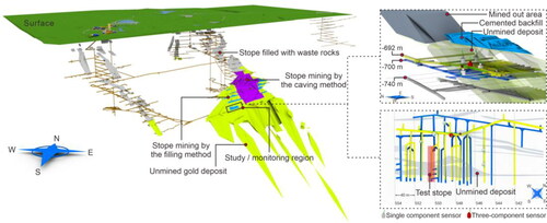
The Xiadian Gold Mine located in Zhaoyuan City, the ‘gold capital’ of China, is one of ten mines producing gold in China. The vein-like and quasi-lamellar main orebody of the mine occurs at elevations in the range of –600 to –1470 m and undulates gently and wavily along with the strike and dip (left panel, Figure 1). The Xiadian Gold Mine, with a current mining depth of 800 m, typifies deep mining operations in China. The underground mining environment in the mining area is adverse, especially under the long-term effect of high in situ stress. Much elastic energy accumulates in the surrounding rocks, which poses a risk of severe ground pressure behavior. At present, to achieve the economic and safety goals of efficient mining, a test stope (lower right panel, Figure 1) was set at a sub-level of –700 m in the mine to perform optimization testing of the stope structure. In addition, the IMS MS monitoring system commonly used in mines was distributed near the test stope to monitor the stability of the test stope. Based on the prevailing conditions on-site, six MS sensors (five single-component geophones and one three-component geophone with bandwidth of 9 to 2000 Hz and sensitivity of 80 V/m/s ± 10%) with 6000 Hz sampling frequency were distributed near the sub-levels of –692 m and –700 m in the test stope, guaranteeing favorable location accuracy of MS events. Four and two MS sensors were separately distributed at sub-levels of –692 m and –700 m, respectively, as shown in the right panel in Figure 1. MS sensors were densely arranged in the range of 4109,813.06 m to 4109,931.55 m in the north and 529,676.57 m to 529,753.62 m in the East.

Figure 1. Three-dimensional model of the Xiadian Gold Mine.

2.2. Data source and its characteristics

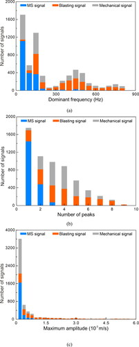
According to the blasting time and place recorded on-site, the blasting signals are manually selected as templates to identify all monitored signals to determine the blasting signal manually. Next, judge the signals obtained when the mine has no blasting, and there are few mechanical signals, and manually screen out the MS signals. These signals are used as references to identify all monitored signals to determine the MS signal manually. Finally, the signals monitored during the operation of mechanical equipment are analyzed and based on this, manual recognition of all monitored signals is made to determine mechanical signals. As a result, 7164 signals were collected from the MS monitoring system (from December 11, 2015, to February 29, 2016) before, during, and after mining in Xiadian Gold Mine, including 2765 MS signals, 2381 blasting signals, and 2018 mechanical signals. It is pointed out in (Hensman and Masko 2015) that the balanced distribution yielded the best performance. Therefore, a signal database containing three types of signals is established manually by carefully analyzing the monitoring signal. This signal database contains 2000 MS signals, 2000 blasting signals, and 2000 mechanical signals. The three common types of signals recorded in the MS monitoring system are shown in Figure 2. Figure 3 shows the statistical results of dominant frequencies, number of peaks, and maximum amplitude of the three common types of signals.

Figure 2. Three common types of signals recorded in MS monitoring system: (a) MS signal, (b) blasting signal, and (c) mechanical signal.

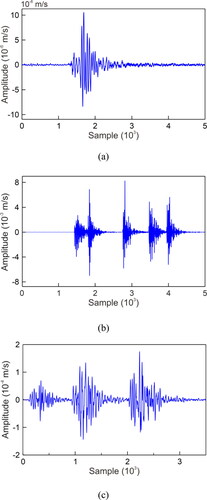
Figure 3. Histogram of characteristic parameters of three kinds of signals: (a) dominant frequency, (b) number of peaks and (c) maximum amplitude.

As shown in Figures 2 and 3:

1. A typical MS signal is illustrated in Figure 2(a). This kind of signal is released by rock failure, showing slow signal attenuation and developed coda. The amplitude is lower than that of blasting signals and mechanical signals, and the dominant frequency is low, generally below 200 Hz. In addition, this kind of MS signal usually contains one peak.

2. A typical blasting signal is shown in Figure 2(b). Since metal mines are mostly excavated and mined through blasting, many blasting signals are recorded in monitoring signals, with higher amplitude and wider dominant frequency range than MS signals. In addition, they have the characteristics of high amplitude, fast attenuation, and multiple peaks.

3. A typical mechanical signal is shown in Figure 2(c). There are many mechanical equipment operations during mining in the underground mine, such as fans and drilling rigs, mine car transportation, truck transportation, and ore-drawing. Such signals have a long duration, slower attenuation, and wider dominant frequency range than MS signals. However, its developed coda is similar to MS signals. Moreover, because underground mechanical equipment produces many mechanical signals, and their signals are complex and diverse, it is difficult to distinguish them from MS signals.

There are many similarities among the above three types of signals (Figure 3), so it is challenging to recognize MS signals directly from amplitude or dominant frequency alone. In addition, due to the complex transmission paths of MS signals, phenomena such as reflection, diffraction, and attenuation will occur in the transmission of signals in geologic media. Moreover, signals also interfere with each other, which determines the complexity of signals and increases the difficulty of signal identification.

3. A new signal recognition model—SSA-CNN-LSTM

In this section, with the help of the SSA method, CNN, and LSTM, a new hybrid signal recognition model (SSA-CNN-LSTM) is proposed, which is the core content of this article. The basis of selecting the SSA method is that this method can extract valid components of monitoring signals and weaken background noise, thus improving the discrimination of the signals (Zhigljavsky 2010). The monitoring signal processed by the SSA method forms an RGB image through the short-time Fourier transform (STFT) method, which is used as the input of the proposed hybrid model. The basis of selecting CNN is that CNN has a strong learning ability for image features, which can extract spatial features of monitoring signals. The basis of selecting the LSTM is that LSTM can memorize the historical information and thus shows the unique superiority in processing the sequence signals.

3.1. SSA method

Using the SSA method, the data space is projected into sub-spaces with different features, and singular values characterize the nature of these sub-spaces. This method realizes the function of extracting principal components of signals based on the reduced-rank principle (Vautard and Ghil 1989) and can recognize different frequencies of signals and rank the signals by signal energy. It mainly includes three parts: calculation of trajectory matrix, singular value decomposition of the matrix, and reconstruction of principal components of signals.

The deduction behind the method is described as follows (Vautard and Ghil 1989; Groth and Ghil 2015):

A one-dimensional time-series monitoring signal is assumed to be $\mathit{x}=[x_1,x_2,\dots ,x_N].$ To understand its implicit construct of temporal evolution, the monitoring signals are arranged with a time lag. (1) $$\mathbf{X}=\left[\begin{array}{cccc}{x}_1& x_2& \cdots & x_{N-M+1}\\ x_2& x_3& \cdots & x_{N-M+2}\\ ⋮& ⋮& \ddots & ⋮\\ x_M& x_{M+1}& \cdots & x_N\end{array}\right]$$(1) where, time lag M refers to window length or embedding dimension. The embedding dimension M is equivalent to the resolution when decomposing components of monitoring signals. The above matrix X is named the trajectory matrix. The trajectory matrix is a Hankel matrix, and all elements on the anti-diagonal are equal. Its autocovariance matrix is expressed as follows: (2) $${\mathbf{T}}_X=\left[\begin{array}{cccc}c(0)& c(1)& \cdots & c(M-1)\\ c(1)& c(0)& \cdots & c(M-2)\\ ⋮& ⋮& \ddots & ⋮\\ c(M-1)& c(M-2)& \cdots & c(0)\end{array}\right]$$(2) where, ${\mathbf{T}}_X$ represents a Toeplitz matrix, in which elements on the main diagonal are equal, as are the elements on the line parallel to the main diagonal. It is widely applied in digital signal processing.

The reason for constructing the covariance matrix is that it can judge the correlation of data. The larger the singular value of the covariance matrix, the closer the original series is distributed to the eigenvector corresponding to the singular value. Therefore, the waveform reconstructed by the eigenvector can represent the main features of the original series. $c(j)$ denotes the serial estimation of time series signal x, which can be calculated by Yule-Walke estimation. (3) $$c(j)=\frac{1}{N-j}\sum _{t=1}^{N-j}{x}_t{x}_{t+j},(j=0,1,2,\dots ,M-1)$$(3)

By performing singular value decomposition on ${\mathbf{T}}_X,$ the singular value vector $\mathbf{\lambda }$ and the corresponding eigenvector matrix E can be obtained, expressed as follows: (4) $$\mathbf{\lambda }=[{\lambda }_1,{\lambda }_2,\dots ,{\lambda }_M]$$(4) (5) $$\mathbf{E}=[{\mathbf{E}}_1,{\mathbf{E}}_2,\dots ,{\mathbf{E}}_M]=\left[\begin{array}{cccc}{E}_{1,1}& E_{1,2}& \cdots & E_{1,M}\\ E_{2,1}& E_{2,2}& \cdots & E_{2,M}\\ ⋮& ⋮& \ddots & ⋮\\ E_{M,1}& E_{M,2}& \cdots & E_{M,M}\end{array}\right]$$(5) where, the singular value meets $\left|{\lambda }_1\right|\ge \left|{\lambda }_2\right|\ge \cdots \ge \left[{\lambda }_M\right];$ ${\mathbf{E}}_1,$${\mathbf{E}}_2,$…,${\mathbf{E}}_M$ denote m eigenvectors in ${\mathbf{T}}_X.$

The singular value vector $\mathbf{\sigma }$ of ${\mathbf{T}}_X$ is given by: (6) $$\mathbf{\sigma }=\left[{\sigma }_1,{\sigma }_2,\dots ,{\sigma }_M\right]=\left[\sqrt{\left|{\lambda }_1\right|},\sqrt{\left|{\lambda }_2\right|},\dots ,\sqrt{\left|{\lambda }_M\right|}\right]$$(6) where, $\mathbf{\sigma }$ is called the singular spectrum of MS signal x, and singular spectrum analysis is to calculate its singular value. The eigenvector corresponding to ${\lambda }_k$ is the k^th-order mode, and each mode represents different change trends of the signal. The larger the singular value, the higher the signal component amplitude and the greater the energy therein; a smaller singular value corresponds to the noise component in the signal.

The eigenvector ${\mathbf{E}}_k$ corresponding to ${\lambda }_k$ is known as the time empirical orthogonal function (TEOF) and the k^th time principal component (TPC) is defined as the orthogonal projection coefficient of the original signal series $x_i$ on ${\mathbf{E}}_k.$ Through matrix operations of the trajectory matrix X and eigenvector E, the weight matrix A of the eigenvector matrix E in matrix X can be calculated as follows: (7) $$\mathbf{A}=[{\mathbf{A}}_1,{\mathbf{A}}_2,\dots ,{\mathbf{A}}_M]=\mathbf{XE}=\left[\begin{array}{cccc}{a}_{1,1}& a_{1,2}& \cdots & a_{1,M}\\ a_{2,1}& a_{2,2}& \cdots & a_{2,M}\\ ⋮& ⋮& \ddots & ⋮\\ a_{N-M+1,1}& a_{N-M+1,2}& \cdots & a_{N-M+1,M}\end{array}\right]$$(7) (8) $$a_{i,k}=\sum _{j=1}^M{x}_{i+j}{E}_{i,k},(0\le i\le N-M,1\le j\le M)$$(8) where, a series formed by any M components of the TEOF reflects temporal evolution of the signal series $x_i;$ $a_{i,k}$ represents the k^th TPC, which is the weight on the time represented by $E_{j,k}$ in the period of original series $x_{i+1},$ $x_{i+2},$…, $x_{i+m}.$

An important function of the SSA method is the reconstruction component (RC) of signals. The so-called reconstruction reconstructs the original signal according to demands through matrix operations on the weight matrix A and the eigenvector matrix E. In other words, an M-series $\stackrel{⌢}{\mathit{x}}(1\le i\le M)$ with different components of monitoring signal x can be reconstructed in accordance with demands based on TPC and TEOF, which realizes the function of extracting the principal components of the original signals. (9) $$\widehat{\mathit{x}}=\left[\begin{array}{c}{\widehat{\mathit{x}}}_1\\ {\widehat{\mathit{x}}}_2\\ ⋮\\ {\widehat{\mathit{x}}}_M\end{array}\right]=\left[\begin{array}{cccc}{\widehat{x}}_{1,1}& {\widehat{x}}_{1,2}& \cdots & {\widehat{x}}_{1,N}\\ {\widehat{x}}_{2,1}& {\widehat{x}}_{2,2}& \cdots & {\widehat{x}}_{2,N}\\ ⋮& ⋮& \ddots & ⋮\\ {\widehat{x}}_{M,1}& {\widehat{x}}_{M,2}& \cdots & {\widehat{x}}_{M,N}\end{array}\right]$$(9) where, the k^th RC_k is calculated as follows: (10) $${\widehat{x}}_{i,k}=\{\begin{array}{l}\frac{1}{i}\sum _{j=1}^i{a}_{k-j+1,i}{E}_{j,i},1\le k\le M-1\\ \frac{1}{M}\sum _{j=1}^M{a}_{k-j+1,i}{E}_{j,i},M\le k\le N-M+1\\ \frac{1}{N-k+1}\sum _{j=k-N+M}^M{a}_{k-j+1,i}{E}_{j,i},N-M+2\le k\le N\end{array}$$(10)

RC has the property of superposition and the original signal series $\mathit{x}={\widehat{\mathit{x}}}_1+{\widehat{\mathit{x}}}_2+\cdots +{\widehat{\mathit{x}}}_M$ can be obtained by summing all RCs. Based on demands, the first k RCs with a large contribution are intercepted, so the approximation $\tilde{\mathit{x}}$ of the original signal can be expressed as follows: (11) $$\tilde{\mathit{x}}=\sum _{i=1}^K{\widehat{\mathit{x}}}_i$$(11)

Through the SSA, the effective components of the signal are aggregated into the first k RCs. The reliable information is extracted from monitoring signals containing noise as much as possible, thus reducing the influence of noise.

To measure the energy of RCs in the original MS signal, the energy contribution is defined as: (12) $$C{D}_K=\sum _{i=1}^N{x}_{{\text{RC}}_i^K}^2/\sum _{i=1}^N{x}_i^2$$(12) where, $x_{{\text{RC}}_i^K}^2$ represents the square of the amplitude of the ith sampling point of the RC K; $x_i^2$ represents the square of the amplitude of the ith sampling point in the original MS waveform.

3.2. CNN model

The commonly used deep learning neural networks can be roughly divided into a feed-forward neural network (FNN) and RNN. CNN is one of the most representative models in the FNN. The CNN involves constructing a model of machine learning architecture with multiple hidden layers. The features of signals are transformed layer-by-layer in more levels to abstract and generate high-level features, which is more conducive to recognition or prediction (Bengio 2009). Furthermore, each node in CNN is locally connected, and the connection weights of some neurons in the same layer are shared, with fewer weights. Thus, it can significantly reduce the number of parameters required for training (Sokolic et al. 2017) and bring revolutionary benefits when processing big-data problems, suitable for recognizing MS signals in a mine with an inherently complex environment.

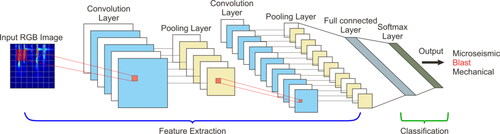
From the structure and training process of a CNN, the network is briefly described: the typical network structure of CNN is mainly composed of an input layer, convolution layers, pooling layers, fully connected layers, and a recognition layer (Figure 4). The convolution and pooling layers are adopted to extract features, while the fully connected and recognition layers are used for final recognition.

Figure 4. The typical network structure of the CNN.

3.2.1. Convolution layer

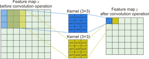
A convolution layer usually contains several feature planes, each composed of multiple neurons. Each neuron is obtained by convoluting the given convolution kernel, moving over a certain step with the local region of the feature plane in the upper layer (called local receptive field). The convolution kernel is a weight matrix, usually a 3 × 3 or 5 × 5 matrix in two-dimensional (2D) images (Gao et al. 2016). These convolution kernel functions act on the input images to extract local features therein. The convolution operation is shown in Figure 5. Different convolution kernels can extract different features, such as edges, lines, and corners of images, and the higher-level the convolution layer, the higher the level of feature extraction (Hinton 2010; Dahl et al. 2013). A new feature map can be generated by inputting the convolution result of the feature maps in the upper layer into the activation function.

Figure 5. Schematic diagram of the convolution operation. The left panel shows the feature map before convolution operation, and the right panel shows the feature map after convolution operation.

3.2.2. Pooling layer

The pooling layer lies below the convolution layer, and its function is to reduce the dimension of the feature maps based on retaining useful information and improving the calculation speed of the network. The combination of a convolution layer and a pooling layer is called a feature extraction process. The commonly seen pooling operations are averaging and maximum pooling. After pooling, the resolution of the feature map decreases, but the features described by the high-resolution feature maps are maintained (Simard et al. 2003).

3.2.3. Fully connected layer

Below multiple convolution layers and pooling layers, one or more fully connected layers are established. The purpose of the fully connected layer is to integrate the highly abstract features obtained from the convolution layer or pooling layer and then normalize them. Each neuron in the fully connected layer is connected to all neurons in the upper layer. In the pooling layer, the vectors of the feature map are a 2D array, which needs to be converted into 1D vectors, and then these 1D vectors are connected to form the input of the fully connected layer. Thus, the mathematical expression of a single neuron in the fully connected layer is given by: (13) $$\mathbf{Q}=\mathbf{f}({\mathbf{W}}^T\mathbf{X}\mathit{+}\mathbf{b})$$(13) where, Q represents the output of the obtained fully connected layer; f and b separately indicate the activation function and bias value; ${\mathbf{W}}^T$ denotes the weight to be trained; X denotes the eigenvector of the upper layer (pooling layer).

3.2.4. Regression layer

The output value of the last fully connected layer is transferred to the regression layer to realize recognition or regression calculation. The implementation process is shown in Figure 6. The part to the left of the equals sign in the figure is the work of the fully connected layer, which is the mathematical meaning described in Eq. (13)(13) $$\mathbf{Q}=\mathbf{f}({\mathbf{W}}^T\mathbf{X}\mathit{+}\mathbf{b})$$(13) . The matrix W is a parameter of the fully connected layer, an M × N matrix (where M is the number of classes). When training the network, the fully connected layer is used to find the most appropriate weight matrix W. As described in Eq. (13)(13) $$\mathbf{Q}=\mathbf{f}({\mathbf{W}}^T\mathbf{X}\mathit{+}\mathbf{b})$$(13) , the output of the fully connected layer is an M × 1 vector, i.e., Logits in Figure 6. For the multi-recognition problem, the fully connected layer is followed by a Softmax layer.

Figure 6. The implementation process of the Softmax layer.

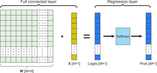
The idea for realizing the Softmax layer is as follows: for an input vector x, the conditional probability that the vector belongs to the jth class is first calculated, and then normalized so that the output probability lies on the range from 0 to 1, that is, Prob in Figure 6. Each value of such a vector represents the probability that the input sample belongs to each class. The output with the highest probability corresponds to the obtained class.

3.2.5. Training process

The training of CNN includes two processes, namely forward propagation and backward propagation. The above description of the structures of CNN follows the order of forwarding propagation. In the forwarding propagation, the signal input X in the first layer forms the output O of the last layer after multi-layer convolution, pooling, and feature integration in fully connected layers. The error C is calculated by comparing the output with the expected tag T, which is also known as the loss function, defined as follows: (14) $$C=\frac{1}{2n}{\sum _x\Vert y(x)-a\Vert }^2$$(14) where, n is the number of the samples, and the loss of all training samples is averaged; x and y(x) indicate the input of neutral network and predicted value corresponding to the input x, respectively; a represents the given tag.

In the training process, when the recognition result is inconsistent with expectations (that is, the final value is inconsistent with the expected value), the back-propagation (Girshick 2015) is conducted to calculate the error between the result and expected value. The backward paths of the neural network are traversed, and the error is back-transferred to each node on a layer-by-layer basis to calculate errors in each layer. Thereafter, the weight is updated. Based on the gradient of the least descent method, the weight and bias of the network are adjusted. Finally, the training ends when the loss function in the training samples is less than a specific threshold value. The final weight and bias are used for prediction and recognition.

3.3. LSTM model

LSTM model is composed of several typical LSTM units in series, and the structure of the LSTM unit is shown in Figure 7. The LSTM unit attempts to add or eliminate information for neurons by introducing the concept of a ‘gate’ that is (Graves 2012), controlling the input and output of information to realize the memory function. The LSTM unit contains three gates (input gate, output gate, and forget gate), which are used to protect and control the state of the storage cell C.

Figure 7. LSTM units and connection mode of forge gate, input gate and output gate.

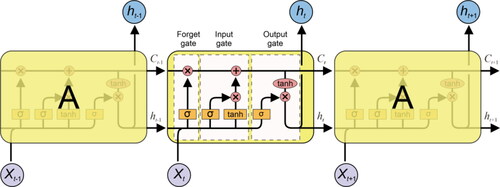
The forget gate aims to control how much information in the storage cell $C_{t-1}$ at the previous moment is to be kept in the storage cell $C_t$ at the current moment. The input gate mainly controls how much information on the input $X_t$ at the current moment is to be stored in the storage cell $C_t.$ The output gate is mainly used to control how much information in the storage cell $C_t$ at a certain moment is passed to the hidden state $h_t$ of the cell. In a forget gate, the forgotten part of a state memory cell is commonly determined by input $X_t,$ state memory cell $C_{t-1},$ and intermediate output $h_{t-1}.$ $X_t$ in an input gate transformed by sigmoid and tanh functions commonly determines the retaining vector in the state memory cell. The intermediate output $h_t$ is jointly determined by updated $C_t$ and output $O_t.$ The above working principle is exemplified by the following equations: (15) $$f_t=\sigma ({\mathbf{W}}_{fx}{X}_t+{\mathbf{W}}_{fh}{h}_{t-1}+b_f)$$(15) (16) $$i_t=\sigma ({\mathbf{W}}_{ix}{X}_t+{\mathbf{W}}_{ih}{h}_{t-1}+b_i)$$(16) (17) $$g_t=\varphi ({\mathbf{W}}_{gx}{X}_t+{\mathbf{W}}_{gh}{h}_{t-1}+b_g)$$(17) (18) $$O_t=\sigma ({\mathbf{W}}_{ox}{X}_t+{\mathbf{W}}_{oh}{h}_{t-1}+b_o)$$(18) (19) $$C_t=g_t\odot i_t+C_{t-1}\odot f_t$$(19) (20) $$h_t=\varphi (C_t)\odot O_t$$(20) where, $f_t,$ $i_t,$ $g_t,$ $O_t,$ $C_t,$ and $h_t$ separately represent the forget gate, input gate, input node, output gate, and memory cell and state of immediate output; ${\mathbf{W}}_{fx},$ ${\mathbf{W}}_{fh},$ ${\mathbf{W}}_{ix},$ ${\mathbf{W}}_{ih},$ ${\mathbf{W}}_{gx},$ ${\mathbf{W}}_{gh},$ ${\mathbf{W}}_{ox},$ and ${\mathbf{W}}_{oh}$ indicate the matrix weights of the corresponding gate multiplied by the input $X_t$ and intermediate output $h_{t-1},$ respectively; $b_f,$ $b_i,$ $b_g,$ and $b_o$ denote the bias terms of the corresponding gates; $\odot$ stands for that elements in the vector are subjected to bit-wise multiplication; $\sigma$ and $\varphi$ refer to the sigmoid and tanh functions, respectively.

In the LSTM model, several LSTM units receive the characteristic input of a monitoring signal at different moments. Through the above operation of three gates, the historical information of the time series can be recorded. At each moment, the attributes at the current and previous moments are recorded. Such a feature confers an important advantage when recognizing MS monitoring signals. In learning and training, the LSTM adopts the same back-propagation method for errors as used in CNN.

3.4. SSA-CNN-LSTM hybrid model

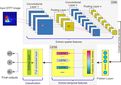
CNN and LSTM are the main algorithms used in deep learning, but they have advantages in dealing with different data types. CNN can extract high-level features with strong representational ability in spatial dimensions. On the other hand, LSTM can extend temporal features and is good at processing data from monitoring signals with sequence characteristics. The monitoring signal is transformed into a time-frequency map and input to the network in images. In the process, the spatial feature information and that pertaining to the time dimension should be considered. Based on the above features, in combination with the SSA method, CNN, and LSTM, the SSA-CNN-LSTM hybrid model was established by network series connection, which makes full use of the representational abilities of the CNN and LSTM for spatial and temporal features.

The structure of the SSA-CNN-LSTM hybrid model is shown in Figure 8. The principal components of monitoring signals are extracted by the SSA method. The essential parameters of the signals are obtained by STFT and converted into RGB images as input to the SSA-CNN-LSTM hybrid model. Then, they will be transferred in the convolution layer and pooling layer of CNN and hidden layer of LSTM networks to obtain an optimal feature representation. Finally, the monitoring signals are classified into corresponding classes using Softmax, a multi-class non-linear activation function in the fully connected layer.

Figure 8. The structure of CNN-LSTM hybrid networks. MS, M, and BL stand for MS signal, mechanical signal, and blasting signal, respectively.

4. Implementation process and result analysis of the SSA-CNN-LSTM

4.1. Implementation process of the SSA-CNN-LSTM

The detailed implementation steps of the SSA-CNN-LSTM hybrid model are summarized as follows, and the flowchart is shown in Figure 9:

Figure 9. The flow chart of the SSA-CNN-LSTM hybrid networks: (a) data pre-processing, (b) extract RC of signals by SSA method, (c) build signal recognition hybrid networks, and (d) test the signal recognition performance.

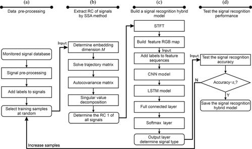
(1) Data pre-processing

The flowchart is shown in Figure 9(a):

• At first, all signals in the signal database are pre-processed to ensure three types of signals (MS, blasting, and mechanical signals) have the same length by upper and lower sampling methods.

• Afterwards, the corresponding labels, MS signal label, blasting signal label, or mechanical signal label, are assigned to the monitoring signals in the signal database.

• The 70% data are stochastically taken from the monitoring signal database as the training samples, and the other 30% data are as the validation samples.

(2) Extract RCs of the signals by the SSA method

The flowchart is shown in Figure 9(b):

• At first, the method proposed by Cao (1997) is used to determine an appropriate embedding dimension. Subsequently, a trajectory matrix is constructed; the autocovariance matrix is solved, and the singular value decomposition is performed.

• Afterwards, save the RC 1 of all signals from the training samples.

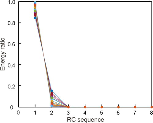
To determine the number K of RCs, 30 MS signals were randomly selected from the signal database for analysis. Figure 10 shows the SSA analysis process of a randomly selected signal among the 30 MS signals. Figure 10(b) shows the first five principal RCs: the amplitude of the RC 1 is high, at about ten times that of RC 2. The MS signal amplitudes gradually reduce from RC 2 to RC 5, in which the amplitude of RC 1 is about 1000 times that of RC 5 (RC 3 to RC 5 contain significant noise). Figure 10(c) shows the energy ratio of RCs to the original MS signal. According to the principle that the energy of a valid signal component is higher than that of noise in MS signals, it can be thought that RC 1 is the valid component of the MS signal, and the signals are reconstructed from the rest of the singular values are noise. By comparing RC 1 with the original MS signal (Figure 10(d)), valid MS signal components are retained in RC 1. The energy ratio of RCs to the original MS signal of the 30 MS signals is solved, as shown in Figure 11. Figure 11 shows that the energy ratios of the RC 1 of the 30 random MS signals are far larger than those of the other RCs; that is, the valid components of signals are concentrated on RC 1. Therefore, in this step, the K is taken as 1 to meet the requirements.

Figure 10. SSA analysis process of the MS signal with severe noise: (a) original MS signal, (b) RC 1–RC 6, (c) energy ratio of RCs to the original MS signal, and (d) comparison of RC 1 and original MS signal.

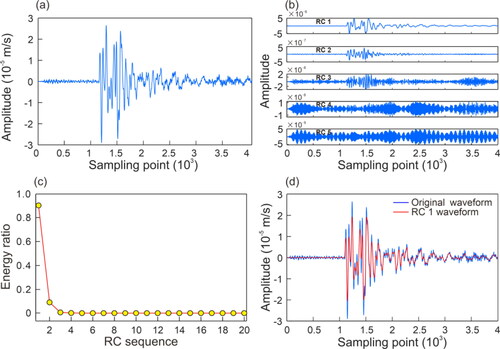
Figure 11. Energy ratio of each RC of 30 MS signals. 1 to 8 in the horizontal axis represent the first to eighth RC of the MS signal.

(3) Build the signal recognition hybrid networks

The flowchart is shown in Figure 9(c):

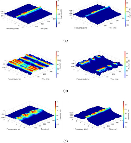
• RC 1 of all signals of the training samples is subjected to the STFT method for attaining the time-frequency map, which contains time, frequency, and amplitude characteristics of signals. This time-frequency map is used as the input of the hybrid networks.

For example, Figure 12 shows the STFT results of MS, blasting, and mechanical signals (Figure 2) before and after extracting effective components through the SSA method: the time-frequency characteristics of the three signals are largely different. Specifically, the frequency of MS signals is lower and more concentrated, and the signals attenuate slowly. The time-frequency maps of mechanical and MS signals demonstrate that their frequencies are concentrated within the same range and have similar amplitudes; however, their time-frequency maps show that mechanical signals attenuate more slowly than MS signals. After the signals are processed by the SSA method, the signals can be better distinguished. Using the STFT program, the time, frequency, and amplitude characteristics of signals can be considered by STFT without the need for multi-parameter extraction, as is the case when using conventional methods.

Figure 12. Time-frequency amplitude diagrams of three typical monitoring signals before and after tht SSA processing: (a) MS signal, (b) blasting signal, and (c) mechanical signal.

• Design the hybrid model structure

The networks structure of SSA-CNN-LSTM is complex, so the optimal results can only be found through trial and error. Several trials with different structures were conducted, and the final SSA-CNN-LSTM topological structure is shown in Figure 13 and Table 1.

Figure 13. The network structure of the proposed CNN-LSTM hybrid model.

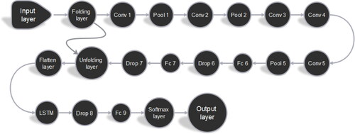
Table 1. The network structure of the SSA-CNN-LSTM hybrid networks model.

Number of layers	Layer type	Activation function	Output size	Number and size of convolution kernels
1	Input layer		227 × 227 × 3
2	Folding layer		227 × 227 × 3
3	Convolution layer (Conv 1)	ReLU	55 × 55 × 96	96, 11 × 11
4	Maximum pool layer (Pool 1)		27 × 27 × 96	96, 3 × 3
5	Convolution layer (Conv 2)	ReLU	27 × 27 × 256	256, 5 × 5
6	Maximum pool layer (Pool 2)		13 × 13 × 256	256, 3 × 3
7	Convolution layer (Conv 3)	ReLU	13 × 13 × 384	384, 3 × 3
8	Convolution layer (Conv 4)	ReLU	13 × 13 × 384	384, 3 × 3
9	Convolution layer (Conv 5)	ReLU	13 × 13 × 256	256, 3 × 3
10	Maximum pool layer (Pool 5)		6 × 6 × 256	256, 3 × 3
11	Full connection layer (Fc 6)	ReLU	1 × 1 × 4096
12	Dropout layer (Drop 6)		1 × 1 × 4096
13	Full connection layer (Fc 7)	ReLU	1 × 1 × 4096
14	Dropout layer (Drop 7)		1 × 1 × 4096
15	Unfolding layer		1 × 1 × 4096
16	Flatten layer		4096
17	LSTM		4000
18	Dropout layer (Drop 8)		4000
19	Full connection layer (Fc 9)		3
20	Softmax layer	Softmax	3
21	Output layer

The first layer of the SSA-CNN-LSTM is the input layer, whose input is the time-frequency RGB image generated in the above steps. Use a sequence folding layer to perform convolution operations on time steps of image sequences independently. There are five convolution layers from the third to the seventh layer in the network structure, coupled with the maximum pooling layer. Fc 6 and Fc 7 in Table 1 are fully connected layers. An unfolding layer and a flatten layer are connected behind them for restoring the sequence structure and reshape the output to vector sequences. Then, the reshape vector sequence is input into the LSTM layer. In the final stage of the hybrid networks model, one fully connected layer and a Softmax layer are used for signal recognition and output. In addition, three dropout operations (take 0.5) are used in the whole hybrid networks to reduce the possibility of overfitting and improve the model's generalization ability.

There are many hyperparameters to be tested in such a deep neural network, including the learning factor α, factor β of gradient descent with momentum, parameters (β₁, β₂, and ε) of the Adam optimization algorithm, descent parameters of learning factor, and the number of samples contained in batch training samples. In this study, the learning factor α was set to 0.001 and the three parameters β₁, β₂, and ε in the Adam algorithm were set to 0.9, 0.999, and 10⁻⁶, respectively.

(4) Test the recognition performance

The flowchart is shown in Figure 9(d):

• The validation samples are input; the signal recognition is performed with the aid of the SSA-CNN-LSTM hybrid model trained through the aforementioned steps, and then the result is compared with that obtained through manual signal recognition.

• The threshold ${\epsilon }_1$ of the signal recognition accuracy is set (90% in this article). That is, if the accuracy of the signal recognition is more than 90%, then the SSA-CNN-LSTM hybrid model satisfies the requirement and is preserved; otherwise, the model is further trained with increasing training samples until it satisfies the requirement.

4.2. Result analysis

4.2.1. Signal recognition performance using conventional recognition methods

This section aims to test the recognition performance of the conventional recognition methods based on characteristic parameters of signals for the three types of signals and compare these with the SSA-CNN-LSTM to highlight the necessity for this article.

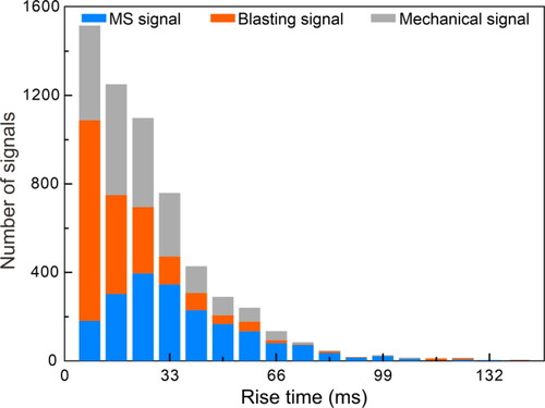
By calculating parameters of the three types of signals in the signal database many times and referring to the results of references (Dong et al. 2016b; Li et al. 2018), four parameters were determined as characteristic parameters for signal recognition. These include the number of signal peaks (reflects the number of signals released in a short time), the dominant frequency (reflects the essential characteristics of the signal), and the maximum amplitude (reflects the intensity of signal), and the rise time (reflects the energy rate of the signal in a short time, which is related to rock failure). The rise time is defined as the time from P-wave onset to the maximum amplitude of the MS signal. The modified STA/LTA method (https://ww2.mathworks.cn/matlabcentral/fileexchange/51996-suspension-bridge-picking-algorithm-sbpx?s_tid=srchtitle.) is used for picking the P-wave onset.

Figures 3 and 14 show the distribution of four characteristic parameters of the three types of signals. As demonstrated in Figure 3(a), MS signals with a small dominant frequency are easily distinguished from blasting signals. However, MS and mechanical signals overlap in low-frequency band, so it is not easy to distinguish them based on this parameter. It can be seen from Figure 3(b) that MS signals mainly have one peak. On the other hand, the mechanical signals and blasting signals have multi-peak characteristics. Therefore, the number of peaks can distinguish MS signals from blasting and mechanical signals, but it is not easy to distinguish blasting signals from mechanical signals. As displayed in Figure 3(c), for the maximum amplitude, MS and mechanical signals can be easily distinguished from blasting signals. In contrast, MS signals and mechanical signals are not easy to distinguish based on this parameter. It can be observed from Figure 14 that the rise time of MS signals is longer than the other two signals. However, these three kinds of signals still have more overlap in this parameter. In conclusion, it is not easy to distinguish the three types of signals with a single parameter, so it is necessary to use multiple parameters for comprehensive recognition.

Figure 14. The rise time of three kinds of signals.

According to the four characteristic parameters in Figures 3 and 14, the recognition of MS signals are classified as an indistinguishable linear problem. In this section, four commonly used recognition models, namely the SVM (Suykens and Vandewalle 1999), decision tree (DT) (Safavian and Landgrebe 1991), K-nearest neighbor (KNN) (Keller et al. 1985), and linear discriminant analysis (LDA) (Chengjun and Wechsler 2002), were used for preliminary assessment of the recognition accuracy of such signals. To determine accurate recognition results, the 5-fold cross-validation method was used to train the four recognition models. The recognition performance of the total and the individual of the four models are shown in Table 2. Figure 15 shows the confusion matrix of the four models taking the mean performance of five tests. It can be observed from Figure 15 and Table 2 that by using the SVM method, the recognition rate of MS signals is the highest (92.34%), followed by that of blasting signals (89.16%). In comparison, the recognition rate of mechanical signals is only 73.6%. The DT, KNN, and LDA methods are ranked in descending order according to the recognition effect. Their recognition accuracies for MS, blasting, and mechanical signals are lower than that of the SVM method. Therefore, when MS signals are recognized based on characteristic parameters of waveforms, higher accuracy can be obtained by using the SVM method.

Figure 15. Confusion matrices of recognition results of four commonly used methods: (a) SVM, (b) KNN, (c) DT, (d) LDA. MS, M, and BL stand for MS signal, mechanical signal, and blasting signal.

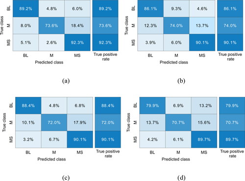
Table 2. Signal recognition accuracy for four conventional methods using 5-fold cross-validation.

Models	Category	1st test	2nd test	3rd test	4th test	5th test	Mean
SVM	MS signal	92.1%	91.6%	92.2%	93.4%	92.4%	92.34%
	Blasting signal	88.2%	89.2%	89.3%	90.6%	88.5%	89.16%
	Mechanical signal	72.8%	74.4%	73.2%	75.0%	72.6%	73.6%
	Total	84.37%	85.07%	84.90%	86.33%	84.50%	85.03%
KNN	MS signal	90.1%	89.1%	91.2%	90.4%	89.7%	90.1%
	Blasting signal	85.2%	86.3%	87.1%	85.1%	86.6%	86.06%
	Mechanical signal	74.8%	74.6%	73.1%	73.2%	74.1%	73.96%
	Total	83.37%	83.33%	83.80%	82.90%	83.47%	83.37%
DT	MS signal	89.1%	89.4%	91.0%	89.5%	91.6%	90.12%
	Blasting signal	88.7%	87.6%	88.1%	90.1%	87.5%	88.4%
	Mechanical signal	71.5%	74.2%	70.6%	71.1%	72.3%	71.94%
	Total	83.10%	83.73%	83.23%	83.57%	83.80%	83.49%
LD	MS signal	89.6%	90.2%	88.4%	90.6%	89.9%	89.74%
	Blasting signal	80.5%	78.9%	81.1%	79.6%	79.4%	79.9%
	Mechanical signal	69.5%	70.6%	71.4%	71.8%	70.2%	70.7%
	Total	79.87%	79.90%	80.30%	80.67%	79.83%	80.11%

Meanwhile, it is not difficult to see from Figure 15 that the SVM method has certain limitations. The method has a low recognition rate for mechanical signals, and 18.4% of mechanical signals will be recognized as MS signals, affecting MS data processing. Because of this, a new recognition model for MS signals needs to be established to overcome such limitations.

4.2.2. Signal recognition performance using SSA-CNN-LSTM hybrid model

Similarly, to determine accurate recognition results and validate the SSA-CNN-LSTM hybrid model, the 5-fold cross-validation method was also used to train the SSA-CNN-LSTM hybrid model. As a result, the recognition performance of the total and the individual is shown in Table 3. Besides, to verify the recognition performance of the SSA-CNN-LSTM model compared with other network models, the 5-fold cross-validation of the single CNN, the single LSTM, and BP is also carried out, and the results are listed in Table 3. For details of BP network structure and parameter setting, please refer to the literature (Xu et al. 2021). The input to the single CNN is the time-frequency RGB image transformed by the STFT method from the original monitoring signal (Figure 12). The input to the single LSTM and BP networks is the time-frequency series transformed by the STFT method.

Table 3. Signal recognition accuracy for four neural network methods using 5-fold cross-validation.

Models	Category	1st test	2nd test	3rd test	4th test	5th test	Mean	Standard deviation
SSA-CNN-LSTM	MS signal	97.8%	96.3%	97.3%	97.4%	97.3%	97.2%	0.49
	Blasting signal	95.3%	94.4%	93.2%	93.3%	93.8%	94.0%	0.78
	Mechanical signal	92.8%	93.3%	92.5%	91.8%	92.0%	92.5%	0.54
	Total	95.3%	94.67%	94.3%	94.17%	94.37%	94.56%	0.40
CNN	MS signal	94%	93.8%	95.5%	94.8%	93.5%	94.32%	0.73
	Blasting signal	93.5%	93.0%	90.5%	91.0%	92.8%	92.16%	1.18
	Mechanical signal	89.5%	88.5%	90.3%	86.9%	90.8%	89.2%	1.39
	Total	92.33%	91.77%	92.10%	90.90%	92.37%	91.96%	0.54
LSTM	MS signal	92.5%	93%	94.3%	93.8%	94.1%	93.54%	0.68
	Blasting signal	90.8%	89.3%	87.8%	88.3%	89.5%	89.14%	1.04
	Mechanical signal	86.3%	86.1%	84.2%	88.8%	87.0%	86.48%	1.49
	Total	89.87%	89.47%	88.77%	90.3%	90.2%	89.72%	0.56
BP	MS signal	89.2%	87.4%	88.8%	87.2%	88.3%	88.18%	0.78
	Blasting signal	86.6%	83.3%	86.4%	83.3%	86.3%	85.18%	1.54
	Mechanical signal	81.9%	74.0%	77.9%	77.0%	75.9%	77.34%	2.62
	Total	85.90%	81.57%	84.37%	82.50%	83.50%	83.57%	1.50

It can be seen from Table 3 that the standard deviation of recognition performance of the SSA-CNN-LSTM of the total and individual using fivefold cross-validation is smaller than other networks. That is to say, the recognition performance of the SSA-CNN-LSTM proposed in this article is stable. The stability of recognition performance of the LSTM is slightly higher than that of the CNN, but both are better than the BP. In addition, it is easy to find out from Table 3 that the signal recognition accuracy of the SSA-CNN-LSTM is significantly higher than those of the single CNN, the single LSTM, and BP. The total recognition accuracy of the single CNN and single LSTM networks reaches 89.72% and 91.96%, respectively, and the recognition performance of MS signal is more than 90%. It shows that CNN has an excellent ability to extract spatial features from time-frequency RGB images. LSTM have an excellent ability to extract temporal features during feature extraction from time-series data. By comparing the recognition performance of the network models, the SSA-CNN-LSTM can better integrate the advantages of CNN and LSTM. In addition, the recognition performance of the BP is the worst among the four networks. It is proved that the feature extraction ability of deep learning is better than that of a traditional neural network.

To compare the recognition performance of these four models in more detail, Figure 16 shows the confusion matrix of the four models taking the mean performance of 5 tests. Meanwhile, the recognition performance of SSA-CNN-LSTM, CNN, LSTM, BP networks were compared with SVM, KNN, DT, and LDA, and the results are displayed in Figure 17.

Figure 16. Confusion matrices of recognition results of four neural network methods: (a) SSA-CNN-LSTM, (b) CNN, (c) LSTM, and (d) BP.

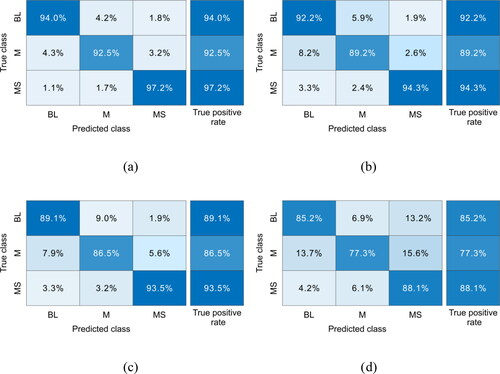
Figure 17. Comparison of signal recognition accuracy of eight methods.

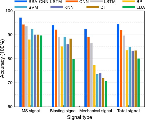
By analyzing Figures 16 and 17, it is concluded that the total recognition accuracy of the SVM method with the best recognition accuracy in Section 4.2.1 is only 85.03%. In comparison, the SSA-CNN-LSTM is improved by 9.53%. In addition, it can be observed from the confusion matrix of the SSA-CNN-LSTM that the recognition accuracy of blasting and MS signals are excellent, with recognition accuracy exceeding 94%. In addition, as described in Section 4.2.1, owing to the similarity of the MS and mechanical signals, the recognition performance of the two type signals is lacking: the recognition accuracies for mechanical signals with the SVM, DT, KNN, and LDA methods are only 73.6%, 72.0%, 74.0%, and 70.7%, respectively. In contrast, the recognition accuracies for mechanical signals with the CNN and LSTM rise to 89.2% and 86.5%, while that arising from the use of the SSA-CNN-LSTM is 92.5%, that is, only 3.2% of mechanical signals will be mistaken for MS signals. Thus, the recognition accuracy of the SSA-CNN-LSTM is improved significantly.

The SSA-CNN-LSTM hybrid model proposed in this research considers the spatial and temporal features simultaneously, which is excellent for signal recognition. It can recognize MS signals required for the research from the monitoring signals in a complex underground environment and meet practical application needs in Xiadian Gold Mine.

5. Discussion

A new hybrid signal recognition model—SSA-CNN-LSTM for MS monitoring in underground mines was proposed. The SSA-CNN-LSTM integrates the advantages of local spatial feature extraction of CNN, the advantages of temporal feature extraction of LSTM, and the ability of principal component extraction of SSA method, and achieves a good recognition performance of three types of signals. Compared with conventional methods and a single depth network model, it has a higher recognition performance and better stability.

The number of the three types of samples studied above is balanced. When the number of three types of samples is imbalanced, the recognition accuracy needs to be tested. Therefore, the MS, blasting, and mechanical signals were set to different proportions, with nine proportions. The grouping results are shown in Tables A1 and A2 in Appendix A. To meet the calculation requirements, the number of some samples in Table A1 exceeds the number of measured signals. In this case, resampling is used to increase samples. The SSA-CNN-LSTM was used to test the recognition performance of the sample distribution described in Tables A1 and A2. The test results are shown in Tables A3 and A4. The test results show that the sample's distribution has a significant impact on the recognition performance of the SSA-CNN-LSTM. It can be seen from ID 8 and ID 9 in Tables A3 and A4 that mechanical signal is most significantly affected by the number of samples. It shows that the mechanical signal has a strong similarity with the MS signal, so it needs more training samples to ensure the recognition performance. On the contrary, from ID 3 and ID 7 in Table A3, it can be found that even if the number of MS signals is reduced to 1000, the recognition accuracy can still maintain more than 90%. Thus, to achieve the ideal recognition accuracy, different types of signals need a different number of training data. To achieve a higher total recognition performance, the samples with a lower proportion can be supplemented by resampling. As shown from Figure A1, using the oversampling on the imbalanced data can increase the SSA-CNN-LSTM performances to that of the SSA-CNN-LSTM trained with balanced data.

As can be seen from Figure 16(a), in the case of sample balance, although the recognition accuracy of MS signals reaches 97.2%, there are still 5.0% other signals that will be mistaken for MS signals, and the recognition model needs to be further improved. For the underground mine site, many factors are affecting the recognition performance of MS signals. For example, MS signals are usually mixed with other types of signals, which will change the frequency and amplitude characteristics of MS signals. Therefore, an excellent pre-processing method is an essential factor in improving the recognition performance, which is as important as the recognition model.

The pre-processing method of the SSA-CNN-LSTM has experienced the components extraction and STFT transformation, which takes a long time. At the same time, due to the introduction of LSTM, compared with the single CNN, the training time of the model is also increased. In addition, due to the complexity of the monitoring signals, it takes a long time to screen the monitoring signals manually. 7164 signals used in this article were processed for 15 days. Therefore, to ensuring the recognition performance, the model with fewer training samples is very important for processing mine MS monitoring signals. A more advanced CNN or LSTM network may further improve the recognition performance while reducing the training time and required training samples.

The network structural parameters of the SSA-CNN-LSTM are determined by the trial-and-error method. There is no mature theory to give the number of required network layers and neurons quantitatively. In this study, the same network structural parameters for the SSA-CNN-LSTM were used for all tests, and different results may be obtained with other parameters. Furthermore, due to the complexity of the mine environment, the network structure in this study is not necessarily suitable for other mines. Therefore, the SSA-CNN-LSTM needs to be adjusted when it is applied in other mines.

6. Conclusion

1. A new hybrid networks model—SSA-CNN-LSTM based on SSA, CNN, and LSTM is proposed. This hybrid networks model combines signal principal component extraction, local spatial feature extraction, and temporal feature extraction. It provides a new idea for the effective recognition of MS monitoring signals

2. Based on the actual monitoring data recorded in the Xiadian Gold Mine, the monitoring signals are recognized by four commonly used methods, i.e., SVM, DT, KNN, and LDA. It is found that the recognition accuracy obtained by SVM is best among those four methods and its recognition accuracy for MS signals reaches 92.3%. However, the recognition accuracy of SVM for mechanical signals is only 73.6%, and 18.4% of mechanical signals will be mistaken for MS signals, which is too inaccurate to allow in situ practical application.

3. The proposed SSA-CNN-LSTM hybrid model is tested and compared with the CNN, LSTM, BP models, and four commonly used methods: the total recognition accuracy of the SSA-CNN-LSTM hybrid model increased to 94.56%. Furthermore, the individual recognition accuracies for MS, blasting, and mechanical signals reached 97.2%, 94.0%, and 92.5%, respectively. Therefore, only 3.2% of mechanical signals are mistaken for MS signals, indicating that recognition performance is further improved than other methods.

Disclosure statement

No potential conflict of interest was reported by the authors.

Data availability statement

The data that support the finding of this study are available from the corresponding author upon reasonable request.

Additional information

Funding

This work was supported by the National Natural Science Foundation of China (U1710253 and 52004052), Post-doctoral International Exchange Program (2020059), Post-doctoral fund of Northeastern University (20200202), and the Fundamental Research Funds for the Central Universities (N2101027 and N180701005).

Appendix A

Figure A1. The total performance of each distribution with and without over-sampling from Table A2 and Table A5. ID 1 shows no result after oversampling since it was already balanced.

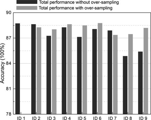
Table A1. Nine distributions of 6000 signals for researching on the impact of imbalanced training data for the SSA-CNN-LSTM model.

ID	MS signals	Blasting signal	Mechanical signal
1	2000	2000	2000
2	1500	2500	2000
3	1000	3000	2000
4	2500	1750	1750
5	3000	1500	1500
6	1500	2250	2250
7	1000	2500	2500
8	2500	2500	1000
9	2250	2250	1500

Table A2. Nine distributions of 3000 signals for researching on the impact of imbalanced training data for the SSA-CNN-LSTM model.

ID	MS signals	Blasting signal	Mechanical signal
1	1000	1000	1000
2	750	1250	1000
3	500	1500	1000
4	1250	875	875
5	1500	750	750
6	750	1125	1125
7	500	1250	1250
8	1250	1250	500
9	1125	1125	750

Table A3. The total and the individual recognition accuracies (the total number of samples is 6000).

ID	MS signals	Blasting signal	Mechanical signal	Total
1	97.2%	94.0%	92.5%	94.57%
2	94.7%	92.9%	91.0%	92.87%
3	94.1%	95.1%	93.0%	94.07%
4	96.0%	89.0%	89.8%	91.60%
5	96.4%	84.4%	88.0%	89.60%
6	94.9%	92.2%	93.9%	93.67%
7	91.6%	94.3%	95.0%	93.63%
8	96.8%	94.5%	79.2%	90.17%
9	96.3%	92.3%	85.9%	91.50%

Table A4. The total and the individual recognition accuracies (the total number of samples is 3000).

ID	MS signals	Blasting signal	Mechanical signal	Total
1	92.1%	86.6%	87.5%	88.73%
2	91.8%	87.0%	87.1%	88.63%
3	85.0%	90.3%	86.5%	87.27%
4	92.0%	85.6%	87.2%	88.27%
5	93.3%	81.3%	86.8%	87.13%
6	90.3%	87.7%	86.2%	88.07%
7	87.0%	88.6%	88.1%	87.90%
8	91.2%	90.4%	73.0%	84.87%
9	91.8%	86.4%	78.0%	85.40%

Table A5. The total and the individual recognition accuracies with oversampling (the total number of samples is 3000).

ID	MS signals	Blasting signal	Mechanical signal	Total
2	92.1%	86.6%	87.5%	88.73%
3	91.2%	86.5%	87.1%	88.27%
4	90.5%	87.1%	86.5%	88.03%
5	91.5%	86.3%	88.1%	88.63%
6	91.9%	86.5%	87.1%	88.50%
7	90.4%	87.5%	88.4%	88.77%
8	91.0%	87.0%	90.1%	89.37%
9	91.1%	86.5%	84.8%	87.47%

ID 1 is not included since it was already balanced and thus was not oversampled.

References

- Abdel-Hamid O, Mohamed A, Jiang H, Deng L, Penn G, Yu D. 2014. Convolutional neural networks for speech recognition. IEEE/ACM Trans Audio Speech Lang Process. 22(10):1533–1545.
- Alex K, Sutskever I, Hinton GE. 2012. ImageNet classification with deep convolutional neural networks. In: Advances in neural information processing systems. Curran Associates, Inc Lake Tahoe, NV, United States. p. 1097–1105.
- Allmann BP, Shearer PM, Hauksson E. 2008. Spectral discrimination between quarry blasts and earthquakes in Southern California. Bull Seismological Soc Am. 98(4):2073–2079.
- Arrowsmith SJ, Arrowsmith MD, Hedlin MAH, Stump B. 2006. Discrimination of delay-fired mine blasts in Wyoming using an automatic time-frequency discriminant. Bull Ssmological Soc Am. 96(6):2368–2382.
- Backers T, Stanchits S, Dresen G. 2005. Tensile fracture propagation and acoustic emission activity in sandstone: The effect of loading rate. Int J Rock Mech Mining Sci. 42(7–8):1094–1101.
- Bengio Y. 2009. Learning deep architectures for AI. FNT Mach Learn. 2(1):1–127.
- Cao L. 1997. Practical method for determining the minimum embedding dimension of a scalar time series. Phys D. 110(1–2):43–50.
- Chengjun L, Wechsler H. 2002. Gabor feature based classification using the enhanced fisher linear discriminant model for face recognition. IEEE Trans Image Process. 11(4):467–476.
- Dahl GE, Sainath TN, Hinton GE. 2013. Improving deep neural networks for LVCSR using rectified linear units and dropout. Proceedings of the IEEE International Conference on Acoustics. 26-31 May. Vancouver, BC, Canada.
- Dai F, Li B, Xu N, Zhu Y. 2017. Microseismic early warning of surrounding rock mass deformation in the underground powerhouse of the Houziyan hydropower station, China. Tunnelling Underground Space Technol. 62:64–74.
- Dong LJ, Li XB, Xie GN. 2014. Nonlinear methodologies for identifying seismic event and nuclear explosion using random forest, support vector machine, and naive Bayes classification. Abstr Appl Anal. 2014(459137):1–8.
- Dong LJ, Tang Z, Li XB, Chen YC, Xue JC. 2020. Discrimination of mining microseismic events and blasts using convolutional neural networks and original waveform. J Cent South Univ. 27(10):3078–3089.
- Dong LJ, Wesseloo J, Potvin Y, Li XB. 2016a. Discrimination of mine seismic events and blasts using the Fisher classifier, naive Bayesian classifier and logistic regression. Rock Mech Rock Eng. 49(1):183–211.
- Dong LJ, Sun DY, Li XB, Ma J, Chen GJ, Zhang CX. 2016b. A statistical method to identify blasts and microseismic events and its engineering application. Chin J Rock Mech Eng. 35:1423–1433. (in Chinese).
- Gao L, Chen PY, Yu S. 2016. Demonstration of convolution kernel operation on resistive cross-point array. IEEE Electron Device Lett. 37(7):870–873.
- Girshick R. 2015. Fast R-CNN. Proceedings of the IEEE International Conference on Computer Vision. 7-12 December. Santiago, Chile.
- Graves A. 2012. Long short-term memory. In: Supervised sequence labelling with recurrent neural networks. Berlin, Heidelberg: Springer Berlin Heidelberg; p. 37–45.
- Graves A, Jaitly N. 2014. Towards end-to-end speech recognition with recurrent neural networks. Proceedings of the International Conference on Machine Learning. 21-26 June. Beijing, China.
- Groth A, Ghil M. 2015. Monte Carlo singular spectrum analysis (SSA) revisited: detecting oscillator clusters in multivariate datasets. J Climate 28(19):7873–7891.
- Gu J, Wang Z, Kuen J, Ma L, Shahroudy A, Shuai B, Liu T, Wang X, Wang G, Cai J, et al. 2018. Recent advances in convolutional neural networks. Pattern Recognit. 77:354–377.
- Hensman P, Masko D. 2015. The impact of imbalanced training data for convolutional neural networks. KTH Computer Science and Communication. Stockholm, Sweden.
- Hinton GE. 2010. Rectified linear units improve restricted Boltzmann machines. Proceedings of the International Conference on International Conference on Machine Learning. 21 June. Haifa, Israel.
- Jian Z, Xu C, Zhang Z, Li X. 2017. Electric load forecasting in smart grids using long-short-term-memory based recurrent neural network. Proceedings of the Information Sciences & Systems. 22-24 March. Baltimore, MD, USA.
- Keller JM, Gray MR, Givens JA. 1985. A fuzzy K-nearest neighbor algorithm. IEEE Trans Syst Man Cybern. SMC-15(4):580–585.
- Kiranyaz S, Ince T, Gabbouj M. 2016. Real-time patient-specific ECG classification by 1-D convolutional neural networks. IEEE Trans Biomed Eng. 63(3):664–675.
- Kong WC, Dong ZY, Jia Y, Hill DJ, Xu Y, Zhang Y. 2019. Short-term residential load forecasting based on LSTM recurrent neural network. IEEE Trans Smart Grid. 10(1):841–851.
- Li CW, Sun XY, Gao TB, Xie BJ, Xu XM. 2015. Coal and rock vibration failure and the characteristics of micro-seismic signals. Jounal of China Coal Society. 40:1834–1844.
- Li XL, Li ZH, Wang EY, Liang YP, Li BL, Chen P, Liu YJ. 2018. Pattern recognition of mine microseismic and blasting events based on wave fractal features. Fractals. 26(03):1850029.
- Lv ZB, Ao CY, Zou Q. 2019. Protein function prediction: From traditional classifier to deep learning. Proteomics 19:1900119.
- Ma J, Zhao GY, Dong LJ, Chen GH, Zhang CX. 2015. A comparison of mine seismic discriminators based on features of source parameters to waveform characteristics. Shock Vib. 2015:1–10.
- Ma XL, Tao ZM, Wang YH, Yu HY, Wang YP. 2015. Long short-term memory neural network for traffic speed prediction using remote microwave sensor data. Transport Res C. 54:187–197.
- Pu YY, Apel DB, Liu V, Mitri H. 2019. Machine learning methods for rockburst prediction-state-of-the-art review. Int J Mining Sci Technol. 29(4):565–570.
- Quang PB, Gaillard P, Cano Y, Ulzibat M. 2015. Detection and classification of seismic events with progressive multi-channel correlation and hidden Markov models. Comput Geosci. 83:110–119.
- Safavian SR, Landgrebe D. 1991. A survey of decision tree classifier methodology. IEEE Trans Syst Man Cybern. 21(3):660–674.
- Simard P, Steinkraus D, Platt JC. 2003. Best practices for convolutional neural networks applied to visual document analysis. Proceedings of the International Conference on Document Analysis & Recognition. 6 August. Edinburgh, UK.
- Singh SK, Raval S, Banerjee B. 2021. A robust approach to identify roof bolts in 3D point cloud data captured from a mobile laser scanner. Int J Mining Sci Technol. 31(2):303–312.
- Sokolic J, Giryes R, Sapiro G, Rodrigues MRD. 2017. Robust large margin deep neural networks. IEEE Trans Signal Process. 65(16):4265–4280.
- Suykens JAK, Vandewalle J. 1999. Least squares support vector machine classifiers. Neural Process Lett. 9(3):293–300.
- Vallejos JA, McKinnon SD. 2013. Logistic regression and neural network classification of seismic records. Int J Rock Mech Min. 62:86–95.
- Vautard R, Ghil M. 1989. Singular spectrum analysis in nonlinear dynamics, with applications to paleoclimatic time series. Phys D. 35(3):395–424.
- Xu S, Liang RY, Suorineni FT, Li YH. 2021. Evaluation of the use of sublevel open stoping in the mining of moderately dipping medium-thick orebodies. Int J Mining Sci Technol. 31(2):333–346.
- Xu XF, Dou LM, Lu CP, Zhang YL. 2010. Frequency spectrum analysis on micro-seismic signal of rock bursts induced by dynamic disturbance. Mining Sci Technol. (China). 20(5):682–685.
- Xue QF, Wang YB, Chang X. 2016. Fast 3D elastic micro-seismic source location using new GPU features. Phys Earth Planet Int. 261:24–35.
- Zhang H, Ma CC, Pazzi V, Li TB, Casagli N. 2020. Deep convolutional neural network for microseismic signal detection and classification. Pure Appl Geophys. 177(12):5781–5717.
- Zhao Y, Yang T, Zhang P, Xu H, Zhou J, Yu Q. 2019. Method for generating a discrete fracture network from microseismic data and its application in analyzing the permeability of rock masses: A case study. Rock Mech Rock Eng. 52:3133–3155.
- Zhao Y, Yang TH, Zhang PH, Xu HY, Wang SH. 2020. Inversion of seepage channels based on mining-induced microseismic data. Int J Rock Mech Min. 126:104180.
- Zhigljavsky A. 2010. Singular spectrum analysis for time series: Introduction to this special issue. Statistics and Its Interface. 3(3):255–258.