A holistic view of Shisper Glacier surge and outburst floods: from physical processes to downstream impacts

Abstract

We observed the surge velocity, terminus advance, lake formation and outburst, as well as its downstream impacts at Shisper Glacier in the Karakoram, Pakistan and suggest potential nature-based risk-reduction solutions. A recent surge started in late 2017 with increased velocity since April 2018 and a resulting terminus advance from June 2018. Bi-modal peak velocity of 19.2 ± 0.16 m/day was observed in April-May 2018 and May-June 2019. Also, the terminus advance blocked the river from the adjacent Muchuhar Glacier repeatedly since November 2018. Lake outbursts were observed in June 2019 and April 2020. Relying on observations of the lake area and peak discharge of 142 m³ s⁻¹ in 2019 and 85 m³ s⁻¹ April 2020, outburst were simulated using the BASEMENT software. Simulations and field observations show that even at high discharge, damages were mainly observed along the main river channel, causing strong bank erosion rather than widespread inundation of land. The ice-dammed lake is potentially hazardous until the blocked stream completely disappears in future. Our results suggest that the biggest lake outburst hazard lies in its erosion potential with damages to infrastructure closest to the river and large sediments transport to the downstream Hunza River.

Keywords:

• Glacier surges
• GLOF
• remote sensing
• Shisper Glacier
• Karakoram

Introduction

Karakoram is the most heavily glacierized mountain range in Asia comprising ∼ one-fourth of the glaciers in the Himalaya-Karakoram-Hindukush (HKH) region (RGI Consortium 2017). The concentration of surge-type glaciers in the Karakoram is among the highest on Earth, spreading over ∼40% of the total glacier cover area (Hewitt 2014, Hewitt 1998; Bhambri et al. 2017), while globally 2317 equivalent to ∼1-2% of all glaciers have been observed to surge (Jiskoot et al. 1998; Sevestre and Benn 2015). During the surge phase, flow velocities increase by 10 to 100 times compared to the quiescent phase and the surge cycle lasts between weeks to years (Meier and Post 1969; Jiskoot 2011). Surges can either be thermally and hydrologically controlled but the dominant mechanism in the Karakoram remains unknown (Quincey et al. 2015). Generally, Karakoram surges are out-of-phase with climate change and each other, whereas, few surges are associated to climate warming and extensive snowfall (Copland et al. 2011; Hewitt 2014, Hewitt 2007; Quincey et al. 2015).

Karakoram glaciers surges have been reported since the early nineteenth century (Longstaff 1910). A recent investigation identified 223 surge-type and surge-like glaciers in the Karakoram (Bhambri et al. 2017) which is more than twice the amount of previously reported (Copland et al. 2011; Rankl et al. 2014). Surging glaciers are important to observe as surge-like activities redistribute large ice volumes from reservoir to receiving zone within a relatively short period of time and hence modify the local mass balance (Hewitt 2014). Furthermore, surge dynamics can help to better understand surge-driven erosion and resulting sediment transport (Humphrey and Raymond 1994), and natural hazards associated with river blockage forming ice-dammed lakes (Bazai et al. 2021). The ice-dammed lakes pose downstream outburst hazards and are threatening for downstream communities, infrastructure, and livelihood. Such lakes may burst multiple times until the ice dam created by the surge melts away (Steiner et al. 2018). While many glacier surges occur without any further discernible consequences for downstream populations, a number of surges have been associated with potentially dangerous lakes and associated hazards (Harrison et al., 2015), specifically in the Karakoram region (Bazai et al. 2021), with the most prominent examples the Kyagar Surge (Round et al., 2017) on the Chinese side as well as the Khurdopin (Steiner et al. 2018) and Shisper in Pakistan. However, integrated hazard assessments, including an investigation of impacts of downstream communities and potential nature-based risk-reduction solutions, are largely missing from the literature. Few dedicated studies exist for individual surging glaciers characterizing their dynamics, most notably on Variegated Glacier (Kamb 1987). Recent advances in remote sensing, with more repeat imagery available for flow velocity mapping and access to repeat DEMs for mass change analysis, allows us to investigate surges in more detail, which is especially important as surges are difficult to anticipate and surging glaciers often difficult to access or monitor locally.

A recent surge, spanning multiple seasons on Shisper Glacier (elsewhere also referred to as Shispare or Shispar Glacier) in the Upper Indus Basin, western Karakoram, occurred followed by repeated glacier lake outburst floods (GLOFs). The pre and post-surge image and the potentially vulnerable downstream area are shown in Figure 1. The lake burst in 2019 and 2020 causing partial damages to downstream land and infrastructure and specifically the Karakoram Highway.

Figure 1. Study area map, (a) image before terminus advance showing Karakoram Highway (KKH) and the buildings downstream Shisper stream, (b) image showing the maximum terminus advance, flood extent occurred in 2020 and KKH damaged zone.

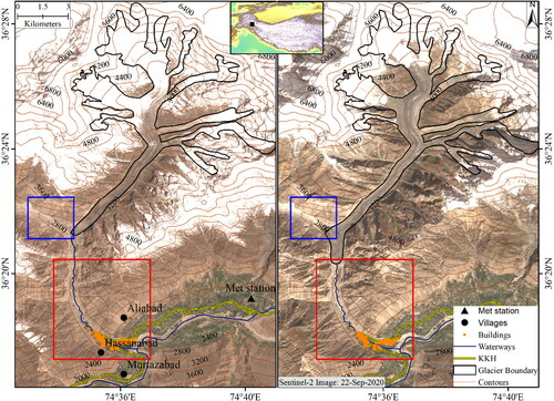
Shisper Glacier is one half of a previously much larger glacier tongue, separated into two after 1950, with the western branch referred to as Muchuhar Glacier (the lower tongye after Shisper and Muchuhar merge is refer to as Hassanabad Glacier). The glacier has been subject to repeated surges, the most recent in 1973 and 2000/2001 (Bhambri et al. 2020). Two recent studies (Bhambri et al. 2020; Rashid et al. 2020) have investigated the recent surge. Although they investigated the same event with similar data, they reached contending conclusions. Bhambri et al. (2020) provided an analysis of velocities dating back to the 1990s. They found considerable seasonal variation in surface velocities in the quiescent phase that is greatly surpassed by an increase during the recent surge in 2018 where peak velocities reached 18 m d⁻¹ in June. They also found that the lake grew to a volume of ∼ 16 × 106 m³ in May 2019, which could result in discharge of up to 400 m³ s⁻¹ and found little evidence for inundated areas but discernible channel migration due to the flood. They noted that the lake volume and discharge values should all be treated with caution due to the limited number of available data points and the empirical relations employed. Rashid et al. (2020) only investigated the recent surge with contrasting findings compared to Bhambri et al. (2020). Their peak surge velocities in 2018 stand at 48 m d⁻¹ in October, at a time when Bhambri et al. (2020) only noted velocities below 5 m d⁻¹ which might be attributed to the use of satellite data with clouds and snow (Bhambri et al. 2020). Based on similar estimates of lake volume but an empirical equation for moraine dam breaks they further estimated potential flood volumes between 5000 and 6000 m³ s⁻¹. Neither of the two studies looked into downstream impacts in much further detail.

To clarify these large discrepancies and discuss the actual downstream impacts of such a flood in more detail, we revisit this surge. Based on a more detailed investigation of downstream impacts, we aim to clarify the actual potential hazard posed by glacier surges in the region. To this end, this study aims to elucidate the following: (a) estimate the temporal variations in the glacier surge and lake reformation between 2018 and 2020, (b) comparative estimation and confirmation of ice velocity using passive and active remote sensing datasets including Sentinel-1 and Sentinel-2, (c) conduct a lake outburst model with multiple scenarios and discuss the downstream impacts, and (d) evaluate the downstream socio-economic impacts based on household questionnaires, damage analysis, and propose potential nature-based solutions to reduce the flood risk.

Datasets

We used Landsat 8 OLI images between 2016 and 2020 to understand the glacier dynamics during the quiescent and active phase. We used this dataset to assess the terminus advance and lake reformation (Table S1). Besides, Advance Space borne Thermal Emission and Reflection Radiometer (ASTER) stereo-pairs data acquired from https://earthdata.usgs.gov were used to generate digital elevation models (DEM) using the open-source Ames Stereo Pipeline (ASP) (Shean et al. 2016; Brun et al. 2017). We used Sentinel-2 L1C images between April 2018 and July 2019 to derive the horizontal flow velocity of the Shisper glacier. To verify the horizontal velocity derived from Sentinel-2 images (optical), Sentinel-1A images (SAR) between April 2018 and April 2019 were also acquired. In addition, a household socio-economic survey in the Hassanabad Valley was conducted to identify potentially vulnerable population.

Table 1. Population vulnerable to Shisper glacier outburst flood by gender and age.

Age group	Male	Percentage	Female	Percentage	Total
Households > 65 years of age	31	7.9	38	9.7	69
Household between 45 and 65 years age	69	17.6	62	15.9	131
Household between 30 and 45 years age	87	22.1	80	20.5	167
Household between 15 and 30 years age	126	32.1	120	30.7	246
Household <15 years of age	80	20.4	91	23.3	171
Total	393	100	391	100	784

Methodology

Remote sensing data

The glacier terminus advance and lake formation were mapped using Landsat 8 OLI data by manual digitization. The time-series changes in the glacier area and terminus advance during the surging of Shisper glacier and the ice-dammed glacial lake were mapped and analyzed. Besides, the phase-correlation function of the COSI-Corr software was implemented to derive the east and north glacier displacements from Sentinel-2 images (Leprince et al. 2007). After multiple experiments, we found setting an initial search window size of 64 × 64 pixels, a final search window size of 16 × 16 pixels, a search step of 2 pixels, and a correlation threshold of 0.9 can obtain good displacement fields. Only the NIR band (band 8) of Sentinel-2 images was used for the phase-correlation since it has the highest resolution of 10 m and the widest bandwidth. Systematic bias caused by the orbit change was removed by fitting a quadratic polynomial surface trend based on the observations over stable regions (Ding et al. 2016) (Figure S3). The outliers in the displacement maps resulted from cloud cover, sharp surface change, image shadow, or the lack of texture contrast were manually masked out by referring to the signal-noise-ratio map. Non-local mean filtering was performed to reduce the residual noises. Finally, the average horizontal flow velocity fields were obtained by combining the east and north displacement fields and dividing the results with image pair intervals. The intensity-tracking function of the GAMMA software was implemented to derive the glacier displacements in SAR azimuth direction and slant range direction from Sentinel-1 images (Strozzi et al. 2002). To reduce the topographic effects, the 1-arc second SRTM DEM was used to assist the SAR intensity tracking (Li et al. 2014). The size of the matching window (96 pixels in slant range direction ×72 pixels in azimuth direction) and the threshold of cross-correlation (0.3) was determined carefully to balance the result details and the number of effective observations. In general, a smaller matching window and higher cross-correlation threshold would bring in finer displacements; however, the proportion of effective observation would be lower. Similarly, non-local mean filtering was performed to suppress the noise in the displacement fields. The final average horizontal flow velocity fields were obtained by synthesizing the azimuth and slant range displacement fields and dividing the results with image pair intervals. The uncertainty of the horizontal glacier flow velocity was evaluated by the standard deviation of the observations over stable regions, where the flow velocity should be zero. The Sentinel-1 and Sentinel-2 images used in this study are listed in supplementary Table S2.

The void-filled Shuttle Radar Topography Mission (SRTM) DEM with 30 m resolution was used as a seed DEM for generating four ASTER DEMs. The latter were then coregistered horizontally and vertically to the SRTM DEM (e.g., Berthier and Brun 2019). The ASTER DEMs were also validated using differential Global Positioning System (dGPS). In this study, we used same dGPS as in Muhammad and Tian (2016, Muhammad and Tian 2020). The dGPS data and off-glacier elevation difference of ASTER DEMs are shown in Figure S5. All pixels with absolute elevation differences larger than 150 m were discarded in the analysis. Due to the haze and clouds in the ASTER images, there were some data gaps in the elevation difference maps. The volume of transported ice mass was calculated after interpolating the data gaps using natural neighbour method.

GLOF simulations

We employ the BASEMENT model (BASEMENT, 2020) to simulate two observed GLOFs from the lake formed at the terminus as well as two simulations of potentially bigger events. As in a similar recent case in the region on Khurdopin Glacier (Steiner et al. 2018), the lake at Shisper drained subglacially and water exited at the glacier terminus. No information is available about the formation of the subglacial drainage network and we hence only model the flood from the terminus of the glacier to the confluence of the local Hassanabad River into the Hunza River, which covers a distance of approximately 7 km, from 2460 m a.s.l. to 2000 m a.s.l. (slope ∼5° at the glacier terminus and ∼3° at the confluence). We use an 8 m DEM which is available from the glacier snout to the entry point (Shean 2017). Unfortunately no locally measured river cross profiles are available to verify the DEM. We therefore only correct obvious artifacts in the DEM, which were only present at one location at the terminus of the glacier. Using the lake area just before and after the drainage of the lake, we derive the volume of the lake using the 30 m SRTM DEM, which was acquired when no lake was present.We use this volume to calculate a peak discharge following Huggel et al. (2004) and (Walder and Costa 1996). (1) $$Q_{\mathit{max}}=\mathrm{}46\mathrm{}{\left(\frac{V}{{10}^6}\right)}^{0.66}$$(1) where Q_max is peak discharge in m³ s⁻¹ and V is the drainage volume in m³. The equation is specifically suited for tunnel drainage through the ice, which is what has happened at Shisper and previously at Khurdopin Glacier (Steiner et al. 2018). A more detailed discussion of the process is provided in (Bazai et al. 2021).

Measurements of peak discharge during the two outburst events in 2019 and 2020 (142 and 85 m³ s⁻¹) as well as the observation that the drainage lasted approximately 2 to 3 days enable us to recreate an input hydrograph for both events that drains the complete observed volume change. Measurements of peak discharge were conducted by the Pakistan Meteorological Department (PMD) at the main bridge in Hassanabad (PMD 2021). The basic discharge, based on ground observations is 20 m³ s⁻¹, which was also used to wet the model domain before the discharge from the lake breach was added. Beyond the standard assumptions to solve the numerical algorithms in BASEMENT, we chose a Manning-Strickler coefficient of 33 m³ s⁻¹ for the river bed and 30 m³ s⁻¹ for the surrounding area (Vanzo et al. 2021). We carefully delineated the river bed using a Sentinel-2 image from the 20th of June 2019. In the narrower sections, including the lower areas where infrastructure is affected, the river channel is between 50 and 80 m wide, in some wider parts upstream it reaches up to 200 m (Figure 1).

Socioeconomic survey

A household owning any type of property, i.e., a house, animal shelter, a business, agricultural, and nonagricultural land in the flood catchment area were considered. A total of 136 households were identified, of which 115 were found at the time of the survey. The total population covered is 784 persons (Male = 393, Female = 391). Data has been collected using mixed-method approach. Quantitative data was collected using a structured household survey questionnaire comprising of household-level socioeconomic indicators and associated vulnerabilities due to GLOFs over the last four years, i.e., as of 2017. For the household survey, household heads were interviewed. Besides, qualitative data was collected through 4 focus group discussions (FGDs).

Results and discussion

Terminus advance of shisper glacier

Shisper is a 16.5 km long surge-type glacier covering an area of 25.84 km² as per 2016 images which remained unchanged till early May 2018. The glacier terminus advance started in June 2018 and continued until July 2019. Between April and December 2018, the terminus of Shisper Glacier had advanced by 0.44 km increasing the glacier area by 0.45 km² (∼2%, Table S3). During the periods December 2018 to January 2019, January to February 2019, March to April 2019, and April to July 2019, the glacier terminus advanced by 0.74 ± 0.03 km, . 0.18 ± 0.002km, 0.09 ± 0.005 km, and 0.27 ± 0.004 km, respectively. After July 2019, the advance was very slow and the terminus became almost stationary from November 2019 until the observed time of October 2020. This suggests that the surge has two repeat peak cycles in 2018 and 2019. The glacier terminus advance and increase in the area during the whole surge period was 1.79 km and 1.40 km² (Table S3). The present terminus advance was modest compared to past advances of 9.3 km and 9.8 km for the 1892-93 and 1903surges, respectively (Goudie et al. 1984, Hewitt 2014).

Formation and breaching of ice-dammed glacial lake

The surging mass of the Shisper Glacier blocked the meltwater channel of the adjacent Muchuhar Glacier, forming an ice-dammed lake from mid-November 2018 (Figure 2). The glacier terminus completely blocked the valley ∼1.5 km Hassanabad River. The lake occupied an area of 0.042 km² during November 2018. We also found an abrupt increase in maximum temperature of the nearby meteorological station at Ali Abad, Hunza during April and June 2018 when the surging ice was reported to accelerate and reached its peak (Bhambri et al. 2020). The lake level gradually increased between November 2018 and 20 June 2019 to form an ice-dammed lake with an area of 0.31 km² (Table S3). Two days before the outburst on June 20, 2019, the lake reached an area of 0.35 km². The GLOF on June 22, 2019, partially damaged the Karakoram Highway and caused minor infrastructure damage downstream. In July 2019, the lake shrinked to an area of 0.2 km², and in August the lake further reduced to 0.03 km². In September 2019, lake water drained almost completely. In October 2019, a lake again started to form and covered an area of 0.04 km². In November 2019, the lake area increased abruptly up to 0.22 km². An adjacent ice-dammed lake was formed between the Shisper Glacier margin and valley wall (supplementary Figure S1). The lake slowly drained out as indicated by a reduction in lake size by 0.008 km² between March and April 2020. This event was not reported in local media as the locals may have not noticed the insignificant rise in flow. In May 2020, two ice-dammed lakes merged to form a single ice-dammed glacial lake. The size of the merged lake was 0.25 km² a day before the breach (Table S3). On 29 May 2020, the lake breached causing an inundation of 0.6 km² and partially damaged a 700 m stretch of the Karakoram Highway (supplementary Figure S2).

Figure 2. Snout change and lake formation and change from 2018 to 2020 (a). The blue and black lines are the terminus extent in the quiescent and post-surge, respectively. The minimum and maximum temperature data at Hunza meteorological station is also shown (b).

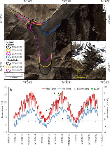
The 2018-2019 active surging behaviour of Shisper Glacier, dynamic features of the ice-dammed lake and the past two major GLOF events in June 2019 and May 2020 indicate that the lake might expand its size again and there is a chance of another GLOF in the future. The greater risk is in summer months between April and September. Currently, field-based lake monitoring is almost impossible as the glacier surge mass has blocked the access to the valley. Therefore, regular spaceborne remote sensing monitoring of the lake is imperative until the surged ice which blocks the Muchuhar stream completely melts away.

Flow velocity change of shisper glacier

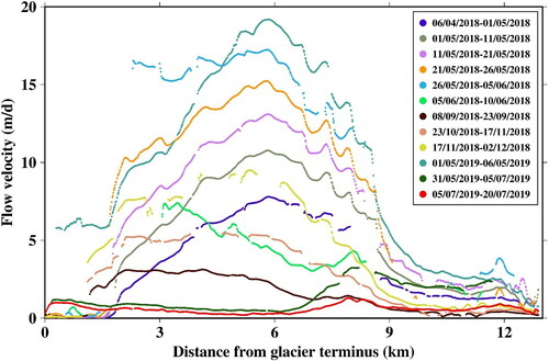
The time series of horizontal flow velocity derived from Sentinel-2 imagery indicated the Shisper Glacier surged two times between April 2018 and July 2019. As shown in Figures 3 and 4, the tongue of Shisper Glacier accelerated from early April 2018 (7.8 m/d) to early June 2018 (17.2 m/d) and then decelerated from early June to late September 2018 (3.2 m/d). However, it accelerated again from late September 2018 to early May 2019 (19.2 m/d) and then decelerated from early May to late July 2019 (1.4 m/d). The acceleration mainly occurred at the trunk of the Shisper Glacier, which is consistent with distribution of surface elevation change caused by the surge activity (Figures 3 and 4). During the surge phase, the flow velocity generally increased from the upper trunk to the mid-lower trunk, and then decreased towards the terminus. However, during period 26 May to 5 June 2018, the velocity did not decrease at the mid-lower trunk; the velocity of the middle trunk and lower trunk was high and uniform (∼16 m/d), indicating a large volume of mass was discharged during this short period. At the upper trunk (10 ∼ 13 km from the terminus), the flow velocity actually increased downstream very slowly, even during the most active periods (26/5/2018 to 5/62018, 1/5/2019 to 6/5/2019). However, at the confluence of the trunk with the lowest tributary (i.e., the valley mouth), the flow velocity increased sharply, because the bed becomes narrow and steep there. The highest horizontal flow velocity (19.2 ± 0.16 m/d) occurred 5.8 km from the terminus during the period 1 May to 6 May 2019 (Figures 3 and 4). At the same place, the horizontal flow velocity during the period 5 July to 20 July 2019 was only 0.30 ± 0.16 m/d. The temporal change in flow velocity is consistent with that in terminus advancing speed. As mentioned above, the terminus advance was very slow after July 2019. Note that during the period 5 July to 20 July, the flow velocity at the terminus was higher than that at the mid-lower trunk, where the flow velocity reached the peak during the surge phases (see Figure 3). After the second surge, a large volume of mass (302.8 × 10⁶ m³) was transferred from the upper reaches to the glacier snout. Driven by the gravity effects, the transferred mass did not stop advancing immediately, even though there was no compressing stress from upper reaches. It kept flowing downslope until the resisting force equalled the driving force.

Figure 3. Time series of the horizontal flow velocity of the Shisper Glacier derived from optical imagery (Sentinel-2). Background: shaded SRTM DEM; black curve: glacier outline; dashed line in panel l: location of the profile shown in Figure 4.

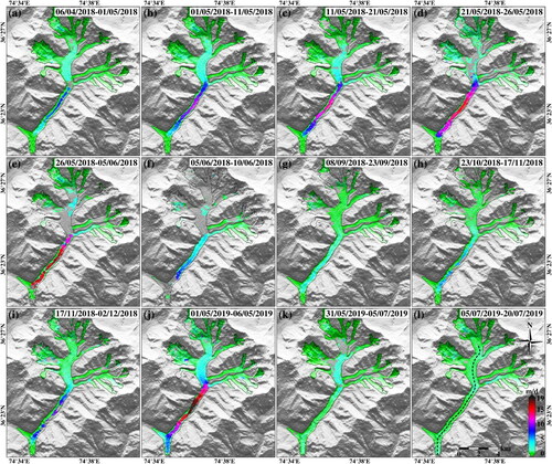
Figure 4. Spatial variation in the horizontal flow velocity along the profile shown in Fig. 3l.

Bhambri et al. (2020) derived a time series of flow velocity from Sentinel-2 images. Their results also indicated the Shisper Glacier accelerated two times during 2018 to 2019. They found the peak of the flow velocity (∼18.0 ± 0.5 m/d) at the mid-lower trunk during period 21 April to 6 May 2019. The slight difference between our peak velocity (19.2 ± 0.16 m/d) and theirs may be due to the slight difference of observation periods. As shown in Figures 3 and 4, the flow velocity in the period 1 May to 6 May 2019 is higher than that during the period 21 April to 1 May 2019. In general, both the temporal and spatial change pattern of our optical flow velocity during 2018 to 2019 are consistent with that derived by Bhambri et al. (2020); however, our flow velocity fields have higher coverage and richer details, especially in the upper trunk. In the study of Rashid et al. (2020), the maximum flow velocity of the Shisper Glacier was much larger (over 45 m/d in late 2018 and early 2019). Their results were derived from Landsat-8 OLI images, which has a coarser spatial resolution and sparser temporal distribution than Sentinel-2 images. Moreover, many outliers induced by the cloud and fresh snow (lead to the lack of texture contrast) were preserved in their results. This explains the large difference in results.

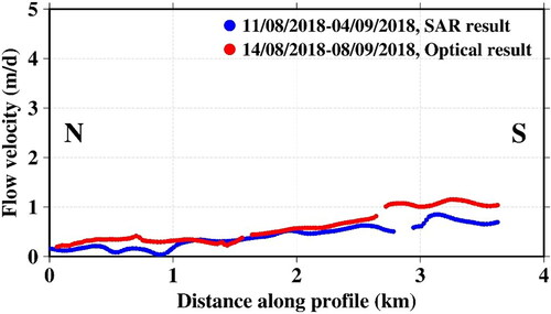
Due to the slant-range imaging way, the glacier tongue located in the deep valley was hardly illuminated by the Sentinel-1 radar. Therefore, over the glacier tongue, no effective displacements could be obtained from the Sentinel-1 images (Figure 5). Nevertheless, the variation pattern of displacements obtained over the broad upper reaches is consistent with that derived from Sentinel-2 imagery. The time series of Sentinel-1 flow velocity (Figure 5) shows the upper reaches of the Shisper Glacier accelerated from early April to late May 2018, and decelerated from early June to early September 2018, and then accelerated again at early April 2019. Sentinel-1 and Sentinel-2 horizontal flow velocities profile closely matches with some uncertainty (Figure 6).

Figure 5. Time series of the horizontal flow velocity of the Shisper Glacier derived from SAR imagery (Sentinel-1). Background: shaded SRTM DEM; black curve: glacier outline; dashed line in subfigure g: location of the profile shown in Figure 6.

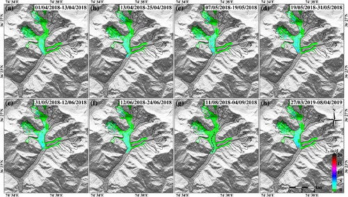
Figure 6. The optical- and SAR-based horizontal flow velocities along the profile shown in Figure 5g.

In general, both Sentinel-2 and Sentinel-1 flow velocity results show that the Shisper Glacier accelerated in winter/spring and decelerated in summer, which is a typical feature of hydrologically-controlled glacier surge (Kamb 1987; Round et al., 2017). It is likely that the basal water pressure increased in winter/spring and promoted the glacier acceleration; however, as the collision and compression of ice bodies intensified during the surge phase, part of the basal meltwater drained in early summer and the glacier decelerated correspondingly. Hence, the Shisper Glacier may surge again in the coming decades. To some extent, no matter how much mass the Shisper Glacier accumulates at its upper reaches, it will surge as long as its basal water pressure is high enough.

Elevation changes of shisper glacier

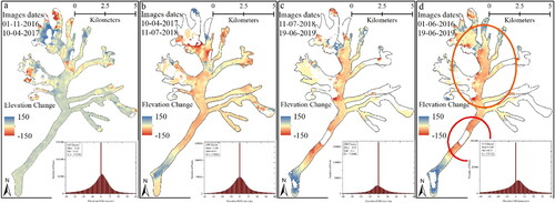
Four DEMs acquired on 1 November 2016, 10 April 2017, 11 July 2018, 19 June 2019, respectively were compared with each other to estimate the ice transfer from the accumulation to ablation zones (Figure 7). The difference between the first two DEMs indicated that no surge occurred before April 2017. We used the DEM from April 2017 as pre-surge DEM because no other ASTER stereo-pairs are available until the start of the surge. The DEM differencing indicate that glacier ice surged from the upper zones >10 km above the terminus. The elevation changes due to the surge are more prominent in the lowest part where the ice accumulated below the lower-middle narrow valley causing internal deformation and extensive crevasses. The surge indicates a complex triggering mechanism as the mean surface lowering in the upper part is nearly −9 m whereas the lower middle part indicates approximately −60 m between 2017 and 2019 (encircled in Figure 7(d)). These results are also confirmed by the horizontal flow velocity where a comparatively slow and fast glacier movement of < 5 m and up to ∼19 m/day is observed in the upper and lower glacier part, respectively (Figure 3j-k). The surged ice accumulated in the ∼3 km above the post-surge terminus position with an average elevation increase of approximately +94 m between April 2017 and June 2019. The difference of the DEMs indicated an ice mass transport of 96.5 × 10⁶ m³ between April 2017 and July 2018 which increased to 206.3 × 10⁶ m³ between July 2018 and June 2019 (Figure 7). Bhambri et al. (2020) estimated a net mass gain of 251 ± 67 × 106 m³ between October 2017 and June 2019. The volume of the surge and mass relocation of the Shisper Glacier is quite sizeable, more than twice the Horcones Inferior Glacier surge (Mount Aconcagua, Central Andes) (Pitte et al., 2016) and ∼10% more than the Khurdopin Glacier (Steiner et al. 2018). In addition, the Shisper Glacier surged ice is approximately 60% and 67% more than that of the collapsed ice (68 ± 2 × 10⁶ m³ and 83 ± 2 × 10⁶ m³) of twin Aru Glaciers (Kääb et al. 2018), and approximately 37% more than that of the disintegrated ice (130 × 10⁶ m³) of the Kolka Glacier (Evans et al. 2009).

Figure 7. Surface elevation changes of Shisper Glacier between 2016 and 2019. The ice surged from the zones encircled in (d). The surged ice accumulated near the terminus as visible in blue colour whereas the white spots are missing data due to clouds.

Outburst flood simulations

We obtained the drained volume during the two events in 2019 and 2020 by comparing the lake volume before and after the drainage resulting in approximately 9.7 and 4.8 million m³ drained respectively. Using the calculated peak discharge (equation 1(1) $$Q_{\mathit{max}}=\mathrm{}46\mathrm{}{\left(\frac{V}{{10}^6}\right)}^{0.66}$$(1) ) we were able to distribute the total discharge over the time where the high flow was observed downstream, i.e., 48 hours (Figure 8). The lake drained subglacially, i.e., meltwater after it accumulated and likely warmed up continuously excavated a tunnel through the ice at the lake and then exited the snout 2 km further down, with an elevation drop of approximately 150 m (Figure 9). While moraine dam breaks are expected to have a hydrograph that peaks rapidly, tunnel excavation takes time and the hydrograph is expected to slowly rise, culminate at a sudden peak as it reaches a critical diameter and the quickly drain completely (Walder and Costa 1996). This matches observations from the field, where from 22^nd to 23^rd of June 2019 a steady increase was observed over 24 h, discharged peaked at 142 m³ s⁻¹ at night the 24^th June and then gradually decreased to the previous rate. However, the exact start of lake drainage is not known and neither is the drainage mechanism understood. We, therefore, run a number of scenarios to evaluate downstream effects. The modelled peak discharge (206.1 and 129.5 m³ s⁻¹) is well above the measured discharge in the village at the bridge (located where the KKH crosses the river, Figure 10) of 142 and 85 . This can be explained by the expected attenuation of the flood peak between the glacier snout and the measurement location as well as the general uncertainty of the measurement during peak flow and the relatively wide confidence interval of Equation (1)(1) $$Q_{\mathit{max}}=\mathrm{}46\mathrm{}{\left(\frac{V}{{10}^6}\right)}^{0.66}$$(1) (Walder and Costa 1996) . As an extreme scenario we additionally evaluated a hypothetical lake drainage, where 27.6 million m³ would be drained assuming that the lake could grow to approximately twice the observed size of 348000 m² in 2019. This results in a peak discharge of 410 m³ s⁻¹ (referred to as “hyp” in Figure 8), which corresponds to the value used in Bhambri et al. 2020.

Figure 8. (a) The glacier terminus in 2019 when the surge was still active. The blue arrow denotes the location of the lake, the orange dashed line shows the trim line of the old tongue of Muchuhar Glacier when both branches of the old Hassanabad Glacier were still connected (pre 1950). (b) Shows the lake in 2019, at the location where eventually the ice tunnel would open. (c) A panorama view taken from East to West just below the terminus at the approximate maximum extent, where the GLOF would exit the glacier tongue.

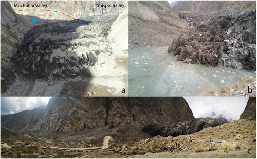
Figure 9. Input hydrographs for the observed GLOFs in 2019 and 2020 as well as the hypothetical example (hyp). 2019* is the same drained volume as in the normal scenario, only with a later peak. The two triangles show the empirical expected peak discharge following Huggel et al. (2004) for the two observed events.

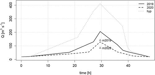
Figure 10. Outburst flood simulations. The green background shows vegetation and agricultural land based on a Landsat image from the 22nd of July 2019 (NDVI > 0.1). The background is a Sentinel-2 image from the 20th of July 2019. Note that the simulation stops at the confluence with the Hunza River and the water level from the main arm is derived from the NDVI rather than the simulation. Contour lines are placed every 100 m. (a) Overview over the complete model domain. The black square shows the details shown in panels b-e. (b) Water depth during the simulation in 2019 at peak flow. The white arrows pointing away from the bridge towards houses show the view visualized in Figure 11. The small red arrow show a diversion canal for irrigation. The part of the highway marked in red was damaged during the event in 2019 (Figure 10c). (c) Shear stress during the event in 2019 at peak flow. (d/e) Flow velocities during the 2019 and hyp scenario respectively.

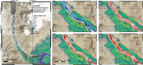
The discharge peak reaches the settlement approximately 1.5 h after it exits the lake. In Figure 10a, the simulation results for 2019 are shown for the complete domain at the moment that the flood peak reached the bridge in Hassanabad. As observed during the event, the water stayed largely within the incised channel, causing flooding of agricultural land on the left channel bank before the settlement and again after the bridge. In the simulation water reaches one house that is located close to the river channel, on the right river bank looking downstream from the bridge as well as one on the opposite bank upstream (Figure 11a). This corresponds with the observation made in the field, where the downstream house was indeed reached by high water (Figure 11b), while the house upstream was just not reached due to the construction of a new embankment (Figure 11a). Additionally some of the orchards along the river bank are inundated at various locations, especially before and after an intake to an irrigation channel (Figure 10b), in line with observations. Most of the damage has been reported on trees, agricultural land and irrigation channels close to the main channel.

Figure 11. Photographs of the river around peak flow upstream (a) and downstream (b) of the bridge crossing the river in Figure 10. Damage caused to the road downstream of the bridge (c).

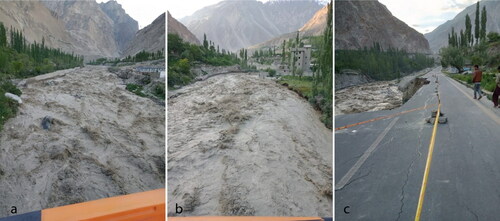
Increasing the discharge drastically as in the hyp scenario, does not cause significant additional area to be inundated. However, the extreme discharge volumes cause indirect damage via erosion of embankments, in the extreme case causing the collapse of adjacent infrastructures such as the Highway which is the main road in the region and the only direct connection between China and Pakistan (Figure 11). As there is little space for the discharge to dissipate, flow velocities increase strongly. Modelled velocities around the bridge and further downstream were around 4 to 6 m s⁻¹ for the scenario in 2020, between 5 and 7 m s⁻¹ in 2019 and increasing to 10 m s⁻¹ in the hyp scenario. Shear stress τ was ∼300 N m⁻² in 2019 and reached up to ∼600 N m⁻² also close to embankments.

There are a number of uncertainties in modelling lake outbursts in an environment with little available observation data. First, GLOF simulations are sensitive to DEM quality (Watson et al., 2015). The model does not include recently erected embankments (Figure 10a/b) and is only based on the DEM. Further improvements could be made with accurate cross-section measurements from the field. However, the fact that modelled and observed discharge levels during the outburst in 2019 agree well support the potential of recently available and easily accessible high resolution DEMs, like used in this case (Shean 2017).

Deriving lake volumes from lake areas introduces additional uncertainty. Our volume estimates (2.17 10⁷ m³ and 1.71 10⁷ m³) fall well within the uncertainty bar of the estimated volumes at Shisper from Bhambri et al. (2020). However, as Bhambri et al. 2020 and Rashid et al. 2020 note and the large difference in estimated discharge volume between ∼400 m³ s⁻¹ and ∼5000 m³ s⁻¹ visualize, coming to an appropriate estimate for peak discharge, that is defining for potential downstream hazards remains extremely difficult. We can readily rule out the extreme estimate from Rashid et al. 2020. It is based on an empirical equation derived for moraine dam breaches, where all accumulated water discharges rapidly (within ∼1 hour) in an extreme flood wave. Such a discharge would be more than 3 times the peak discharge during summer at Danyore, approximately 70 km downstream near Gilgit where the entire Hunza catchment is captured (∼1500 m³ s⁻¹). While events of such dimension can happen in theory, it would be very unlikely for an ice-dammed case (where more time is needed to carve and enlarge a tunnel through the ice) and has not been confidently observed previously in the region. Historic observations of the Kyagar GLOF were in that order of magnitude, but the present lake which has a much larger volume than the Shisper Lake would create a much smaller flood wave of 1500 m³ s⁻¹. Other historic accounts report similar extreme values up to 7000 m³ s⁻¹ but are all based on very rough estimates of total discharge times (Hewitt 1982; Iturrizaga 2005; Hewitt and Liu 2010) Our field observations of relatively moderate peak discharge of just above 100 m³ s⁻¹ and high flows spanning up to 2 full days, suggest that such extreme assumptions are misplaced. While flood peak attenuation after GLOFs can be considerable in the HKH (Schwanghart et al. 2016, Maurer et al. 2020), it is unlikely to be an order of magnitude over this relatively short distance of 4.5 km. Future studies should investigate in more detail how rapid attenuation happens in such small streams with heavy sediment load to better understand the threat of GLOFs to downstream communities. Nevertheless, the relatively low peak flows investigated here (∼100 to 400 m³ s⁻¹) are capable of causing considerable erosive damage. Increasing the flood further to the higher estimate from Bhambri et al. (2020) generally does not increase inundation area significantly but flow velocity and erosive potential in the main channel. At these forces, boulders with ∼1 m diameter are easily moved (Costa 1983, Shields 1936). This reflects the potential of GLOFs to move a large amount of sediments within a short period of time. As further sediment supply from upstream is cut off due to the blockage caused by the surge (assuming that most of the subglacially transported material is suspended load) causes the river channel downstream to incise ever deeper, causing further instabilities in future. As the lake is likely going to form in subsequent years repeatedly, this could cause serious destabilization of the complete Hassanabad deposit. A countermeasure for this development would be the removal of embankments upstream to give the water more space to decrease river flow velocities and attenuate the peak discharge. Further analysis would be needed to determine erosion rates. Such estimates would also be of interest for the fraction of total sediment load in the Hunza River being sourced from such extreme events. Simulations including sediment transport and a more realistic dam break and tunnel formation scenario could further elucidate important processes, but introduce further uncertainties that are difficult to constrain.

Socio-economic impacts

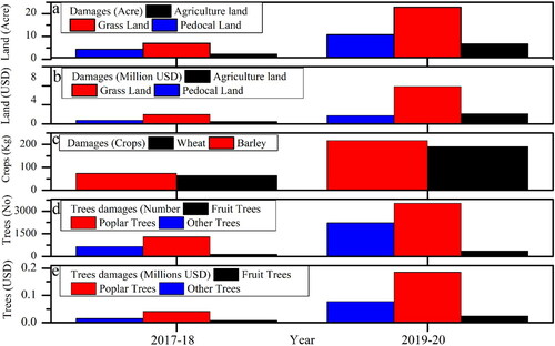
Mountain communities are highly concerned about the consequences of huge GLOF during ever-increasing temperatures during summers. In the Karakoram Mountains, floods mostly occur in early spring until late summer where smallholder farmers’ agricultural activities remain at the peak in the same season. To evaluate the impact of GLOFs of Shisper Glacier, a total of 115 households were surveyed for the detailed socio-economic damages assessment (Table 1). The average household size is equivalent to the national average of ∼6.8 (Pakistan Bureau of Statistics (PBS) Pakistan Bureau of Statistics (PBS)) 2013). The average age of the population is ∼33 years, with most people between 15 and 30 years followed by children below 15 years and adults between 30 and 45 years. About 13.7% and 5.8% of the population have graduation and master qualification, respectively. The GLOFs in 2019-20 caused catastrophic damages to all three land categories. Each of the 115 GLOF affected households sustained an economic loss of 35,000 USD during the last four years, approximately 4 million USD as a whole. The grassland owner communities and smallholder farmers bear huge losses almost every summer. The 2019-20 GLOFs damaged a total of 22.82 Acre of grassland, 10.02 Acre of Pedocal land, and 6.77 Acre of agricultural land. On average, each of the 115 GLOF-affected households lost approximately 0.47 Acre land. A total of 8217 fruit and non-fruit trees were destroyed between 2017 and 2020, from both general high melt water discharge and GLOFs. Shisper stream remains flooded almost every summer and badly damages vulnerable infrastructure mainly including 3 major irrigation channels serving as the lifeline of Murtazaabad, Hassanabad, and Aliabad. The 2020 GLOF damaged drinking water pipeline and other infrastructure in these villages. Shisper stream remain flooded almost every summer and badly damages vulnerable infrastructure mainly including 3 major irrigation channels serving as the lifeline of three major villages, i.e., Murtazaabad, Hassanabad, and Aliabad. During peak floods, the community rehabilitate main water channels requiring huge human efforts and life-threatening situation during rehabilitation workIn 2019-2020, a total of 6126 trees constituting 369 fruit trees, 3525 Poplar trees, and 2232 other trees were damaged as a result of the GLOFs having an economic value of 0.29 million USD. The land and trees damages and associated economic losses are shown in Figure 12. During peak floods in summer, the community rehabilitate the main water channels requiring large human efforts and resulting in potentially life-threatening situations. They are being faced with the challenge of not being able to counter the repeat GLOF occurrence. In such a situation, a flood early warning system may help to prevent human lives and damages to scarce properties of poor stallholders. To save the lives, assets, and properties of vulnerable communities, we recommend that: i) End-to-end ‘Gabion Walls’ are constructed, ii) Construction of barriers to reduce the flood flow, iii) Allocation of development funds for routine rehabilitation of critical water infrastructure, and iii) Permanent resettlement of vulnerable people.

Figure 12. Socio-economic damages and losses downstream Shisper Glacier between 2017 and 2020.

Conclusion

The repeated Shisper Glacier surge possess a potential risk to downstream people and livelihoods. The glacier surge is not directly hazardous to the distant (> 5 km) downstream population. The peak glacier velocity was 19.2 ± 0.16 m/day in May 2018 and May 2019 which continued to flow with normal velocity after September 2019. However, the surged ice retained Muchuhar Glacier meltwater in an ice-dammed lake creating a continuous threat until the surged ice completely melts away. The ice-dammed lake started to form in November 2018 and outburst on June 22, 2019, for the first time. An early winter (January 2020) lake outburst occurred, reported by locals, was not captured through remote sensing because of the frozen lake surface, followed by a third outburst in April 2020. Simulations of the June 2019 event with a modelled peak discharge of 206.1 m³ s⁻¹ and 129.5 m³ s⁻¹ in April 2020 agree well with observed discharge and inundated land. Water flow velocities during the June 2019 event reached up to 7 m s⁻¹ close to the settlement and would increase up to 10 m s⁻¹ in a hypothetical case where the lake would be twice as large. Even during very high flows, relatively little land is inundated and most damages are along the embankments and the poplar trees planted along the river. Our results suggest that the biggest hazard of the lake outburst lies in its erosion potential, resulting in damages to infrastructure immediately next to the river as well as a potentially large output of sediments to the downstream Hunza River. The outburst destroyed a powerhouse and partially damaged ∼700 m of the Karakoram Highway. The downstream 115 households faced economic losses of 4 million USD between 2017 and 2020. The losses are mainly due to damages of agriculture land, crops, and trees. Each household faced approximately 35,000 USD of losses between 2017 and 2020. To reduce the future damages in the valley, installation of gabion walls along the Hassanabad stream to overcome erosion, building barriers to reduce the flood water flow, and installation of an early warning system are recommended.

Acknowledgement

The views and interpretations in this publication are those of the authors. They are not necessarily attributable to ICIMOD and do not imply the expression of any opinion by ICIMOD concerning the legal status of any country, territory, city or area of its authority, or concerning the delimitation of its frontiers or boundaries, or the endorsement of any product. This work was supported by ICIMOD’s Cryosphere Initiative funded by Norway and by core funds of ICIMOD contributed by the governments of Afghanistan, Australia, Austria, Bangladesh, Bhutan, China, India, Myanmar, Nepal, Norway, Pakistan, Sweden, and Switzerland. The views and interpretations in this publication are those of the authors and are not necessarily attributable to ICIMOD. We thank a group of 10 master students and a faculty member of the Hunza campus of Karakoram International University (KIU) for carrying out the collection of household-level data. EB acknowledges support from the French Space Agency (CNES).

Disclosure statement

No potential conflict of interest was reported by the authors.

Data availability statement

The data of this study are available from the corresponding author upon reasonable request.

Additional information

Funding

This research has been supported by the International Centre for Integrated Mountain Development (ICIMOD; grant no. 3-939-241-0-P).

References

- BASEMENT. 2020. BASEMENT – Basic Simulation Environment for Computation of Environmental Flow and Natural Hazard Simulation. Version 3.1.1 © ETH Zurich, VAW, 2020.
- Bazai NA, Cui P, Carling PA, Wang H, Hassan J, Liu D, Zhang G, Jin W. 2021. Increasing glacial lake outburst flood hazard in response to surge glaciers in the Karakoram. Earth-Sci Rev. 212:103432.
- Berthier E, Brun F. 2019. Karakoram geodetic glacier mass balances between 2008 and 2016: persistence of the anomaly and influence of a large rock avalanche on Siachen Glacier. J Glaciol. 65(251):494–507.
- Bhambri R, Hewitt K, Kawishwar P, Pratap B. 2017. Surge-type and surge-modified glaciers in the Karakoram. Sci Rep. 7(1):15391.
- Bhambri R, Watson CS, Hewitt K, Haritashya UK, Kargel JS, Pratap Shahi A, Chand P, Kumar A, Verma A, Govil H. 2020. The hazardous 2017–2019 surge and river damming by Shispare Glacier, Karakoram. Sci Rep. 10:1–14.
- Brun F, Berthier E, Wagnon P, Kääb A, Treichler D. 2017. A spatially resolved estimate of High Mountain Asia glacier mass balances from 2000 to 2016. Nat Geosci. 10(9):668–673.
- Copland L, Sylvestre T, Bishop MP, Shroder JF, Seong YB, Owen LA, Bush A, Kamp U. 2011. Expanded and recently increased glacier surging in the Karakoram. Arctic Antarct Alp Res. 43(4):503–516.
- Costa JE. 1983. Paleohydraulic reconstruction of flash-flood peaks from boulder deposits in the Colorado front range. Geol Soc Am Bull. 94(8):986–1004.
- Ding C, Feng GC, Li ZW, Shan XJ, Du YD, Wang HQ. 2016. Spatio-Temporal error sources analysis and accuracy improvement in landsat 8 image ground displacement measurements. Remote Sens. 8(11):937.
- Evans SG, Tutubalina OV, Drobyshev VN, Chernomorets SS, McDougall S, Petrakov DA, Hungr O. 2009. Catastrophic detachment and high-velocity long-runout flow of Kolka Glacier, Caucasus Mountains, Russia in 2002. Geomorphology. 105(3-4):314–321.
- Goudie AS, Jones DKC, Brunsden D. 1984. Recent fluctuations in some glaciers of the Western Karakoram mountains, Hunza, Pakistan. In: Miller, KJ, editor. Proceedings of the Conference concerning the International Karakoram Project, Vol. 2, Cambridge University Press, pp. 411–455.
- Harrison, W.D., Osipova, G.B., Nosenko, G.A., Espizua, L., Kääb, A., Fischer, L., Huggel, C., Craw Burns, P.A., Truffer, M., Lai AW. Snow Ice-Related Hazards, Risks, Disasters 2015. p. 437–485. Glacier Surges
- Hewitt K. 1982. Natural dams and outburst floods of the Karakoram Himalaya. IAHS-AISH Publication Hydrological Aspects of Alpine and High Mountain Area (as (Proceedings of the Exeter Symposium, Juiy 1982)) (Proceedings No. 138).
- Hewitt K. 1998. Glaciers receive a surge of attention in the Karakoram Himalaya. Eos Trans Agu. 79(8):104–105.
- Hewitt K. 2007. Tributary glacier surges: An exceptional concentration at Panmah Glacier, Karakoram Himalaya. J Glaciol. 53(181):181–188.
- Hewitt K. 2014. Glaciers of the Karakoram Himalaya: Glacial environments, processes, hazards and resources. In Advances in Asian human-environmental research. Netherlands, Dordrecht: Springer.
- Hewitt K, Liu J. 2010. Ice-Dammed lakes and outburst floods, Karakoram Himalaya: historical perspectives on emerging threats. Physical Geography. 31 (6):528–551.
- Huggel C, Haeberli W, Kääb A, Bieri D, Richardson S. 2004. An assessment procedure for glacial hazards in the Swiss Alps. Can Geotech J. 41(6):1068–1083.
- Humphrey N, Raymond C. 1994. Hydrology, erosion and sediment production in a surging glacier: Variegated Glacier, Alaska, 1982–83. J Glaciol. 40(136):539–552.
- Iturrizaga L. 2005. Historical Glacier-Dammed Lakes and Outburst Floods in the Karambar Valley (Hindukush-Karakoram). GeoJournal. 63 (1-4):1–47.
- Jiskoot H. 2011. Glacier Surging. In: Singh VP, Singh P, Haritashya UK, editors. Encyclopedia of Snow, Ice and Glaciers. Encyclopedia of Earth Sciences Series. Dordrecht: Springer.
- Jiskoot H, Boyle P, Murray T. 1998. The incidence of glacier surging in Svalbard: evidence from multivariate statistics. Comput Geosci. 24(4):387–399.
- Kääb A, Leinss S, Gilbert A, Bühler Y, Gascoin S, Evans SG, Bartelt P, Berthier E, Brun F, Chao WA, et al. 2018. Massive collapse of two glaciers in western Tibet in 2016 after surge-like instability. Nature Geosci. 11(2):114–120.
- Kamb B. 1987. Glacier surge mechanism based on linked cavity configuration of the basal water conduit system. J Geophys Res. 92(B9):9083.
- Leprince S, Barbot S, Ayoub F, Avouac JP. 2007. Automatic and Precise Orthorectification, Coregistration, and Subpixel Correlation of Satellite Images, Application to Ground Deformation Measurements. IEEE Trans Geosci Remote Sensing. 45(6):1529–1558.
- Li J, Li Z, Ding X, Wang Q, Zhu J, Wang C. 2014. Investigating mountain glacier motion with the method of SAR intensitytracking: Removal of topographic effects and analysis of the dynamic patterns. Earth Sci Rev. 138:179–195.
- Longstaff TG. 1910. Glacier exploration in the Eastern Karakoram. R. Geogr. Soc. 35(6):622–653.
- Maurer JM, Schaefer JM, Russell JB, Rupper S, Wangdi N, Putnam AE, Young N. 2020. Seismic observations, numerical modeling, and geomorphic analysis of a glacier lake outburst flood in the Himalayas. Sci Adv. 6 (38):eaba3645.
- Meier MF, Post A. 1969. What are glacier surges? Can J Earth Sci. 6(4):807–817.
- Muhammad S, Tian L. 2016. Changes in the ablation zones of glaciers in the western Himalaya and the Karakoram between 1972 and 2015. Remote Sens Environ. 187:505–512.
- Muhammad S, Tian L. 2020. Mass balance and a glacier surge of Guliya ice cap in the western Kunlun Shan between 2005 and 2015. Remote Sens Environ. 244:111832.
- Pakistan Bureau of Statistics (PBS). 2013. Population by sex, sex ratio, average household size and growth rate, http://www.pbs.gov.pk/content/population-sex-sex-ratio-average-household-size-and-growth-rate.
- Pitte P, Berthier E, Masiokas MH, Cabot V, Ruiz L, Hidalgo LF, Gargantini H, Zalazar L, 2016. Geometric evolution of the Horcones Inferior Glacier (Mount Aconcagua, Central Andes) during the 2002–2006 surge. J. Geophys. Res. Earth Surf. 121, 111–127. doi:https://doi.org/10.1002/2015JF003522.
- PMD. 2021. Updated assessment on Shishper Glacier Surge and Glacier Dam Lake in Hassanabad, Hunza, Gilgit-Baltistan, https://ciic.pmd.gov.pk/wp-content/uploads/2021/02/Shishper-Glacier-Report.pdf.
- Quincey DJ, Glasser NF, Cook SJ, Luckman A, Al QET. 2015. Heterogeneity in Karakoram glacier surges. J Geophys Res Earth Surf. 120(7):1288–1300.
- Rankl M, Kienholz C, Braun M. 2014. Glacier changes in the Karakoram region mapped by multimission satellite imagery. Cryosphere. 8(3):977–989.
- Rashid I, Majeed U, Jan A, Glasser NF. 2020. The January 2018 to September 2019 surge of Shisper Glacier, Pakistan, detected from remote sensing observations. Geomorphology. 351:106957.
- RGI Consortium. 2017. Randolph glacier inventory – a dataset of global glacier outlines: Version 6.0.
- Round V, Leinss S, Huss M, Haemmig C, Hajnsek I. 2017. Surge dynamics and lake outbursts of Kyagar glacier, Karakoram. Cryosphere. 11(2):723–739.
- Round V, Leinss S, Huss M, Haemmig C, Hajnsek I. 2017. Surge dynamics and lake outbursts of Kyagar Glacier, Karakoram. The Cryosphere. 11(2):723–739.
- Schwanghart W, Worni R, Huggel C, Stoffel M, Korup O. 2016. Uncertainty in the Himalayan energy–water nexus: estimating regional exposure to glacial lake outburst floods. Environ Res Lett. 11 (7):074005.
- Sevestre H, Benn D. 2015. Climatic and geometric controls on the global distribution of surge-type glaciers: Implications for a unifying model of surging. J Glaciol. 61(228):646–662.
- Shean DE. 2017. High Mountain Asia 8-meter DEMs derived from cross-track optical imagery, version 1.
- Shean DE, Alexandrov O, Moratto ZM, Smith BE, Joughin IR, Porter C, Morin P. 2016. An automated, open-source pipeline for mass production of digital elevation models (DEMs) from very-high-resolution commercial stereo satellite imagery. ISPRS J Photogramm. 116:101–117. 2016.
- Shields A. 1936. Anwendung der Aehnlichkeitsmechanik und der Turbulenzforschung auf die Geschiebebewegung. Mitt. Preuss.-Chen Vers. F¨ur Wasserbau Schiffbau.
- Steiner JF, Kraaijenbrink PDA, Jiduc SG, Immerzeel WW. 2018. Brief communication: The Khurdopin glacier surge revisited-extreme flow velocities and formation of a dammed lake in 2017. Cryosph. 12(1):95–101.
- Strozzi T, Luckman A, Murray T, Wegmülller U, Werner CL. 2002. Glacier motion estimation using SAR offset-tracking procedures. IEEE T Geosci Remote. 40(11):2,384–2,391.
- Vanzo D, Peter S, Vonwiller L, Bürgler M, Weberndorfer M, Siviglia A, Conde D, Vetsch DF. 2021. Basement v3: A Modular Freeware for River Process Modelling over Multiple Computational Backends. Environ Modell Software. 143:105102.
- Walder JS, Costa JE. 1996. Outburst floods from glacier-dammed lakes: the effect of mode of lake drainage on flood magnitude. Earth Surf Process Landforms. 21(8):701–723.
- Watson CS, Carrivick J, Quincey D. 2015. An improved method to represent DEM uncertainty in glacial lake outburst flood propagation using stochastic simulations. Journal of Hydrology. 529(3): 1373–1389.