Spatial distribution of bedrock level peak ground acceleration in the National Capital Region of India using geographic information system

Abstract

The probabilistic seismic hazard analysis is conducted for the seismically active National Capital Region (NCR) of India, one of the most densely populated regions in the world, to quantify the peak ground acceleration (P GA) at bedrock level by considering seismogenic source characteristics, smoothened grid seismic zoning, magnitude recurrence model, uncertainties, and suites of suitable ground motion prediction equations. The spatial distribution of the resulting P GA value is presented using GIS for the entire NCR of India for 10% and 2% probability of exceedance in 50 years and 100 years. The estimated P GA values are found to vary in the range of 0.12 to 0.37 g and 0.15 to 0.40 g for a 2% probability of exceedance in 50 years and 100 years, respectively. And the P GA values range from 0.07 to 0.33 g and 0.08 to 0.35 g for the 10% probability of the exceedance in 50 years and 100 years, respectively. The results reveal that the eastern region of the study area falls under high seismicity due to its proximity to the Himalayan zone, a highly seismically active region. High P GA values are also observed for south-eastern regions of the NCR of India due to the vicinity of the Great-Boundary fault, Mathura fault, Moradabad fault.

Keywords:

• Seismic hazard
• ground motion prediction
• probabilistic seismic hazard assessment
• attenuation relationship
• GIS

1. Introduction

India has its diversity in terms of geological, geomorphological, and socio-economic conditions that make it vulnerable to a multi-hazard environment. The northern part of India is one of the most seismically active zones of the world and tectonically complex due to the presence of the Himalayan young fold mountains (Gupta and Gahalaut 2014). The dynamics of the Himalayan Mountains result in the formation of major faults and structural discontinuities in the region (Bungum et al. 2017). The entire Himalayan region has faced extensive damages in the past due to the occurrence of devastating earthquakes, namely 1897 Shillong (M 8.7), 1905 Kangra (M 8.6),1934 Bihar (M 8.4), 1950 Assam (M 8.7), 2015 Nepal earthquake (M 8.1), 1991 Uttarkashi (M 6.8), 1999 Chamoli (M 6.4),2005 Muzaffarabad (M 7.6), 2011 Sikkim earthquake (M 6.9). The consequences of earthquakes are not limited only to structural collapses, but also cause lateral sliding, landslides, soil liquefaction, and fire, etc. (Dixit et al. 2012). The extent of damages in a defined space and time may vary from local to regional level in terms of structural, socio-economic, or environmental losses (Erdik 2017; Agrawal et al. 2021).

The assessment of seismic hazards is vital in predicting the ground shaking level for the reduction and management of risk as well as for sustainable urban planning and emergency response planning. Seismic hazard analysis (SHA) is an effective tool to present the potential and possible damaging earthquake scenarios. The probabilistic seismic hazard assessment (PSHA) approach is based on the total probability theorem, considering the uncertainties in terms of magnitude, location, and intensity at the site (Cornell 1968; Bommer 2002; Raghukanth et al. 2011; Wang 2011).

Determination of seismic hazard is associated with epistemic or aleatory uncertainties (Stepp et al. 2001). Epistemic uncertainty is primarily model-related uncertainty, and its range can be varied based on the alternate models considered for the source description and application of statistical methods (Crowley et al. 2005). The errors in the estimated parameters can be reduced by using a large data set. Aleatory uncertainty is inherent to the observed natural process, namely the source characteristics of the earthquake, propagation of seismic waves through the path, and site amplification factors (Baltay et al. 2017). In such cases, PSHA is very useful to deal with both types of uncertainties. Implementation of different source models and attenuation relationships can be used to reduce the uncertainties. Many seismic hazard studies have been conducted at the national scale (Parvez et al. 2003; NDMA 2010; Nath and Thingbaijam 2012; Sitharam and Kolathayar 2013) and some at regional scales (Iyengar and Ghosh 2004; Raghukanth and Iyengar 2006; Sitharam and Anbazhagan 2007; Raghukanth 2010; Raghukanth and Kavitha 2014 ; Anbazhagan et al. 2015; Lindholm et al. 2016; Sarkar and Shankar 2017; Anbazhagan et al. 2019; Keshri et al. 2020). Several studies have been conducted for seismic hazard assessment using the combination of the traditional approach and geospatial methods (Mohanty et al. 2007; Ahmad et al. 2017; Deligiannakis et al. 2018).

Over the past few decades, the NCR of India has shown explosive growth of population causing increased vulnerability of the region (Agrawal et al. 2021). According to the Seismotectonic Atlas of India, the regions of western Uttar Pradesh, Uttarakhand, the eastern part of Haryana, Delhi, and the NCR of India are in the moderate to high-risk seismic zones (GSI 2008). There is an urgent need for an updated seismic hazard map at the micro-level for the entire NCR of India by incorporating new seismic data and improved methodologies. This will help to examine the preparedness strategies to take timely measures to reduce the impact and consequences of any future earthquakes in and around the region (Dixit et al. 2012; Singh et al. 2013).

In the present study, a detailed probabilistic seismic hazard assessment is performed for the entire National Capital Region (NCR) of India. The seismotectonic model for the study area has been developed by considering Shiv Nadar University, Uttar Pradesh (28°31ʼ29ʼʼN, 77°34ʼ28ʼʼE) as a center of a circle of 350 km radius (Sitharam and Anbazhagan 2007; Dixit et al. 2012). The entire region is divided into two seismic zones: i) the Himalayan region and ii) the NCR of India (Iyengar and Ghosh 2004; Anbazhagan et al. 2015; Anbazhagan et al. 2019). The major steps involved in the estimation of seismic hazard parameters are identifying the seismic sources, preparing the earthquake catalogue, homogenizing earthquake magnitudes, data declustering, scrutinizing the completeness of the data, determining seismic parameters using G-R (Gutenberg and Richter 1944) relationship, developing individual fault recurrence relationships, estimating strong ground motion, and selecting suitable attenuation relationships of strong motion. The peak ground acceleration (PGA) values at the bedrock level have been quantified by dividing the whole region into grids of size 10 km × 10 km. The results are presented in the form of seismic hazard maps for a 2% probability of exceedance in 50 years and 100 years with a return period of 2475 and 4950 years, respectively using the GIS tool. The maps are also developed for a 10% probability of exceedance in 50 years and 100 years with 475 and 995 years return period, respectively. The estimated PGA values are compared with the reported values with other literature and standard reports.

2. Description of the study area

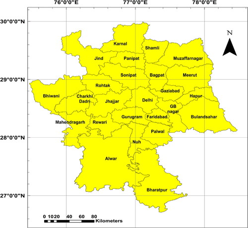
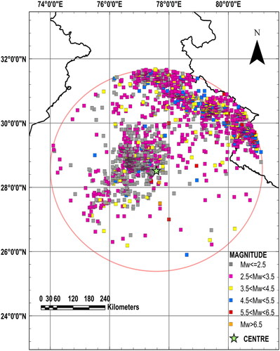
The National Capital Region (NCR) of India consists of the entire National Capital Territory (NCT) of Delhi and 24 districts of its surrounding states like Uttar Pradesh, Haryana, and Rajasthan, as shown in Figure 1, covering an approximate total area of 54,984 km² and more than 46 million people are residing according to Census of India (2011). The NCR has a mixed infrastructure setting of urban, semi-urban, and rural regions. From north to south the region is drained by two major rivers in India, Ganga, and the Yamuna. The NCR is characterized by Indo-Gangetic alluvial plains of quaternary age (Chhabra et al. 2010). The prominent cities of the NCR are Delhi, Faridabad, Gurugram, Noida, Greater Noida, Meerut, Ghaziabad, Bulandsahr, Karnal, Panipat, and Alwar. According to the seismic zonation map of India, the NCR falls under seismic zone-IV (IS-1893 2016). The ongoing developmental infrastructure projects in the region will further result in creating new challenges during seismic events. The seismic resilience of the region can be achieved by a detailed seismic hazard assessment of the region, which is very important for future and existing developmental projects.

Figure 1. Study area, the NCR of India. Source: Author.

2.1. Geological setting

The NCR is characterized by the presence of the Indo-Gangetic plains of quaternary age in the north and east, the extension of the Great Indian Thar desert in the west, and the Aravalli ranges in the south (Mittal et al. 2013). The river Yamuna passes through the eastern part of the Delhi region. The terrain of the region is generally flat except in the central part of the NCR. The formation of a low NNE–SSW trending Delhi ridge is observed. The characteristics of rock formation in the region can be classified from quartzite to quaternary. The geomorphological characteristics of the entire region can be distinguished as (i) the erosional surface which formed the top of denudation hills, (ii) the older alluvial plain (Pleistocene), and (iii) the depositional younger alluvial plain of river Yamuna (Holocene) (Thakur 2013). The rock system of the region has experienced several folding and has undergone multiple processes of metamorphism (Naha et al. 1984). Many faults are found to be trending along NNE-SSW, NE-SW, and WNW-ESE. The stratigraphic succession of the NCR is dated from Precambrian to recent age. Rapid urbanization led to such a dynamic transformation of the geology of the region.

2.2. Seismotectonic setting

The high seismicity of the region is due to the presence of many faults and different geological structures. The major faults and lineaments are georeferenced and digitized using ArcMap 10.5 in the ArcGIS environment (ESRI 2016) based on the seismotectonic atlas, prepared by the Geological Survey of India, and are presented in Figures 2 and 3. In the north-eastern part of the study area, the tectonic belt of young fold mountains of the Himalayas is located and in the southern part, the Proterozoic Delhi fold belt and gneissic batholithic complex are predominant. Highly jointed and Alwar quartzites folding are also observed in surrounding areas and regions to the south of Delhi (Mohanty et al. 2007). The region also shows the presence of the Moradabad fault zone trending along NE-SW direction forming a boundary between two tectonic sub-provinces namely Delhi-Moradabad and Kasganj - Ujhani province (Kumar and Narayan 2020). This tectonic feature is described as a tectonic boundary between the Delhi fold belt and the Vindhya. The northern and south-western boundaries of the Delhi-Moradabad tectonic regime are formed by the Proterozoic Delhi fold belt and the Frontal Fold zone of the Himalaya, respectively (Srivastava et al. 2018). The Delhi-Hardwar ridge can be characterized as the extension of the north-eastward ridge of the Delhi fold belt towards the Himalayas (Chouhan 1975). The Delhi-Haridwar ridge and Monghyr- Saharsa ridge forms the western and eastern margin of the Ganga basin, respectively (Srivastava et al. 2018). In the south-eastern part of Delhi lies a major Rajasthan Great Boundary Fault (GBF) characterized by well-defined Chittaurgarh-Machilpur lineament due to the presence of distinct geomorphic units on either side (Sharma et al. 2003). The presence of the GBF and the Mahendragarh-Dehradun subsurface fault (MDSSF) contributes to the seismicity of the region. The major tectonic features are identified based on previously reported studies (Iyengar and Ghosh 2004; Prakash and Shrivastava 2012) and are presented in Figure 2. Therefore, it can be concluded that the study area is dominated by many seismotectonic features such as faults, structural discontinuities, and lineaments.

Figure 2. Seismotectonic map of the study area. Source: Author.

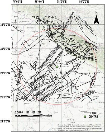
Figure 3. Study area showing (a) the faults, and (b) earthquake events from 1802 to 2020.

Source: Author.

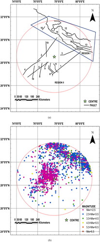
The characterization of seismic source and its behavior is dynamic and varies with the surrounding seismotectonic environment. The study area is divided into two main regions Himalayan region (Region 1) and the NCR of India (Region 2). In the Himalayan region, the events are associated with Main Boundary Thrust (MBT), Main Central Thrust (MCT), and Main Frontal Thrust (MFT) (Mohanty et al. 2007). In the NCR of India, the events are concentrated along Mahendragarh–Dehradun Fault (MDF), Moradabad Fault (MF), and Great Boundary Fault (GBF). For the identification of seismic sources, 19 major faults and lineaments are identified within a 350 km radius from the center of the study area, as shown in Figure 3a, based on past seismic events and seismicity.

2.3. Seismicity

The NCR lies in the proximity of the Himalayas as well as the seismotectonic setting of the region discussed in the previous subsection which indicates the presence of major faults and ridges. The impact of historical and significant past earthquakes which caused great damage to Delhi and its surroundings also corroborates the high seismicity of the region. The 1720 Sohna earthquake (M 6.5) destroyed the walls of the fortress (Red Fort) and many houses in Delhi, and it was followed by 4 to 5 aftershocks per day for 40 days and occasional tremors for 4 to 5 months (Oldham 1883). The occurrence of the 1803 Mathura earthquake (M 6.8) caused damage to Qutab Minar (Oldham 1883) and the 1960 Gurgaon earthquake (M 6.0) caused minor property damages and injuries to about 50 people in Delhi (Singh et al. 2013). Damages to the minarets of Jama Masjid were caused during the 1994 Delhi earthquake (M 4.0) (Iyengar and Ghosh 2004). The geological setting of the NCR can sustain large and amplified ground shaking. The region has been affected many times from the far seismic sources as well as from local seismic activity. It was observed that the damages caused to the buildings and other man-made structures of NCR were severe although the seismic sources were very far away (Mohanty et al. 2007). The tremors of the 1999 Chamoli earthquake (M 6.8), 2011 Pakistan earthquake (M 7.4), 2011 Sikkim earthquake (M 6.9), 2015 Nepal earthquake (M 7.8), and many other earthquakes were strongly felt in the region. Recently, in the year 2020, the region has experienced more than ten earthquakes (M > 4.0) and its epicenters are in and around the NCR. As the region is densely populated and has many critical infrastructures and world heritage monuments, an increase in seismic activity poses a threat to both life and property.

3. Preparation of earthquake catalogues and their homogenization

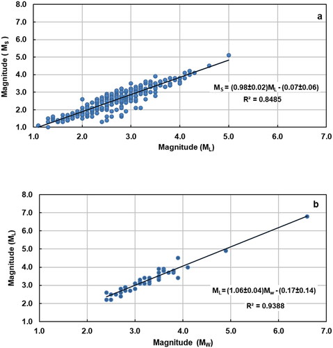
The preparation of the earthquake catalogue is considered the most important step for PSHA. A comprehensive earthquake catalogue is prepared for the study area considering the radius of 350 km centered on Shiv Nadar University (28°31ʼ29ʼʼ N, 77°34ʼ28ʼʼE). Earthquake data have been collected from national as well as international databases including the National Centre for Seismology (NCS), Bhukosh-Geological Survey of India (GSI), India Meteorological Department (IMD), Institute of Seismological Research (ISR), International Seismological Centre (ISC-GEM Earthquake Catalogue 2021), United States Geological Survey National Earthquake Information Centre (USGS NEIC), and many peer-reviewed research articles (Oldham 1883; Chouhan 1975; Naha et al. 1984; Sharma et al. 2003; Iyengar and Ghosh 2004; Mohanty et al. 2007; Prakash and Shrivastava 2012; Mittal et al. 2013; Thakur 2013; IS-1893 2016; Srivastava et al. 2018; Kumar and Narayan 2020). A total number of 2034 events are collected from 1802 to 2020 with detailed information about the date and time of occurrence, magnitude, hypocentral depth, and location with specified coordinates (Figure 3b).

The earthquake catalogue comprises earthquakes recorded on different magnitude scales such as surface-wave magnitude (M_s), moment magnitude (M_w), body-wave magnitude (M_b), and local magnitude (M_L) with a majority of events recorded on the moment and local magnitude scales. Most of the data points are originally recorded in terms of moment magnitude and local magnitude. The magnitudes are homogenized to a unified and common magnitude scale i.e., moment magnitude (M_w) by using the orthogonal regression approach (Orthogonal Distance Regression) (Das et al. 2012; Lindholm et al. 2016). Limited data points are available for the body-wave magnitude scale which are found to be common with either M_L or M_s scales. There are 297 and 53 data points for the orthogonal regression between M_L and M_s (Figure 4a) and M_w and M_L (Figure 4b), respectively. So, the following relations are obtained based on orthogonal regression and used for conversion of M_s and M_L to M_w (Equations (1)(1) $$M_S=(0.98\pm 0.02)M_L-(0.07\pm 0.06)$$(1) and (2)(2) $$M_L=(1.06\pm 0.04)M_W-(0.17\pm 0.14)$$(2) ). (1) $$M_S=(0.98\pm 0.02)M_L-(0.07\pm 0.06)$$(1) (2) $$M_L=(1.06\pm 0.04)M_W-(0.17\pm 0.14)$$(2)

Figure 4. Linear regression relation (a) between M_L and M_S, and (b) between M_W and M_L. Source: Author.

4. Declustering of earthquake catalogues

The earthquake catalogue obtained for the study region comprises of mainshocks along with their foreshocks and aftershocks. Both foreshock and aftershock depend spatially and temporally on the mainshock. As mutually exclusive events are considered in the probabilistic seismic hazard analysis of a region, it is important to remove the dependent events from the prepared earthquake catalogue. In the present study, the dependent events are separated from the main events by declustering of earthquake data based on Reasenberg declustering algorithm (Reasenberg 1985; Wiemer 2001; Zhuang et al. 2002) using MATLAB based opensource software ZMAP (Wiemer 2001; Vipin et al. 2013; Telesca et al. 2016; Sinha and Sarkar 2020; Borah and Kumar 2021). The parameters associated with the Reasenberg declustering algorithm are minimum time interval (τ_min) and maximum time interval (τ_max) for the occurrence of the next earthquake event with a certain probability p. Relationship between these three parameters used in the declustering algorithm is expressed in Equation (3)(3) $$\tau =-\hspace{0.17em}\text{ln}\hspace{0.17em}(1-p1)t/{10}^{2(\Delta M-1)/3}$$(3) . (3) $$\tau =-\hspace{0.17em}\text{ln}\hspace{0.17em}(1-p1)t/{10}^{2(\Delta M-1)/3}$$(3)

Where ΔM is the difference between maximum and minimum magnitude, t is the time interval. A total of 14 clusters of earthquakes are identified and 90 dependent events out of 2034 are found. A map of the control region showing 1944 mutually exclusive seismic events after the declustering of earthquake data is shown in Figure 5.

Figure 5. A map of the control region showing 1944 mutually exclusive seismic events.Source: Author.

5. Analysis of completeness of seismic data

The homogenized earthquake data is further analyzed to check the completeness of the data set in the given time interval based on the methods proposed by Stepp (Stepp 1972; Khan and Kumar 2018). The data is grouped into several magnitude classes and each class is modeled as a point process in time to obtain the variance of the sample mean. In this procedure, the number of earthquakes occurring per decade is classified into magnitude ranges of 3.0 ≤ M_w < 4.0, 4.0 ≤ M_w < 5.0, 5.0 ≤ M_w < 6.0, M_w ≥ 6.0. The earthquake sequence is modeled by assuming Poisson's distribution to evaluate the variance of the sample mean. If k₁, k₂, k₃, …, and k_n are the number of earthquakes per unit time interval, then an unbiased estimate of the mean rate per unit time interval of the sample will be, (4) $$\lambda =\frac{1}{n}\sum _1^n{k}_i$$(4)

And its variance will be given by, (5) $${\sigma }_{\lambda }^2=\frac{\lambda }{n}$$(5)

Where n is the number of unit time intervals (1 year).

Now the standard deviation of the mean number of annual events will be calculated as (6) $${\sigma }_{\lambda }=\sqrt{\frac{\lambda }{T}}$$(6)

Where T is the sample length in years (Stepp 1972). The standard deviation versus time intervals is plotted for every magnitude class as shown in Figure 6a and 6b. If the data for a given magnitude interval is completed, then the plotted points will give a straight line parallel to the slope of 1/√T. Fig. 6a and b reveal that completeness of 20, 40, 50, and 80 years for the region I and 20, 60, 90, and 100 years for region II from the year 2020 in the moment magnitude classes of 3-4, 4-5, 5-6 and > 6, respectively (Table 1).

Figure 6. Check for the completeness of seismic data for (a) Region I, and (b) Region II. Source: Author.

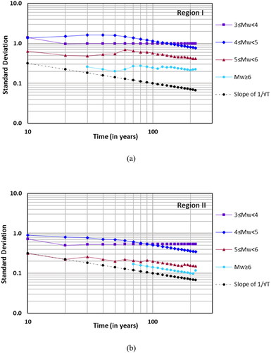
Table 1. Completeness of homogeneous earthquake catalogue with respect to time.

	Approximate years of completeness
Magnitude (Mw)	Region I	Region II
3.0 ≤ Mw < 4.0	20	20
4.0 ≤ Mw < 5.0	40	60
5.0 ≤ Mw < 6.0	50	90
Mw ≥ 6.0	80	100

6. Estimation of seismic parameters a, b and M_C

After checking the completeness of the earthquake catalogue of the study area temporally, it is also necessary to evaluate the magnitude of completeness (M_C). M_C is defined as the lowest magnitude at which 100% of the seismic events in a space-time volume are identified (Wiemer and Wyss 2000). Different methods are used in the past for the estimation of M_C values, such as the maximum curvature method, fixed minimum magnitude observed (M_min), the goodness of fit (M_min90 and M_min95), the best combination of M_min90 and maximum curvature, entire magnitude range, and bootstrap method (Anbazhagan et al. 2019). In the present study, the values of M_C for regions I and II are determined using the maximum curvature method (Figures 7a and 7b) and the values are presented in Table 2. The obtained Mc values for regions I and II are 3.0 and 2.1 respectively. So, taking that into account, 3.0 Mw has been adopted as minimum magnitude (m₀) for both the regions for further analysis (Anbazhagan et al., 2015).

Table 2. List of calculated seismic parameters and its comparison with reported values for the region.

Parameter		NCS-MoES (2016)	NDMA (2010)	Iyengar and Ghosh (2004)	Present study
Region I	a	2.64 ± 0.16	Not reported	Not reported	2.47 ± 0.21
	b	0.59 ± 0.03	Zone 2: .73 ± 0.04 Zone 3: .78 ± 0.04	0.78	0.67 ± 0.04
	Mc	4.0	Not reported	Not reported	3.00
Region II	a	0.62 ± 0.08	Not reported	Not reported	1.48 ± 0.20
	b	0.42 ± 0.12	Zone 28: .81±.06	0.87	0.58 ± 0.04
	Mc	3.0	Not reported	Not reported	2.10

The seismic activity of the region is estimated in terms of the recurrence rate of earthquakes for the different range of magnitudes using an empirical relationship in Equation (7)(7) $${\hspace{0.17em}\text{log}}_{10\hspace{0.17em}}N=a-b{M}_W$$(7) proposed by Gutenberg and Richter (1944). It is one of the simplest and widely used approaches for the quantification of seismic parameters a and b of a region (Sitharam and Sil, 2014; Anbazhagan et al. 2015). (7) $${\hspace{0.17em}\text{log}}_{10\hspace{0.17em}}N=a-b{M}_W$$(7)

N denotes the number of earthquakes greater than or equal to magnitude M_w per year, a represents seismic activity and b is known as a tectonic parameter. Based on the magnitude of completeness seismic parameters are estimated using GR recurrence law. The total number of earthquakes greater than magnitude 3.0 is 638, i.e., 461 in the region I and 177 in region II. The value of a and b are determined for both regions and it is compared with the other reported past studies as shown in Table 2 and Figure 8.

Figure 7. Estimation of Mc, a, and b parameters for (a) Region I, and (b) Region II. Source: Author.

Figure 8. Gutenberg - Richter relation for the Region I and II. Source: Author.

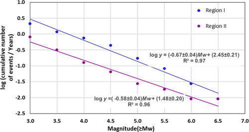
It is observed that the value of b is lower for the Himalayan region as compared to the NCR of India, and this is because the seismic parameter b is related to the occurrence of large to smaller seismic events and the Himalayan region experiences earthquakes of higher magnitude as compared to the NCR, where lower magnitude earthquakes are predominant.

7. Fault deaggregation

19 major faults are identified in the study area and any site in the study area will be subjected to ground shaking from any of these seismic sources. The recurrence relationship developed earlier is related to the entire study region and it is not specific for a particular fault. To differentiate seismic activity rates among different faults and to distinguish near seismic sources from distant sources, the development of fault-level recurrence relation is essential. The approach to developing a frequency magnitude relationship for individual seismic sources can lead to discrepancies in results due to the scarcity of seismic activity rates. Another approach is to calculate the value of b by determining the slip rate of individual faults, but the estimation of slip rate is also difficult as slip values of all the faults are not recorded for historical events. The regional recurrence of the NCR is disaggregated into individual fault recurrence by using the method suggested by Raghukanth and Iyengar (2006), based on the heuristic principle of conservation of seismic activity stating the regional seismicity defined as the number of earthquakes per year with m > m₀, should be equal to the sum of the number of earthquakes occurring on individual faults (Raghukanth and Iyengar 2006). (8) $$N(m_0)=\sum N_i(m_0)\left(i=1,\mathrm{}2,\mathrm{}3,\mathrm{}4,\mathrm{}\dots ,\mathrm{}19\right)$$(8)

In the determination of N_i(m₀), two assumptions are important in terms of fault length weighing factor (α_i)and earthquake events weighing factor (χ_i). The first assumption is that the longer the fault, the higher is the capacity of producing a greater number of earthquakes of smaller magnitude m₀ than the faults of shorter length. Therefore, N_i(m₀) is proportional to the length of the fault and this observation leads to the weighing factor ${\alpha }_i=L_i/\sum L_i,$ L_i is equal to the length of the fault i. It is also observed that irrespective of the length of the fault, a shorter fault may be more active to produce smaller magnitudes of earthquakes than a longer fault. The second assumption is that the future seismic activity will remain similar to past activity, at least for the short term. So, seismic activity needs to be related to the number of past events associated with each fault in the earthquake catalogue as depicted in Figure 9. Another weighing factor, χ_i, is defined as the ratio of the number of earthquakes associated with fault i to the total number of earthquakes in the region. The final recurrence relation for a fault i is given as (9) $$N_i(m_0)=0.5({\alpha }_i+{\gamma }_i)N(m_0)$$(9)

Figure 9. Earthquakes associated with each fault. Source: Author.

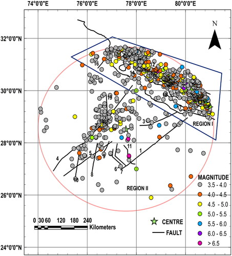
In the PSHA of NCR, 19 seismic sources have been identified, the details of each fault in terms of length of the fault, shortest hypocentral distances from Shiv Nadar University, Delhi-NCR, India, the maximum magnitude of earthquake associated with each fault, number of earthquake events occurred in the proximity of each fault and weighting factors for each fault are given in Table 3.

Table 3. Deaggregation of faults.

Fault ID	Fault name	Length of fault (Km)	Mmax	Shortest hypocentral distance (Km)	No. of earthquake associated	αi	χi	Average of αi and χi
1	Great Boundary Fault (GBF)	320	7.3	114	6	0.17	0.07	0.12
2	Mahendraghar-Dehradun fault (MD)	295	5.7	82	27	0.15	0.30	0.23
3	Moradabad	170	6.1	59	5	0.08	0.05	0.07
4	Chahapoli	215	5.7	137	6	0.11	0.07	0.09
5	Sabi Fracture	200	4.9	74	8	0.10	0.09	0.09
6	Near Mathura	92	4.8	92	3	0.05	0.03	0.04
7	Fault Parallel to no. 6	115	4.8	66	3	0.06	0.03	0.04
8	Fault left of Alwar	126	4.9	127	6	0.07	0.07	0.07
9	Fault near Alwar	53	4.9	84	6	0.03	0.07	0.05
10	Fault near Jaipur	117	5.1	205	5	0.06	0.05	0.05
11	Mathura	101	7.3	63	4	0.05	0.04	0.04
12	Main Central Thrust (MCT)	355	7.3	223	174	0.34	0.54	0.44
13	North Almora Thrust (NAT)	279	7.1	210	49	0.16	0.15	0.15
14	Main Boundary Thrust (MBT)	464	6.5	157	21	0.32	0.06	0.19
15	Alakananda	50	7.3	219	51	0.03	0.16	0.09
16	Ropar	37	5.5	260	3	0.02	0.01	0.01
17	Near Ramgarh	38	6.5	230	5	0.02	0.02	0.02
18	South Almora Thrust (SAT)	193	6.5	211	15	0.11	0.05	0.08
19	Sohna Fault	107	5.4	75	18	0.06	0.20	0.13

To obtain the maximum possible earthquake (M_max) that each fault can produce, the conventional incremental method is adopted (Gupta 2002; Anbazhagan et al. 2015). The observed maximum magnitude ($M_{\mathit{obs}}^{\max }$) associated with each seismic source is increased by 0.5 units based on the obtained b values (Anbazhagan et al. 2015; Anbazhagan et al. 2019). The details of each fault in terms of the total length and M_max with an increment of 0.5 units higher than the magnitude reported in the past are shown in Table 3 (Raghukanth and Iyengar 2006).

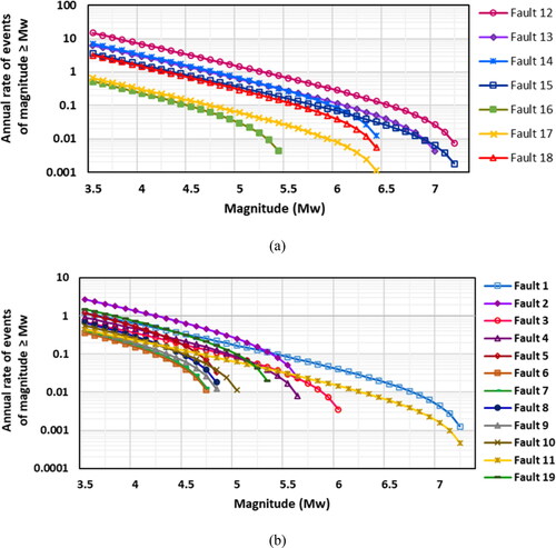
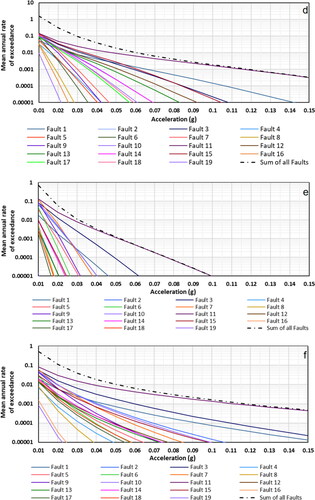
The b value of each fault is equal to the b value of the region in which the fault is located. The equation obtained is: (10) $$N_i(m_0)=N_i(m_0)[1-\{(1-e^{-\beta (m-m_0)})/(1-e^{-\beta (m_{\max }-m_0)})\}$$(10) m₀ is the value of threshold magnitude, m_max is the maximum potential magnitude of the fault i and β = 2.303 b. The final individual fault level recurrence relation is shown in Figure 10a and 10b.

Figure 10. Fault level recurrence relation for (a) Region I, and (b) Region II. Source: Author.

8. Probabilistic seismic hazard assessment

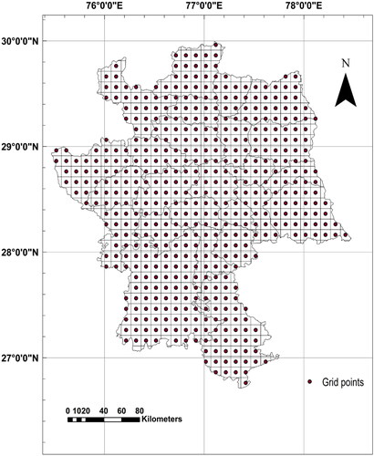
The entire study area is divided using a grid of 10 km × 10 km with a total of 524 grid points, as shown in Figure 11, for the estimation of seismic hazard at the bedrock level for the NCR of India. In this study, every grid point is selected as a site of interest. With the help of ArcGIS 10.5, the shortest and longest distances from each grid point to all active faults present in the study area are estimated. MATLAB programming is used for all computational purposes and probabilistic seismic hazard assessment to calculate the ground motion parameters.

Figure 11. Grids used for PSHA in the NCR of India. Source: Author.

The number of earthquake events that occur on a fault is assumed to follow a stationary Poisson process, and the probability of a random variable Y exceeding level a, in a period T year at a site can be represented by the annual rate of exceedance µ_a. (11) $$P(Y>a)=1-e^{-{\mu }_{a}T}$$(11)

The expression for µ_a is given as (12) $${\mu }_a=\sum _{i=1}^K{N}_i(m_0){\int }_m{\int }_{r}P(Y>a)|m,r)p_{R|M}(r|m)p_M(m)\mathit{drdm}$$(12)

K is the number of faults present in the study region, $p_M\left(m\right)$ is the probability density function of magnitude, $p_{\left.R\right|M}\mathrm{}\left(rm\right)$ is the probability density function of hypocentral distance and the conditional probability of exceedance of the ground motion parameter is denoted by $P(Y>a\mathrm{}|\mathrm{}m,r).$ The return period for the corresponding ground motion value is given by the reciprocal of the annual probability of exceedance.

8.1. Uncertainty in magnitude

Seismic sources present in a region are capable of producing earthquakes of different sizes and smaller magnitude earthquakes have a higher frequency than the earthquake of greater magnitude. A seismic source is assumed to cause an earthquake of magnitude as a random variable distributed in the range of M_min (m₀) to M_max (m_max), following Equation (13)(13) $${\hspace{0.17em}\text{log}\hspace{0.17em}}_{10}N(m)=a-bm$$(13) for the recurrence relation. (13) $${\hspace{0.17em}\text{log}\hspace{0.17em}}_{10}N(m)=a-bm$$(13)

The probability density function for magnitude uncertainty of all 19 faults, $p_M\left(m\right),\mathrm{}$ is given in Equation (14)(14) $$p_M(m)=\beta e^{-\beta (m-m_0)}/(1-e^{-\beta (m_{\max }-m_0)})$$(14) (14) $$p_M(m)=\beta e^{-\beta (m-m_0)}/(1-e^{-\beta (m_{\max }-m_0)})$$(14)

Here m₀ ≤ m ≤ m_max and β = 2.303 b (Iyengar and Ghosh 2004).

8.2. Uncertainty in hypocentral distance

Another uncertainty exists in terms of the source-to-site distance in the PSHA. It is assumed that all points on an active fault have equal potential to get ruptured and to produce earthquakes of significant magnitude. Therefore, the hypocentral distance R is treated as a random variable and it depends on the relative orientation of the fault with respect to the site (Kramer 1996). In this study, the faults in the study region are the linear sources and the occurrence of a seismic event can take place at any point along the fault. The probability distribution function of the hypocentral distance R can be expressed as Equation (15)(15) $$p_{R|M}(r|m)=\frac{r}{L\sqrt{r^2-r_{\min }^2}}$$(15) . (15) $$p_{R|M}(r|m)=\frac{r}{L\sqrt{r^2-r_{\min }^2}}$$(15)

Where L is the length of the fault and r_min is the minimum hypocentral distance from the site. Equation (15)(15) $$p_{R|M}(r|m)=\frac{r}{L\sqrt{r^2-r_{\min }^2}}$$(15) is applied for the calculation of the probability density function of uncertainty in hypocentral distances for all the seismic sources present within the study region and is applicable when the fault is located completely to one side of the site of interest (Kramer 1996). In most cases, the faults extend on both sides of the seismic source, and the probability for the total fault is estimated by the summation of the product of conditional probabilities of both sides and a fraction of corresponding sides.

8.3. Attenuation relationships

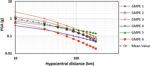
An attenuation relationship, also called ground motion prediction equation (GMPE), can be derived by regression analysis of past recorded earthquake data of the region and it depends on several factors like the geometry of the seismic source, the magnitude of earthquake event, corresponding source to site distance, path characteristics, and local site conditions. The knowledge of site-specific attenuation relation is very important for evaluation of ground motion parameter (Singh et al. 1996), but in case of limited data, one can use the previously developed attenuation models for the region or models based on similar tectonic features as shown by various researchers such as Nath and Thingbaijam (2012), Anbazhagan et al. (2015) and Anbazhagan et al. (2019). The development of attenuation relationship for the entire NCR of India has limitations due to lack of strong-motion data, correct epicentral distances, and range of earthquake magnitude. Very few ground motion prediction equations are available for Northern India (Sharma 1998; Iyengar and Ghosh 2004; Rao and Rathod 2014) and Himalayan region (Aman et al. 1995; Singh et al. 1996; NDMA 2010; Joshi et al. 2012; Ahmad and Singh 2016, etc.). However, there is no specific GMPE derived for the entire NCR. In the present study, six different ground motion equations suggested by Bajaj and Anbazhagan (2019), Rao and Rathod (2014), Joshi et al. (2012), Iyengar and Ghosh (2004), Ambraseys and Bommer (1991), and Cornell et al. (1979) are used. The average of the ground motion parameter values, calculated from the following six GMPEs, are used to determine peak ground acceleration (PGA) values of the NCR of India. Figure 12 shows attenuation relations for PGA versus hypocentral distance at magnitude 7.0 represented for all six GMPEs and their average.

Figure 12. PGA vs. Hypocentral distance for M_w 7.0. Source: Author.

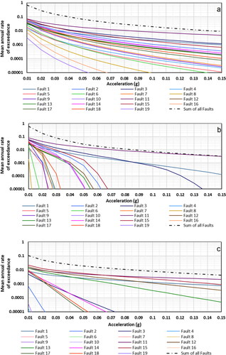
For individual ground motion prediction equation (GMPE), seismic hazard curves at Shiv Nadar University of the study region are shown in Figure 13a through Figure 13f. The GMPEs used in this study are expressed below.

Figure 13. Seismic hazard curves generated for SNU site using (a) GMPE 1, (b) GMPE 2, (c) GMPE 3, (d) GMPE 4, (e) GMPE 5, and (f) GMPE 6. Source: Author.

The attenuation relation (GMPE 1) developed by Bajaj and Anbazhagan (2019) for the Himalayan region is expressed as (16) $$\text{ln}\hspace{0.17em}Y=a_1+a_2(M-6)+a_3{(9-M)}^2+a_4\hspace{0.17em}\text{ln}\hspace{0.17em}R+a_m\hspace{0.17em}\text{ln}\hspace{0.17em}R(M-6)+a_{7}R+\sigma$$(16) ln Y is the logarithm of ground motion, M is magnitude and R is hypocentral distance. The value of standard deviation, σ is equal to 0.817. The regression coefficients are a₁, a₂, a₃, a₄, a_m (for M_w < 6.0 and R < 300, a_m in Equation (16)(16) $$\text{ln}\hspace{0.17em}Y=a_1+a_2(M-6)+a_3{(9-M)}^2+a_4\hspace{0.17em}\text{ln}\hspace{0.17em}R+a_m\hspace{0.17em}\text{ln}\hspace{0.17em}R(M-6)+a_{7}R+\sigma$$(16) is a₅, otherwise a_m is a₆) and a₇ and corresponding values are 1.071, −0.257, −0.184, −0.479, 0.078 (a₅), 0.076 (a₆), and −0.0085, respectively.

Rao and Rathod (2014) performed regression analysis using 1,650 data to obtain the attenuation relation (GMPE 2) for rock site condition as a function of magnitude and distance given in Equation (17)(17) $${\hspace{0.17em}\text{log}}_{10\hspace{0.17em}}(\mathit{PGA})=c_1+c_2(M_W-6)+c_3{(M_W-6)}^2+c_{4}R+c_5{\hspace{0.17em}\text{log}\hspace{0.17em}}_{10}R+{\hspace{0.17em}\text{log}\hspace{0.17em}}_{10}\epsilon$$(17) . (17) $${\hspace{0.17em}\text{log}}_{10\hspace{0.17em}}(\mathit{PGA})=c_1+c_2(M_W-6)+c_3{(M_W-6)}^2+c_{4}R+c_5{\hspace{0.17em}\text{log}\hspace{0.17em}}_{10}R+{\hspace{0.17em}\text{log}\hspace{0.17em}}_{10}\epsilon$$(17)

The unit of PGA is g, M_w is moment magnitude, R is the hypocentral distance expressed in km, and the values of regression coefficients c₁, c₂, c₃, c_4, and c₅ are 0.66845, 0.49908, −0.04665, −0.00257, and −0.85968, respectively. The value of the standard deviation of random error σ (log 10ε) is 0.1118.

Joshi et al. (2012) derived ground motion prediction equation (GMPE 3) by using data from 8 stations installed in the Pithoragarh region of Kumaon Himalaya. The ground motion prediction model is expressed in Equation (18)(18) $$\text{ln}\hspace{0.17em}(\mathit{PGA})=a_1+a_2{M}_W+a_3\hspace{0.17em}\text{ln}\hspace{0.17em}{r}_{\mathit{hypo}}+a_4\hspace{0.17em}\text{ln}\hspace{0.17em}(r_{\mathit{epi}}+15)$$(18) and the range of hypocentral distance in this study varies between 10 km to 100 km. (18) $$\text{ln}\hspace{0.17em}(\mathit{PGA})=a_1+a_2{M}_W+a_3\hspace{0.17em}\text{ln}\hspace{0.17em}{r}_{\mathit{hypo}}+a_4\hspace{0.17em}\text{ln}\hspace{0.17em}(r_{\mathit{epi}}+15)$$(18)

The value of PGA is in Gal, and the coefficients a₁ = −5.8, a₂ = 2.62, a₃ = −0.16, a₄ = −1.33 and σ = 0.42.

Iyengar and Ghosh (2004) proposed attenuation relation (GMPE 4) for Delhi City, which is used in the present study, is as follows in Equation (19)(19) $${\hspace{0.17em}\text{log}}_{10}(y)=C_1+C_{2}M-B{\hspace{0.17em}\text{log}}_{10}(r+e^{C_{3}M})+P\sigma$$(19) . (19) $${\hspace{0.17em}\text{log}}_{10}(y)=C_1+C_{2}M-B{\hspace{0.17em}\text{log}}_{10}(r+e^{C_{3}M})+P\sigma$$(19)

Where C₁ = −1.5232, C₂ = 0.3677, C₃ = 0.41, B = 1.0047 and σ = 0.2632. The value of P equals to 0 for the median and 1 for 84 percentile value of PGA.

The ground motion model (GMPE 5) proposed by Ambraseys and Bommer (1991) can be represented as Equation (20)(20) $$\text{log}\hspace{0.17em}(a)=\alpha +\beta M-\hspace{0.17em}\text{log}\hspace{0.17em}r+br$$(20) . (20) $$\text{log}\hspace{0.17em}(a)=\alpha +\beta M-\hspace{0.17em}\text{log}\hspace{0.17em}r+br$$(20) a is in g, α = −0.87, β = 0.217, b = −0.00117 and σ = 0.26

The ground motion equation (GMPE 6) proposed by Cornell et al. (1979), is (21) $$\text{ln}\hspace{0.17em}(Ap)=a+b{M}_L+c\hspace{0.17em}\text{ln}\hspace{0.17em}(R+25)$$(21)

A_p is expressed in cm/sec², a = 6.74, b = 0.859, c = −1.80 and σ = 0.57

8.4. Determination of temporal uncertainty

Earthquakes occur randomly from time to time, and therefore, temporal uncertainties must be considered in the assessment of seismic hazards. The probability of occurrence of an earthquake event in a given period can be calculated considering the distribution of earthquakes with time. The number of seismic events that occur on a fault and the temporal occurrence of earthquakes can be determined with the help of the stationary Poisson model (Iyengar and Ghosh 2004). The probabilities of exceedance of specific ground motion parameter a for period T is expressed as Equation (22)(22) $$P(Y>a)=1-e^{-{\mu }_{a}T}$$(22) that represents the relation between the mean annual rate of exceedance (µ_a) and period (T) (22) $$P(Y>a)=1-e^{-{\mu }_{a}T}$$(22)

The values of annual mean exceedance µ_a are calculated, in this study, for 2% and 10% probabilities of exceedance in 50 and 100 years.

9. Seismic hazard mapping and comparison

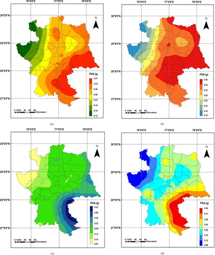
The seismic hazard curves are prepared for all the 19 faults and then combined to quantify the value of aggregate hazard at the sites of interest. The entire NCR is divided into 524 grids of a grid size of 10 km x 10 km. After estimating the value of the mean annual rate of exceedance (µ_a) at each of these sites, PGA at rock level for 2% and 10% probability of exceedance in 50 and 100 years are computed using the six most suitable attenuation relationships and their average. The seismic hazard map for NCR of India is generated and presented in Figure 14a–d using the average PGA value estimated at each site corresponding to 2% and 10% probability of exceedances for both 50 years and 100 years. The PGA values estimated using the average values of all six GMPEs are 0.12 to 0.37 g, 0.15 to 0.40 g, 0.07 to 0.33 g, and 0.08 to 0.35 g for 2% probability of exceedance in 50 years, 2% probability of exceedance in 100 years, 10% probability of exceedance in 50 and 10% probability of exceedance in 100 years, respectively (Mehta and Thaker 2020). The eastern and south-eastern portions of the study region are exhibiting high PGA values (Figure 14a–d). A similar spatial pattern is also reported by some previous studies like Sharma et al. (2003), Sharma and Wason (2004), Sarkar and Shankar (2017) for the same study area. The PGA maps reveal that the south-eastern part of the study area is more affected due to the presence of Great-Boundary fault (GBF), Mathura fault, and Moradabad faults. The eastern part of the study area also indicated high PGA values due to its vicinity to the Himalayan zone, which is associated with high seismicity due to the presence of numerous faults and lineaments (Figure 14a–d).

Figure 14. PGA at rock level for (a) 2% probability of exceedance in 50 years, (b) 2% probability of exceedance in 100 years, (c) 10% probability of exceedance in 50 years, and (d) 10% probability of exceedance in 100 years. Source: Author.

The results obtained from the present study and its comparison with the results reported on the seismic hazard studies carried out for the Delhi region (Iyengar and Ghosh 2004; Rao and Rathod 2014; NCS-MoES 2016; Sarkar and Shankar 2017) are given in Table 4. The comparison with Sharma et al. (2003) cannot be tabulated as they reported the PGA values for 20% probability of exceedance in 50 years. The values obtained in the present study are on the higher end as compared to the previous study. The PGA value estimation depends upon the factors like selection of appropriate GMPE, seismic sources, and associated seismic parameters. The use of under-predictive GMPEs may be the reason for lower PGA values by the previous studies.

Table 4. Comparison of PGA values estimated in the present study with past results.

	PGA (g) value
	2% probability of exceedance in		10% probability of exceedance in
	50 years	100 years	50 years	100 years
Present Study	0.12 − 0.37	0.15 − 0.40	0.07 − 0.33	0.08 − 0.35
Sarkar and Shankar (2017)	0.00 − 0.64	Not Reported	0.00- 0.37	Not Reported
NCS-MoES (2016)	0.08 − 0.16	Not Reported	0.04 − 0.08	Not Reported
Rao and Rathod (2014)	0.14 − 0.23	Not Reported	Not Reported	Not Reported
Iyengar and Ghosh (2004)	0.19 − 0.24	Not Reported	Not Reported	Not Reported

The PGA values estimated using the average values of all six GMPEs are 0.12 to 0.37 g, 0.15 to 0.40 g, 0.07 to 0.33 g, and 0.08 to 0.35 g for 2% probability of exceedance in 50 years, 2% probability of exceedance in 100 years, 10% probability of exceedance in 50 and 10% probability of exceedance in 100 years, respectively. The seismic hazard maps for NCR developed in the present study will serve as a significant input in sustainable urban planning, city planning for critical and lifeline infrastructures, preparedness, and mitigation planning, designing, and constructing earthquake-resistant structures as well as in hazard and risk mitigation and management.

10. Conclusions

A comprehensive probabilistic seismic hazard assessment for the NCR of India at the bedrock level is carried out in this study. The faults and geological discontinuities are identified with the help of Seismotectonic Atlas (SEISAT) maps and the seismotectonic map of the study area is prepared by using ArcGIS 10.5. The regional seismicity of the area is due to the presence of major 19 faults of different lengths and maximum potential magnitude. By using the earthquake data from 1802 to 2020, regional recurrence for both regions is obtained. The entire area is divided into 524 grids and for each grid PGA value at bedrock level is determined with the help of suites of suitable ground motion prediction equations (GMPEs).

For every grid point, hazard curves are also generated. The final seismic hazard mapping is based on the PGA values calculated based on the suite of suitable ground motion prediction equations. In this study, it is found that the resulting PGA value of the region varies in the range of 0.12 to 0.37 g, 0.15 to 0.40 g, 0.07 to 0.33 g, and 0.08 to 0.35 g for 2% probability of exceedance in 50 years, 2% probability of exceedance in 100 years, 10% probability of exceedance in 50 and 10% probability of exceedance in 100 years, respectively. This probabilistic seismic hazard analysis reveals that the eastern and south-eastern regions of the study area are more vulnerable to seismic hazards. The present study can be considered as a comprehensive assessment of seismic hazards for NCR India, but it has its limitations. Seismic hazard assessment itself consists of many inherent uncertainties, all the uncertainties could not be considered in the present study although major uncertainties in terms of magnitude and epicentral distances have been addressed. The study area consists of many major and minor seismic sources like faults, lineaments, thrusts, for the present work only major faults are considered based on literature review and historical earthquake occurrence. Limitations of the study also lie in the lack of geotechnical, geological, seismological, and other seismic hazard-related data. These findings will provide greater insights and input for the design and construction of earthquake-resistant structures and in decision-making for disaster risk reduction.

Author contributions

Laxmi Gupta: Methodology, Formal analysis, Software, Resources, Investigation, Data curation, Validation, Visualization, Writing - Original Draft. Navdeep Agrawal: Methodology, Formal analysis, Software, Data curation, Validation, Writing - Original Draft. Jagabandhu Dixit: Conceptualization, Methodology, Software, Validation, Resources, Supervision, Project administration, Writing - Review & Editing.

Disclosure statement

No potential conflict of interest was reported by the authors.

Data availability statement

The authors confirm that some portion of the data supporting the findings of this study is available within the article. Some of the raw data were generated at our laboratory and derived data supporting the findings of this study are available from the corresponding author [J.D.], upon reasonable request.

References

- Agrawal N, Gupta L, Dixit J. 2021. Assessment of the socioeconomic vulnerability to seismic hazards in the national capital region of India using factor analysis. Sustainability. 13(17):9652.
- Ahmad R, Singh RP. 2016. Attenuation relation predicted observed ground motion of Gorkha Nepal earthquake of April 25, 2015. Nat Hazards. 80(1):311–328.
- Ahmad RA, Singh RP, Adris A. 2017. Seismic hazard assessment of Syria using seismicity, DEM, slope, active faults and GIS. Remote Sens Appl: Soc Environ. 6:59–70.
- Aman A, Singh UK, Singh RP. 1995. A new empirical relation for strong seismic ground motion for the Himalayan region. Curr Sci. 69(9):772–777.
- Ambraseys NN, Bommer JJ. 1991. The attenuation of ground accelerations in Europe. Earthquake Eng Struct Dyn. 20(12):1179–1202.
- Anbazhagan P, Bajaj K, Matharu K, Moustafa SS, Al-Arifi NS. 2019. Probabilistic seismic hazard analysis using the logic tree approach–Patna district (India. Nat Hazards Earth Syst Sci. 19(10):2097–2115.
- Anbazhagan P, Bajaj K, Patel S. 2015. Seismic hazard maps and spectrum for Patna considering region-specific seismotectonic parameters. Nat Hazards. 78(2):1163–1195.
- Bajaj K, Anbazhagan P. 2019. Regional stochastic GMPE with available recorded data for active region–Application to the Himalayan region. Soil Dyn Earthquake Eng. 126:105825.
- Baltay AS, Hanks TC, Abrahamson NA. 2017. Uncertainty, variability, and earthquake physics in ground‐motion prediction equations. Bull Seismol Soc Am. 107(4):1754–1772.
- Bhukosh, Geological Survey of India 2021 [accessed: 2021 June 26] https://bhukosh.gsi.gov.in/Bhukosh/Public.
- Bommer JJ. 2002. Deterministic vs. probabilistic seismic hazard assessment: an exaggerated and obstructive dichotomy. J Earthquake Eng. 6(sup001):43–73.
- Borah N, Kumar A. 2021. Studying and comparing the declustered EQ catalogue obtained from different methods for Guwahati region NE India. In Geohazards. Singapore: Springer; p. 577–590.
- Bungum H, Lindholm CD, Mahajan AK. 2017. Earthquake recurrence in NW and central Himalaya. J Asian Earth Sci. 138:25–37.
- Census of India 2011. Provisional population totals. New Delhi: Office of the Registrar General and Census Commissioner
- Chhabra A, Manjunath KR, Panigrahy S. 2010. Non-point source pollution in Indian agriculture: Estimation of nitrogen losses from rice crop using remote sensing and GIS. Int J Appl Earth Obs Geoinf . 12(3):190–200.
- Chouhan RKS. 1975. Seismotectonics of Delhi region. Proc. Indian Nat. Sci. Acad. 41:429–447.
- Cornell CA. 1968. Engineering seismic risk analysis. Bull Seismol Soc Am. 58(5):1583–1606.
- Cornell CA, Banon H, Shakal AF. 1979. Seismic motion and response prediction alternatives. Earthquake Eng Struct Dyn. 7(4):295–315.
- Crowley H, Bommer JJ, Pinho R, Bird J. 2005. The impact of epistemic uncertainty on an earthquake loss model. Earthquake Eng Struct Dyn. 34(14):1653–1685.
- Das R, Wason HR, Sharma ML. 2012. Magnitude conversion to unified moment magnitude using orthogonal regression relation. J Asian Earth Sci. 50:44–51.
- Deligiannakis G, Papanikolaou ID, Roberts G. 2018. Fault specific GIS based seismic hazard maps for the Attica region, Greece. Geomorphology. 306:264–282.
- Dixit J, Dewaikar DM, Jangid RS. 2012. Soil liquefaction studies at Mumbai city. Nat Hazards. 63(2):375–390.
- Dixit J, Dewaikar DM, Jangid RS. 2012. Assessment of liquefaction potential index for Mumbai city. Nat Hazards Earth Syst Sci. 12(9):2759–2768.
- Erdik M. 2017. Earthquake risk assessment. Bull Earthquake Eng. 15(12):5055–5092.
- ESRI 2016. ArcGIS Release 10.5. Redlands (CA): Environmental Systems Research Institute (ESRI).
- GSI 2008. Seismotectonic Atlas of India and its environs. Geological Survey of India.
- Gupta ID. 2002. The state of the art in seismic hazard analysis. ISET J Earthquake Technol. 39(4):311–346.
- Gupta H, Gahalaut VK. 2014. Seismotectonics and large earthquake generation in the Himalayan region. Gondwana Res. 25(1):204–213.
- Gutenberg B, Richter CF. 1944. Frequency of earthquakes in California. Bull Seismol Soc Am. 34(4):185–188.
- IS-1893 2016. Earthquake resistant design and construction of buildings code of practice.
- ISC, International Seismological Centre, ISC-GEM Earthquake Catalogue 2021. [accessed 2021 June 26] https://doi.org/https://doi.org/10.31905/d808b825.
- Iyengar RN, Ghosh S. 2004. Microzonation of earthquake hazard in greater Delhi area. Curr Sci. 87(9):1193–1202.
- Joshi A, Kumar A, Lomnitz C, Castaños H, Akhtar S. 2012. Applicability of attenuation relations for regional studies. GeofInt. 51(4):349–363.
- Keshri CK, Mohanty WK, Ranjan P. 2020. Probabilistic seismic hazard assessment for some parts of the Indo-Gangetic plains, India. Nat Hazards. 103(1):815–843.
- Khan MM, Kumar GK. 2018. Statistical completeness analysis of seismic data. J Geol Soc India. 91(6):749–753.
- Kramer SL. 1996. Geotechnical earthquake engineering. Pearson Education India, New Delhi.
- Kumar L, Narayan JP. 2020. Computation of ground motion amplification scenario in NCT Delhi for earthquake engineering purposes and seismic microzonation. Pure Appl Geophys. 177(8):3797–3829.
- Lindholm AC, Parvez IA, Kühn D. 2016. Probabilistic earthquake hazard assessment for Peninsular India. J Seismol. 20(2):629–653.
- Mehta P, Thaker TP. 2020. Seismic hazard analysis of Vadodara Region, Gujarat, India: Probabilistic & deterministic approach. J Earthquake Eng. 13:1–23.
- Mittal H, Kumar A, Singh SK. 2013. Estimation of site effects in Delhi using standard spectral ratio. Soil Dyn Earthquake Eng. 50:53–61.
- Mohanty WK, Walling MY, Nath SK, Pal I. 2007. First order seismic microzonation of Delhi, India using geographic information system (GIS). Nat Hazards. 40(2):245–260.
- Naha K, Mukhopadhyay DK, Mohanty R, Mitra SK, Biswal TK. 1984. Significance of contrast in the early stages of the structural history of the Delhi and the pre-Delhi rock groups in the Proterozoic of Rajasthan, western India. Tectonophysics. 105(1-4):193–206.
- Nath SK, Thingbaijam KKS. 2012. Probabilistic seismic hazard assessment of India. Seismol Res Lett. 83(1):135–149.
- NCS-MoES, National Center for Seismology, Ministry of Earth Sciences, Government of India 2021. [accessed 2021 June 26] https://seismo.gov.in/MIS/riseq/earthquake.
- NCS-MoES, National Center for Seismology, Ministry of Earth Sciences, Government of India 2021. [accessed 2021 June 26] https://seismo.gov.in/seismological-data.
- NCS-MoES 2016. A report on seismic hazard microzonation of NCT Delhi on 1:10,000 scale. National Center for Seismology, Ministry of Earth Sciences, Government of India. [accessed 2021 June 26] https://www.moes.gov.in/writereaddata/files/Delhi_microzonation_report.pdf.
- NDMA 2010. Development of probabilistic seismic hazard map of India; Technical Report by National Disaster Management Authority. Government of India, New Delhi.
- Oldham T. 1883. A catalogue of Indian earthquakes from the earliest to the end of 1869. Mem Geol Surv India. 19(3):1–53.
- Parvez IA, Vaccari F, Panza GF. 2003. A deterministic seismic hazard map of India and adjacent areas. Geophys J Int. 155(2):489–508.
- Prakash R, Shrivastava JP. 2012. A review of the seismicity and seismotectonics of Delhi and adjoining areas. J Geol Soc India. 79(6):603–617.
- Raghukanth STG. 2010. Estimation of seismicity parameters for India. Seismol Res Lett. 81(2):207–217.
- Raghukanth STG, Dixit J, Dash SK. 2011. Ground motion for scenario earthquakes at Guwahati city. Acta Geodaet Geophys Hungarica. 46(3):326–346.
- Raghukanth STG, Iyengar RN. 2006. Seismic hazard estimation for Mumbai city. Curr Sci. 91(11):1486–1494.
- Raghukanth STG, Kavitha B. 2014. Ground motion relations for active regions in India. Pure Appl Geophys. 171(9):2241–2275.
- Rao KS, Rathod GW. 2014. Seismic microzonation of Indian megacities: a case study of NCR Delhi. Indian Geotech J. 44(2):132–148.
- Reasenberg P. 1985. Second‐order moment of central California seismicity, 1969–1982. J Geophys Res. 90(B7):5479–5495.
- Sarkar S, Shanker D. 2017. Estimation of seismic hazard using PSHA in and around National Capital Region (NCR) of India. Geosciences.7(4):109–116.
- Sharma ML. 1998. Attenuation relationship for estimation of peak ground horizontal acceleration using data from strong-motion arrays in India. Bull Seismol Soc Am. 88(4):1063–1069.
- Sharma ML, Wason HR. 2004. Estimation of seismic hazard and seismic zonation at bed rock level for Delhi region, India. In Proceedings of the 13th World Conference on Earthquake Engineering, Vancouver, Canada, August.
- Sharma ML, Wason HR, Dimri R. 2003. Seismic zonation of the Delhi region for bedrock ground motion. Pure Appl Geophys. 160(12):2381–2398.
- Singh RP, Aman A, Prasad YJJ. 1996. Attenuation relations for strong seismic ground motion in the Himalayan region. PAGEOPH. 147(1):161–180.
- Singh SK, Suresh G, Dattatrayam RS, Shukla HP, Martin S, Havskov J, Perez-Campos X, Iglesias A. 2013. The Delhi 1960 earthquake: epicentre, depth and magnitude. Curr Sci. 105(8):1155–1165.
- Sinha R, Sarkar R. 2020. Seismic Hazard assessment of Dhanbad City, India, by deterministic approach. Nat Hazards. 103(2):1857–1880.
- Sitharam TG, Anbazhagan P. 2007. Seismic hazard analysis for the Bangalore region. Nat Hazards. 40(2):261–278.
- Sitharam TG, Kolathayar S. 2013. Seismic hazard analysis of India using areal sources. J Asian Earth Sci . 62:647–653.
- Sitharam TG, Sil A. 2014. Comprehensive seismic hazard assessment of Tripura and Mizoram states. J Earth Syst Sci. 123(4):837–857.
- Srivastava HN, Verma M, Bansal BK. 2018. Fault rupture directivity of large earthquakes in Himalaya. J Geol Soc India. 91(1):9–14.
- Stepp JC. 1972. Analysis of completeness of the earthquake sample in the Puget Sound area and its effect on statistical estimates of earthquake hazard. Proc 1st Int Conf Microz Seattle 1972. 2:897–910.
- Stepp JC, Wong I, Whitney J, Quittmeyer R, Abrahamson N, Toro G, Youngs R, Coppersmith K, Savy J, Sullivan T, Yucca Mountain PSHA Project Members 2001. Probabilistic seismic hazard analyses for ground motions and fault displacement at Yucca Mountain, Nevada. Earthquake Spectra. 17(1):113–151.
- Telesca L, Lovallo M, Aggarwal SK, Khan PK, Rastogi BK. 2016. Visibility graph analysis of the 2003–2012 earthquake sequence in the Kachchh Region of Western India. Pure Appl Geophys. 173(1):125–132.
- Thakur VC. 2013. Active tectonics of Himalayan frontal fault system. Int J Earth Sci (Geol Rundsch)). 102(7):1791–1810.
- USGS NEIC. US Geological Survey National Earthquake Information Center 2021. [accessed 2021 June 26] http://earthquake.usgs.gov/earthquakes.
- Vipin KS, Sitharam TG, Kolathayar S. 2013. Assessment of seismic hazard and liquefaction potential of Gujarat based on probabilistic approaches. Nat Hazards. 65(2):1179–1195.
- Wang Z. 2011. Seismic hazard assessment: Issues and alternatives. Pure Appl Geophys. 168(1-2):11–25.
- Wiemer S, Wyss M. 2000. Minimum magnitude of completeness in earthquake catalogs: Examples from Alaska, the western United States, and Japan. Bull Seismol Soc Am. 90(4):859–869.
- Wiemer SA. 2001. software package to analyse seismicity: ZMAP. Seismol Res Lett. 72(3):373–382.
- Zhuang J, Ogata Y, Vere-Jones D. 2002. Stochastic declustering of space-time earthquake occurrences. J Am Stat Assoc. 97(458):369–380.