A prediction model for surface deformation caused by underground mining based on spatio-temporal associations

Abstract

Accurate predictions of the surface deformation caused by underground mining are crucial for the safe development of underground resources. Although surface deformation has been predicted by artificial intelligence (AI) methods, most AI models are established based on the relationships between surface deformation and influential factors. The lack of consideration of the deformation state transition often leads to errors in the prediction results of catastrophic deformation by conventional AI methods. In this respect, this study introduces a surface deformation prediction model based on spatio-temporal association rule mining (STARM). Surface deformation is classified as excessive deformation zone (EDZ) and hysteretic deformation zone (HDZ), representing different surface deformation stage or state. The spatio-temporal association rules between the monitored EDZ and HDZ data are then mined. A surface deformation prediction model is established according to the spatio-temporal relationship between monitored EDZ and HDZ data. The proposed model is verified based on a practical case study of the Chengchao Iron Mine in China. The data collection of the influential factors is not requisite for the proposed model. It can achieve accurate prediction of the catastrophic deformation that was characterized by deformation state transition.

Keywords:

• Surface deformation
• underground mining
• prediction
• spatio-temporal association
• deformation state

1. Introduction

Severe surface deformation may emerge in the process of underground mining. The surface deformation caused by underground mining can create serious damage to buildings, underground pipelines, aquifers, environments, and so on. This may lead to large-scale geological disasters and catastrophic losses of life and property. Accurate surface deformation predictions can help minimize damage, prevent collapses, and ensure safe and effective underground mining.

In recent years, interest in the use of artificial intelligence (AI) methods to predict surface deformation has been increasing (Nikakhtar et al. 2020; Luo et al. 2020; Li et al. 2019; Lv et al. 2020). Most AI models for predicting surface deformation are established based on the relationship between surface deformation and influential factors (Hajihassani et al. 2020; Zhang, Wu, Chen, Dai, et al. 2020; Liu, Hussein, et al. 2021; Zhang, Wu, Chen, Chan 2020; Zhang, Lyu, et al. 2020; Chen, Zhang, Kang, et al. 2019, Chen, Zhang, Wu, et al. 2019; Zhang, Li, et al. 2020). Although these AI models can predict the surface deformation, there are two limitations. First, collecting data for all the variables affecting ground movements is difficult. Field-monitored data are usually univariate (i.e. containing only the deformation data) (Yan et al. 2019). Moreover, if the selection of influential factors is inappropriate, it may influence the accuracy of the prediction results (Zhang, 2019). Second, there are multiple states or stages for surface deformation just like the elastic, plastic, and fracture states of rock mass, so the response modes of surface deformation to influential factors are not fixed. The limited historical data recorded before a response mode conversion may have a lessened reference for predicting surface deformation after a response mode conversion. The prediction is similar to using data from the elastic state of a rock mass to predict changes in the plastic state or using data from the plastic state of a rock mass to predict changes in the fracture state. The lack of consideration of the surface deformation state transition often leads to prediction errors.

With the rapid development of some deformation monitoring technologies, such as Global Position System (GPS) and Interferometric Synthetic Aperture Radar (InSAR) , there is an increasing amount of surface deformation monitoring data available with temporal and spatial labels. The spatio-temporal associations among monitored data can reflect the spatio-temporal characteristics of the evolution of surface deformation and play an important role in surface deformation predictions. As far as the whole life cycle of surface deformation caused by underground mining is concerned, the different deformation characteristics of each zone may represent different deformation stages or states. When one deformation stage or state develops to the next, or when the hysteretic deformation zone (HDZ) begins to show the deformation characteristics of its adjacent excessive deformation zone (EDZ), a catastrophic deformation that differs from the historical deformation occurs. This activity is similar to when the elastic deformation of a rock mass changes to plastic deformation and then to the fracture stage, leading to the transformation of the deformation trend. In this regard, the deformation of the EDZ is the next development stage of the HDZ. The monitoring data from the EDZ represent the deformation trend of the HDZ at present and in the future. Therefore, the effective way to achieve accurate prediction of the catastrophic deformation is to apply the spatio-temporal association between the displacement time series in the EDZ and those in the HDZ to the prediction model. The prediction method based on the spatio-temporal association has two advantages compared to the traditional prediction method, which is based on the relationship between surface deformation and influencing factors. First, the prediction relying on the spatio-temporal associations of deformation data do not need the data of all the variables affecting ground movements. Additionally, using EDZ data to predict the HDZ surface deformation according to the spatio-temporal relationships can solve the prediction problems brought about by the deformation state conversion.

In prediction studies based on spatio-temporal correlations, some works have employed statistical methods to investigate correlations (Zhang et al. 2016; Ding et al. 2021; Pak et al. 2020; Yang et al. 2018; Kim et al. 2020; Chen, Zhang, Wu, et al. 2019; Zhou et al. 2020). However, most statistical indicators require linear or normal distributions, resulting in the low availability of these methods (Xie et al. 2020). Most studies have adopted machine learning methods to investigate spatio-temporal associations and accomplish further predictions. For example, deep learning approaches have been employed to capture spatio-temporal correlations for spatio-temporal prediction (Jia et al. 2020; Ai et al. 2019; Zang et al. 2020; Son and Jang, 2020; Chai et al. 2020; Li and Shuai, 2020; Zhang, He, et al. 2020). However, Hu et al. (2019) and Yan et al. (2019) pointed out that deep learning techniques, such as convolutional neural networks (CNNs) and long short-term memory (LSTM) neural networks, are not suitable for analysing short sequence time series data, and traditional machine learning methods are more reliable prediction methods for short-term surface deformation predictions. Association rule is a typical machine learning algorithm. Xie et al. (2020), Shen et al. (2018), and Shaheen et al. (2013) used the extended algorithm based on the Apriori approach to mine the spatio-temporal association rules, but they were not related to deformation prediction. Therefore, by combining and improving some machine learning algorithms, we propose a prediction model for surface deformation based on spatio-temporal associations between monitored HDZ and EDZ data.

A clustering method is developed to divide surface deformation zones by integrating the k-means and dynamic time warping (DTW) algorithms. In detail, the DTW algorithm is used to evaluate the distance between time series for k-means clustering. The clustering method can overcome the drawbacks of the traditional k-means algorithm, which is difficult to separate the time series with great different variability. The grey relation analysis (GRA) can evaluate the similarity degree of the deformation trends of monitoring points. By combining with the GRA, the association rule mining (ARM) model can capture the spatio-temporal associations among data time series from adjacent EDZ and HDZ. The support vector regression (SVR) prediction model is established based on the spatio-temporal associations between the deformation time series in the EDZ and those in the HDZ. Based on the monitoring data of surface deformation at Chengchao Iron Mine, case studies are carried out. The results validate the capability of the proposed method.

2. Methodology

2.1. Dynamic time warping

The DTW algorithm, which was first proposed by Berndt and Clifford (1994), is a time series similarity measurement method with high accuracy and strong robustness. The DTW algorithm constructs an alignment matrix and then uses the dynamic programming to find a warping path to minimize the cumulative distance between time series (Zheng et al. 2021).

There are two time series $A=(a_1,a_2,\dots ,a_n)$ and $B=(b_1,b_2,\dots ,b_m),$ an n × m distance matrix D is constructed with the element $D_{ij}={(a_i-b_j)}^2,$ where $a_i\in A$ ($1\le i\le n$) and $b_j\in B$($1\le j\le m$). Then the warping path is $W=\left\{w_1,w_2,\dots ,w_k,\dots ,w_K\right\}$ with $w_k=(i,j)\in \left[1:n\right]\times \left[1:m\right]$ for $k\in \left[1:K\right],$ where $K\in \left[m\vee n,m+n-1\right].$ The warping path should satisfy the three conditions (Wang et al. 2016): (1) Endpoint constraint: $w_1=(1,1)$ and $w_K=(n,m);$ (2) Monotonicity constraint: if $w_k=(a,b)$ and $w_{k-1}=(a^{\prime },b^{\prime }),$ then $a\ge a^{\prime }$ and $b\ge b^{\prime };$ (3) Continuity constraint: if $w_k=(a,b)$ and $w_{k-1}=(a^{\prime },b^{\prime }),$ then $a\le a^{\prime }+1$ and $b\le b^{\prime }+1.$

The DTW distance can be described as follows: (1) $$\mathit{DTW}\left(A,B\right)=\underset{W=\left\{w_1,w_2,\dots ,w_K\right\}}{\min }\left\{\sqrt{\sum _{k=1,w_k=\left(i,j\right)}^K{\left(a_i-b_j\right)}^2}\right\}$$(1)

By the dynamic programming method, we can obtain: (2) $$\Gamma \left(i,j\right)=\{\begin{array}{c}\sum _{k=1}^j{D}_{ik},\begin{array}{cc}\begin{array}{ccc}\begin{array}{ccc}& & \end{array}& \begin{array}{cc}& \end{array}& \end{array}& \end{array}\text{if}\begin{array}{cc}& i=1,\begin{array}{cc}& j\in \left[1:m\right]\end{array}\end{array}\\ \sum _{k=1}^i{D}_{kj},\begin{array}{cc}\begin{array}{ccc}\begin{array}{ccc}& & \begin{array}{cc}& \end{array}\end{array}& & \end{array}& \end{array}\text{if}\begin{array}{cc}& j=1,\begin{array}{cc}& i\in \left[1:n\right]\end{array}\end{array}\\ D_{ij}+\min \left\{\Gamma \left(i,j-1\right),\Gamma \left(i-1,j\right),\Gamma \left(i-1,j-1\right)\right\},\begin{array}{cc}& \text{else}.\end{array}\end{array}$$(2)

The warping path is determined and DTW(A,B) is equal to Г(n,m). Unlike the traditional Euclidean distance, the DTW algorithm can match the data points of a given time series by bending the time domain of the series, yielding optimal shape measurement effects while allowing series that vary in length to be measured.

2.2 k-Means

The k-means algorithm was first proposed by Macqueen (1967). It is a typical clustering method based on distance as an evaluation index of similarity. The similarity is higher when the two objects under analysis are closer together.

The k-means operation involves initializing the centre of k clusters by random search in each iteration and subsequently measuring the distances between data points ($x_{ij}$) and centres ($c_j$). This algorithm assigns cluster k to data point $x_{ij}$ by minimizing the following objective function: (3) $$\text{Minimize}:d={{\sum }_{j=1}^k{\sum }_{i=1}^n\Vert x_{ij}-c_j\Vert }^2$$(3)

The k-means algorithm is known to be straightforward and effective (Zhou and Yang 2020).

2.3. Grey relation analysis

GRA, proposed by Deng (1982), is a method for determining the relations between elements in a system based on the degree of similarity or difference of development trends among these elements. The grey relational grade (GRG) is a measure used to evaluate the similarity of evolution among elements (Zhang, Wu, Chen, Dai, et al. 2020).

If $x_0(j)=\left\{x_0(j)|j=1,2,3,\dots ,n\right\}$ is the reference sequence, $x_i(j)=\left\{x_i(j)|i=1,2,3,\dots ,m\right\}$ is the comparative sequence, then the grey relation coefficient can be obtained as follows: (4) $$R\left(x_0\left(j\right),x_i\left(j\right)\right)=\frac{\left(\begin{array}{c}\min \\ i\end{array}\begin{array}{c}\min \\ j\end{array}\left|x_0\left(j\right)-x_i\left(j\right)\right|\right)+\rho \begin{array}{c}\max \\ i\end{array}\begin{array}{c}\max \\ j\end{array}\left|x_0\left(j\right)-x_i\left(j\right)\right|}{\left|x_0\left(j\right)-x_i\left(j\right)\right|+\rho \begin{array}{c}\max \\ i\end{array}\begin{array}{c}\max \\ j\end{array}\left|x_0\left(j\right)-x_i\left(j\right)\right|}$$(4) where $\rho \in (0,1)$ is the distinguished coefficient (generally 0.5). The GRG between $x_0$ and $x_i$ is defined as (5) $$R\left(x_0,x_i\right)=\frac{1}{n}{\sum }_{j=1}^{n}R\left(x_0\left(j\right),x_i\left(j\right)\right)$$(5)

During the process of system development, if the change trend between two elements is consistent, then it enjoys a high grade of synchronized change and can be considered to have a high grade of relation; otherwise, the grade of relation is low (Wang et al. 2010).

2.4. Association rule mining

ARM is one of the most popular methods in data mining (Zhao et al. 2021). ARM is the process of discovering frequently occurring patterns, correlations, or associations in datasets (Liu, Wen, et al. 2021). The results can be expressed in the form of association rules or frequent item sets. The goal of ARM is to mine the hidden relationships between objects or variables in data.

$D=\mathit{Database}\left\{\mathit{Tran}{s}_1,\mathit{Tran}{s}_2,\dots ,\mathit{Tran}{s}_m\right\}$ with m transactions, and $I=\left\{i_1,i_2,\dots i_k\right\}$ is an itemset that includes k variables. An association rule is an implication in the form of $X\Rightarrow Y.$ The X and Y are proper subsets of I respectively, and they are disjoint itemsets in D. X is the antecedent of the rule, and Y is the consequent. Support and confidence are the core concepts associated with ARM. The $\mathit{Support}(X\Rightarrow Y)$ reflects the frequency of the items contained in X and Y appearing in the transaction set simultaneously. The $\mathit{Confidence}(X\Rightarrow Y)$ reflects the conditional probability of Y in transactions containing X. They are defined as follows: (6) $$\mathit{Support}\left(X\Rightarrow Y\right)=\mathit{Support}\left(X\cup Y\right)=P\left(X\cup Y\right)$$(6) (7) $$\mathit{Confidence}\left(X\Rightarrow Y\right)=\mathit{Support}\left(X\cup Y\right)/\mathit{Support}\left(X\right)=P\left(Y|X\right)$$(7)

Generally, users need to provide the minimum support (minsup) and minimum confidence (minconf) values to meet the requirements at hand. Under the conditions of $\mathit{Support}(X\Rightarrow Y)\ge \mathit{minsup}$ and $\mathit{Confidence}(X\Rightarrow Y)\ge \mathit{minconf},$ the association rule $X\Rightarrow Y$ is a strong association rule.

2.5. Support vector regression

The support vector machine, proposed by Vapnik (1995), is a pattern recognition method based on statistical theory. SVR is the application of support vector in the field of functional regression and can predict time series through regression analysis (Luo et al. 2020). Consider a set of data points $(x_1,y_1),(x_2,y_2),\dots ,(x_m,y_m)$ in which m ($x_i,y_i\in R^n,$$i=1,\dots ,m$) is the total number of sample data. A linear regression function is formatted as: (8) $$f\left(x\right)={\omega }^T\Phi \left(X_i\right)+b$$(8)

The weight vector ω and the bias value b are estimated by minimizing the following function: (9) $$\min \left[\frac{1}{2}{\Vert \omega \Vert }^2+C\sum _{i=1}^m{\xi }_i+{\xi }_i{}^{\ast }\right],$$(9) (10) $$s.t.\begin{array}{cc}& \{\begin{array}{c}\left(\omega x_i+b\right)-y_i\le \epsilon +{\xi }_i\\ y_i-\left(\omega x_i+b\right)\le \epsilon +{\xi }_i\\ {\xi }_i,{\xi }_i{}^{\ast }\ge 0,\epsilon \ge 0\end{array}\end{array}$$(10)

The optimization problem can be expressed as the nonlinear regression function: (11) $$f\left(x\right)=\sum _{i=1}^l\left({\alpha }_i-{\beta }_i\right)K\left(x_i,x\right)+b,$$(11) (12) $$s.t.\begin{array}{cc}& 0\le {\alpha }_i\end{array}\le C,\begin{array}{cc}& 0\le {\beta }_i\end{array}\le C$$(12) where ${\alpha }_i$ and ${\beta }_i$ are Lagrange operators, $K(x_i,x)=(\Phi (x_i),\Phi (x))$ is the kernel function.

3. Surface deformation prediction model

This study establishes a surface deformation prediction model based on spatio-temporal associations. This process can be roughly divided into three steps. The first is improving the k-means algorithm according to the DTW algorithm to cluster time series of monitoring points, dividing the deformation zones, and identifying the EDZ and HDZ. In the second step, GRA and ARM are combined for the spatio-temporal association rule mining of monitoring data from the adjacent EDZ and HDZ. Finally, the SVR model for surface deformation prediction is established based on the spatio-temporal association.

3.1. Surface deformation zoning

In the improved k-means algorithm, the DTW algorithm replaces its distance computation method, this serves to measure the similarity across the time series of surface deformation. The improved k-means algorithm is used to clustering time series of monitoring points. The cumulative deformation at the monitoring points in the same cluster presents a consistent trend over time, while the magnitude of the cumulative deformation varies slightly. In contrast, the deformation trend at the monitoring points differs across different clusters, where the deformation values vary substantially. In short, different clusters present different deformation characteristics. The location of the monitoring points from the same clusters can represent one surface deformation zone. Different deformation zones own different deformation characteristic, which can also represent different state or stage of surface deformation.

Among these various surface deformation zones, the zone with the larger cumulative deformation that is closer to the deformation centre is the EDZ. The adjacent zone with smaller cumulative deformation that is relatively far from the deformation centre is the HDZ. If the deformation state does not change, the cumulative deformation of the monitoring points develops according to the original deformation trend. When the deformation state changes (i.e. the HDZ becomes more like the adjacent EDZ), the monitoring points in the HDZ may present catastrophic deformation that departs from the expected historical deformation trend (e.g. from gentle deformation to sharp acceleration or from slow acceleration to sharp acceleration). The switch of deformation state from the HDZ to the EDZ is the main indicator of catastrophic deformation. Such deformation, especially in terms of a sharp acceleration in surface deformation, is the crux of the proposed prediction model.

Each deformation zone has a different level of proximity to the deformation centre. The degree of disturbance caused by excavation may vary among the zones; thus, each zone also shows different deformation characteristics. However, the deformation zones have similar regional geologies and the excavation may present certain regular characteristics and tendencies. The development of the EDZ may include the deformation characteristics of the HDZ. To study catastrophic deformation at the HDZ monitoring points, we can mine spatio-temporal association rules from the monitoring data from both the HDZ and the adjacent EDZ.

3.2. Spatio-temporal association rule mining

3.2.1. Determining relational time windows by GRA

Monitoring point $B_j(j=1,2,\dots ,n)$ in the HDZ and monitoring point $A_i(i=1,2,\dots ,m)$ in the EDZ are used as examples. As shown in Figure 1(a), the last t time series data from monitoring point $B_j$ form the fixed time window $b_j.$ The earliest t time series data from monitoring point $A_i$ form the first sliding time window $a_i(1).$ The time interval of each sliding is set to Δt. The time series data from the second sliding time window $a_i(2)$ can be obtained by sliding the first time window backward Δt, and so on; $a_i(3),\dots ,a_i(k)$ can be obtained accordingly, where $a_i(k)$ is the last sliding time window before the turning point of the deformation trend. Equations (4)(4) $$R\left(x_0\left(j\right),x_i\left(j\right)\right)=\frac{\left(\begin{array}{c}\min \\ i\end{array}\begin{array}{c}\min \\ j\end{array}\left|x_0\left(j\right)-x_i\left(j\right)\right|\right)+\rho \begin{array}{c}\max \\ i\end{array}\begin{array}{c}\max \\ j\end{array}\left|x_0\left(j\right)-x_i\left(j\right)\right|}{\left|x_0\left(j\right)-x_i\left(j\right)\right|+\rho \begin{array}{c}\max \\ i\end{array}\begin{array}{c}\max \\ j\end{array}\left|x_0\left(j\right)-x_i\left(j\right)\right|}$$(4) and (5)(5) $$R\left(x_0,x_i\right)=\frac{1}{n}{\sum }_{j=1}^{n}R\left(x_0\left(j\right),x_i\left(j\right)\right)$$(5) are used to calculate the GRG between the reference sequence $b_j$ and the comparative sequence $a_i(1),a_i(2),\dots ,a_i(k).$ The threshold of the GRG is then set. The sliding time window $a_i(m)(\frac{k}{2}<m)$ that satisfies this threshold and has the longest sliding time period forms the relational time window with the fixed time window $b_j.$

Figure 1. Diagram of spatio-temporal association rule mining: (a) Determination of relational time windows; (b) Mining the spatio-temporal association rules.

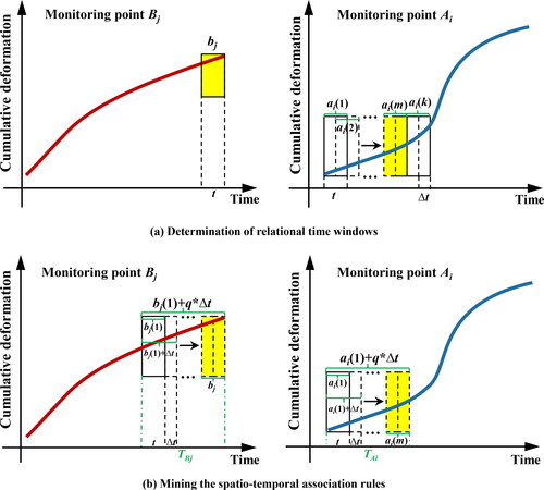
3.2.2. Mining the spatio-temporal association rules

As shown in Figure 1(b), the relational time windows $b_j$ and $a_i(m)$ for monitoring points $B_j$ and $A_i$ were obtained. The time series from the starting time at monitoring point $A_i$ to the ending time of the relational time window $a_i(m)$ constitutes $T_{A_i}.$ The time series $T_{B_j}$ starts at the fixed time window $b_j$ of monitoring point $B_j$ and goes to the time point at which it contains the same amount of data as in $T_{A_i}.$ There may be a spatio-temporal association between time series $T_{A_i}$ and $T_{B_j};$ monitoring point $B_j$ may trend towards the EDZ according to the deformation trend of $A_i.$ The ARM method combined with GRA can be used to mine the spatio-temporal association rules between the time series as determined by the relational time windows. The procedure is as follows:

1. The total number of time windows is determined. The time series $T_{B_j}$ and $T_{A_i}$ that may exist spatio-temporal association were obtained, and the total number of sliding time windows in time series $T_{A_i}$ was determined to be m. As shown in Figure 1(b), the time windows $b_j(1)$ and $a_i(1)$ are composed of the earliest t data in the time series $T_{B_j}$ and $T_{A_i}$^, respectively. Time window $a_i(1)$ is equivalent to the first sliding time window . The time series in time windows $b_j(1)$ and $a_i(1)$ are extended simultaneously until the end of time series $T_{B_j}$ and $T_{A_i}.$ The length of each time series extension is Δt, which equals the time series length of each slide. The two time series $T_{B_j}$ and $T_{A_i}$ are of equal length. Therefore, the total number of time windows formed in the extension of the time series is the same as the total number of sliding time windows, i.e. m.

2. The minimum support $S_{\min }$ is set. The GRG between the two time windows formed by each extension in time series $T_{B_j}$ and $T_{A_i}$ is calculated. The threshold of GRG is also set. The ratio of the number of time windows that meet the GRG threshold to the total number of time windows is defined as the support. The ratio must not be lower than $S_{\min }.$ The total number of time windows has been determined to be m, so the number of time windows that do not meet the GRG threshold cannot exceed $m\ast (1-S_{\min })$ in the process of extending the time series.

3. The calculation process is conducted according to the minimum support $S_{\min }.$ As shown in Figure 1(b), the GRG is calculated for the first time window, $b_j(1)$ and $a_i(1).$ By extension of the time series, the GRG is calculated for the second time window, $b_j(1)+\Delta t$ and $a_i(1)+\Delta t.$ When the GRG $R(b_j(1)+q\ast \Delta t,a_i(1)+q\ast \Delta t)$ $(q=0,1,\dots ,m-1)$ of the (q + 1) time window is obtained, the cumulative count of time windows that are lower than the GRG threshold exceeds $m\ast (1-S_{\min }).$ At this time, the calculation process between monitoring points $B_j$ and $A_i$ is terminated, and monitoring point $A_i$ is eliminated. This calculation process is continued between monitoring point $B_j$ and the other monitoring points in the EDZ. Monitoring points that do not meet the minimum support are eliminated. The retained monitoring points meet the minimum support requirements until the ending time of the time series as-determined by the relational time windows.

4. The minimum confidence is set. In the time series data that meet the minimum support, the GRG $R(b_j(1)+q\ast \Delta t,a_i(1)+q\ast \Delta t)$ of the (q + 1) time window and the GRG $R(b_j(1)+(q-1)\ast \Delta t,a_i(1)+(q-1)\ast \Delta t)$ of the q time window were obtained in Step (III). To reflect the sustainability of similar deformation trends over time, the ratio of the GRG of the (q + 1) time window to the GRG of the q time window is defined as the confidence.

If the above calculation process reveals that time series $T_{B_j}$ of monitoring point $B_j$ and time series $T_{A_i}$ of monitoring point $A_i$ in the adjacent HDZ and EDZ meet the requirements of the minimum support and minimum confidence, we can conclude that there is a spatio-temporal association between time series $T_{B_j}$ and $T_{A_i}.$

3.3. Surface deformation prediction

The modelling process is as follows (with monitoring points $B_j$ in the HDZ and $A_i$ in the EDZ as examples):

1. There is spatio-temporal association between time series $T_{B_j}$ and $T_{A_i}.$ $T_{B_j}$ is the time series of monitoring point $B_j$ in the HDZ. $T_{A_i}$ is the time series of monitoring point $A_i$ in the adjacent EDZ. The time series data $T_{A_i}$ are input as a training sample set, and the time series data $T_{B_j}$ are used as the output. This allows the SVR model to learn the spatio-temporal association rules between the two time series data.

2. After the SVR model establishes the spatio-temporal relationship between the two time series $T_{B_j}$ and $T_{A_i}$ in the form of a function, the subsequent data from monitoring point $A_i$ can be used as an input to predict the deformation value at monitoring point $B_j$ based on the spatio-temporal association.

Surface deformation zones expand and evolve over time. The deformation zones that develop slowly (HDZ) eventually evolve into adjacent, more-developed deformation zones (EDZ). These monitoring points may deviate from the deformation development tendency in the HDZ and evolve according to the deformation characteristics of the adjacent EDZ, marking the appearance of catastrophic deformation. The spatio-temporal association rules can reveal the spatio-temporal evolution law between adjacent HDZ and EDZ zones. It can find out that monitoring point $B_j$ in HDZ has begun to develop to the EDZ and monitoring point $A_i$ in EDZ owns its current and future deformation trend. Therefore, the SVR prediction model based on spatio-temporal associations between monitored HDZ and EDZ data can predict the catastrophic deformation at the monitoring points in the HDZ as it is evolving into the adjacent EDZ.

4. Application

4.1. General situation of Chengchao iron mine

Previous researchers have introduced the distribution of rock masses, geological structure, in situ stress field, hydrogeological conditions, mining method, surface deformation, rock strata movement, and other basic information regarding Chengchao iron mine, China (Cheng et al. 2018, 2017; Deng et al. 2018; Song et al. 2018; Xia et al. 2019). We will not repeat this information here instead focus on the information closely related to this article. The non-pillar sublevel caving method is adopted to allow overburden of the ore body to move, which inevitably leads to surface deformation. The scope of this deformation continuously expands as the depth and range of underground mining expand. As of October 2012, the length (along the NWW direction) of the deformation zone caused by the mining area was more than 3 km and the width more than 1.5 km in Chengchao. Across this large deformation zone (apart from the collapse zone), 201 monitoring points were arranged for GPS static survey. Since 2006, these monitoring points have been measured once monthly to gather mining-induced surface deformation data.

The surface deformation area can be divided into four zones based on previously published information. First is a fracture extension zone which has a folding deformation curve and substantial cumulative deformation. The fracture closure zone has S-shaped curve and large cumulative deformation. The fracture formation zone is defined by the straight-line curve and the cumulative deformation is medium. Finally, the deformation curve of the deformation accumulation zone fluctuates and its cumulative deformation is small (Cheng et al. 2017).

4.2. Surface deformation zoning

To validate the proposed method at the lowest possible computation load, 22 monitoring points of surface deformation near the excavation are selected as testing samples. These points are divided into four clusters (k= 4) based on the strata movement mechanism around the collapse zone and the previously determined division of rock mass deformation. The DTW algorithm is applied to measure the distances between time series of surface deformation with Equations (1)(1) $$\mathit{DTW}\left(A,B\right)=\underset{W=\left\{w_1,w_2,\dots ,w_K\right\}}{\min }\left\{\sqrt{\sum _{k=1,w_k=\left(i,j\right)}^K{\left(a_i-b_j\right)}^2}\right\}$$(1) and (2)(2) $$\Gamma \left(i,j\right)=\{\begin{array}{c}\sum _{k=1}^j{D}_{ik},\begin{array}{cc}\begin{array}{ccc}\begin{array}{ccc}& & \end{array}& \begin{array}{cc}& \end{array}& \end{array}& \end{array}\text{if}\begin{array}{cc}& i=1,\begin{array}{cc}& j\in \left[1:m\right]\end{array}\end{array}\\ \sum _{k=1}^i{D}_{kj},\begin{array}{cc}\begin{array}{ccc}\begin{array}{ccc}& & \begin{array}{cc}& \end{array}\end{array}& & \end{array}& \end{array}\text{if}\begin{array}{cc}& j=1,\begin{array}{cc}& i\in \left[1:n\right]\end{array}\end{array}\\ D_{ij}+\min \left\{\Gamma \left(i,j-1\right),\Gamma \left(i-1,j\right),\Gamma \left(i-1,j-1\right)\right\},\begin{array}{cc}& \text{else}.\end{array}\end{array}$$(2) . By minimizing the objective function specified in Equation (3)(3) $$\text{Minimize}:d={{\sum }_{j=1}^k{\sum }_{i=1}^n\Vert x_{ij}-c_j\Vert }^2$$(3) , the improved k-means algorithm assigns cluster k to 22 monitoring points.

The clustering results in Figure 2(a) show that monitoring points E04, E05, and LG2 fall into the same cluster; their deformation curves show a folding-line trend which is consistent with fracture extension zone characteristics. Monitoring points F02, F04, F05, F06, F07, E01, and E03 follow an S-shaped curve consistent with the fracture closure zone. Monitoring points D01, D02, LC42, E09, D09, C05, C08, and E11 follow a straight line which conforms to the fracture formation zone. Monitoring points C03, C04, C09, and D12 are in the same cluster and fluctuate, forming the deformation accumulation zone. The surface deformation zones in Figure 2(b) are delineated based on these observations listed in Table 1.

Figure 2. The results of monitoring point clustering and surface deformation zoning: (a) The deformation curves of four clusters of monitoring points; (b) Four surface deformation zones in the horizontal displacement contour map (Cheng et al. 2017).

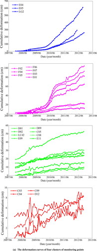
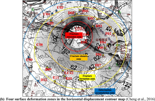
Table 1. Monitoring point clusters and surface deformation zones.

Clustering results	Monitoring points	Cumulative deformation	Curve type	Deformation zones	Location
Cluster one	E04, E05, LG2	Very large	Folding curve	Fracture extension zone	Close to the deformation centre
Cluster two	F02, F04, F05, F06, F07, E01, E03	Large	S-shaped curve	Fracture closure zone	Close to the fracture extension zone
Cluster three	D01, D02, LC42, E09, D09, C05, C08, E11	Medium	Straight line	Fracture formation zone	Close to the fracture closure zone
Cluster four	C03, C04, C09, D12	Small	Fluctuation curve	Deformation accumulation zone	Close to the fracture formation zone

The clustering of the monitoring points and the division of deformation zones creates a sound basis for the spatio-temporal associaiton rule mining between the fracture formation zone (i.e. the HDZ) and fracture closure zone (i.e. the EDZ) to predict the deformation of monitoring points in fracture formation zone. This work is also the basis for the spatio-temporal associaiton rule mining between the fracture extension zone (i.e. the EDZ) and fracture closure zone (i.e. the HDZ) to predict the deformation of monitoring points in fracture closure zone.

4.3. Spatio-temporal association rules mining

To effectively determine similarities and associations of deformation trends between the monitoring points in adjacent deformation zones, the cumulative deformation values at all monitoring points are transformed into the deformation rate. According to the total amount of data for each monitoring point, the minimum measurement unit to determine the similarities and associations of the deformation data is the time window that contains the deformation data for an 8-month period. The time series length for each sliding of time window and each expansion of time series is set to 2 months. The calculation is operated in the following stepwise process.

4.3.1. Determining relational time windows by GRA

The last 8-month time series data (March–October 2012) of the monitoring points in the fracture formation zone form the fixed time window. The earliest 8-month time series data (from December 2007 to July 2008) of the monitoring points in the fracture closure zone constitute the first sliding time window. To obtain all sliding time windows, the first time window slides backward 2 months each time. The sliding time windows traverse all the deformation data before the turning point (January 2010) of the deformation trend of the monitoring points in the fracture closure zone. The GRG between the fixed time window and all sliding time windows are calculated.

The sliding time window owning the longest sliding time period, which the GRG is more than 0.85 and the sliding time period is longer than $5\ast \Delta t,$ is specified here as the relational time window for the fixed time window. The monitoring data from December 2007 to January 2010 include 10 sliding time windows with a sliding time period of $9\ast \Delta t.$ The minimum standard of the sliding time period is not less than $5\ast \Delta t$ under the requirement of 1/2 multiple. It is a minimum standard for the length of the time series with spatio-temporal association to ensure accurate predictions. This 0.85 is the GRG threshold when the relational time windows are to be determined. In cases like this, too high a threshold can obscure the relational time windows; in reality, there are no relational time windows with very consistent deformation trends. Too low a threshold, conversely, creates varying deformation trends across the relational time windows and may render inaccurate ARM and prediction. The GRG threshold of 0.85 is finally selected by trial-and-error.

In Table 2, the GRG calculation results between the fixed time window of monitoring point D01 in the fracture formation zone and the sliding time windows of all the monitoring points in the fracture closure zone are listed as an example. The GRG results between the fixed time window of monitoring point D01 and the sliding time windows of monitoring points F02, E03, F04, F05, and F06 show that the longest sliding time period of the sliding time windows that meet the threshold of 0.85 is shorter than $5\ast \Delta t.$ There may be spatio-temporal association in this case, but the time period is too short, so these monitoring points are eliminated. In the GRG between monitoring points D01 and E01, F07, the longest sliding time period of the sliding time window that meets the threshold of 0.85 is longer than $5\ast \Delta t;$ thus, the sliding time window from June 2009 to January 2010 of monitoring points E01 and F07 can be considered the relational time window of the fixed time window from March 2012 to October 2012 of monitoring point D01. The relational time windows between the fracture formation and fracture closure zones were obtained according to the same principle as listed in Table 3.

Table 2. GRG between fixed time window of monitoring point D01 and sliding time windows of all the monitoring points in the fracture closure zone.

Time period (year/month)	RD01-E01	RD01-F02	RD01-E03	RD01-F04	RD01-F05	RD01-F06	RD01-F07
2007/12–2008/07	0.9276	0.8760	0.8459	0.9021	0.8691	0.8589	0.8040
2008/02–2008/09	0.8045	0.7950	0.8215	0.8582	0.8383	0.8325	0.8400
2008/04–2008/11	0.7129	0.7338	0.7913	0.8257	0.7620	0.8324	0.8018
2008/06–2009/01	0.6378	0.6163	0.7433	0.8553	0.8303	0.8757	0.8238
2008/08–2009/03	0.5848	0.5649	0.7092	0.7850	0.7603	0.8245	0.7915
2008/10–2009/05	0.6283	0.5573	0.7503	0.7691	0.7360	0.8126	0.7982
2008/12–2009/07	0.6953	0.6035	0.7526	0.7767	0.7151	0.7857	0.7825
2009/02–2009/09	0.7674	0.7334	0.7567	0.7604	0.6579	0.8251	0.8164
2009/04–2009/11	0.8166	0.7807	0.7349	0.7816	0.6714	0.7591	0.8377
2009/06–2010/01	0.8582	0.7993	0.7798	0.8178	0.6517	0.7596	0.8592

Note: Bolded numbers represent relational time windows.

Table 3. GRG between fixed time windows of monitoring points in fracture formation zone and sliding time windows of monitoring points in fracture closure zone.

Time period (year/month)	RD01-E01	RD01-F07	RD02-E01	RLC42-E01	RLC42-F02	RC05-F07	RC08-E01	RC08-F07	RD09-E03	RE09-E01	RE09-F02	RE09-F07	RE11-E01
2007/12–2008/07	0.9276	0.8040	0.8961	0.8702	0.8475	0.7781	0.8269	0.9371	0.8583	0.8592	0.8376	0.8460	0.8441
2008/02–2008/09	0.8045	0.8400	0.8397	0.7949	0.8379	0.8442	0.8233	0.8176	0.8144	0.7982	0.8215	0.7853	0.7888
2008/04–2008/11	0.7129	0.8018	0.7668	0.7212	0.7428	0.7877	0.7860	0.8464	0.8352	0.7287	0.7460	0.8636	0.7302
2008/06–2009/01	0.6378	0.8238	0.6756	0.6369	0.6251	0.8314	0.6884	0.8567	0.7044	0.6301	0.6136	0.8741	0.6702
2008/08–2009/03	0.5848	0.7915	0.5803	0.6292	0.5945	0.7979	0.6382	0.8496	0.7239	0.6193	0.6034	0.8235	0.6364
2008/10–2009/05	0.6283	0.7982	0.6199	0.6342	0.5859	0.8351	0.5765	0.9101	0.6209	0.6415	0.5662	0.8370	0.6310
2008/12–2009/07	0.6953	0.7825	0.7023	0.7434	0.6370	0.8359	0.7113	0.8985	0.7585	0.7718	0.6640	0.8107	0.7128
2009/02–2009/09	0.7674	0.8164	0.7671	0.7875	0.7787	0.9041	0.8280	0.8353	0.8356	0.7694	0.7695	0.8304	0.7601
2009/04–2009/11	0.8166	0.8377	0.8732	0.8265	0.7867	0.8638	0.8235	0.8589	0.8612	0.8122	0.7780	0.9155	0.8144
2009/06–2010/01	0.8582	0.8592		0.9197	0.8794		0.8756	0.8573		0.8973	0.8597	0.8614	0.8775

Note: Bolded numbers represent relational time windows.

4.3.2. Mining the spatio-temporal association rules

We determined which sliding time window of the fracture closure zone had a deformation trend most similar to that of the fixed time window of the fracture formation zone to secure proper relational time windows. The time series in the fracture closure zone from the starting time of monitoring points to the ending time of the relational time window are likely to have spatio-temporal association with the time series in the fracture formation zone of the same length before the ending time of the fixed time window. To mine the association rules, we applied the ARM method combined with GRA.

1. The total number of time windows was determined. The time series that may have spatio-temporal association were identified based on the relational time windows given in Table 3. There may be spatio-temporal association between the time series from December 2007 to January 2010 of monitoring points E01, F07, and F02 in the fracture closure zone and the time series from September 2010 to October 2012 of monitoring points D01, LC42, C08, E09, and E11 in the fracture formation zone. Similarly, there may be spatio-temporal association between the time series from December 2007 to November 2009 of monitoring points E01, F07, and E03 in the fracture closure zone and the time series from November 2010 to October 2012 of monitoring points D02, C05, and D09 in the fracture formation zone. As listed in Table 3, a maximum of 10 time windows formed at the monitoring points in the fracture closure zone.

2. The minimum support was set. In the time windows formed by extension of the time series, the ratio of the number of time windows that meet the GRG threshold of 0.7 to the total number of time windows was not less than 60% in this case. The GRG threshold of 0.7 and the minimum support of 60% were determined by trial-and-error (similarly to the above GRG threshold of 0.85, we tested various GRG thresholds from 0.5 to 1 (Zhang, Wu, Chen, Dai, et al. 2020) to determine which one was optimal in terms of final prediction effects. The minimum support was determined similarly by the final prediction accuracy). The total number of time windows is at most 10; thus, the number of time windows that do not meet the GRG threshold cannot exceed 4.

3. The calculation process was conducted according to the minimum support. Monitoring point LC42 in the fracture formation zone is discussed here as an example. By extension of the time series, several new time windows formed on the basis of the time window (B8) from September 2010 to April 2011 of monitoring point LC42 and the time window (A8) from December 2007 to July 2008 of monitoring points E01 and F02 in the fracture closure zone are listed as R_LC42-E01 and R_LC42-F02 in Table 4. When the GRG s of the sixth time window (A8 + 10-B8 + 10) between monitoring points E01 and LC42 were calculated, the number of time windows with a GRG lower than 0.7 exceeded 4. The calculation process was terminated and monitoring point E01 was eliminated. This process continued between LC42 and F02, the GRG met the minimum support until the ending time of the relational time windows. Then the monitoring points LC42 and F02 were retained.

   The GRG s of R_D01-E01 and R_D01-F07 both met the minimum support requirements. The monitoring points with higher GRG were retained under this condition. In the time series determined by the relational time windows between the fracture formation zone and fracture closure zone, the time series of the monitoring points D01-E01, D02-E01, LC42-F02, C05-F07, C08-E01, D09-E03, and E09-F02 that met the minimum support requirement were further obtained in Table 4.

4. The minimum confidence was set. In the monitoring points and corresponding time series of the fracture formation and fracture closure zones that reach the requirement of the minimum support as shown in Table 4, the ratio of the GRG of the latter time window to the GRG of the former time window is more than 0.9 (i.e. the minimum confidence) (Zhao 2018); the minimum confidence requirement is met in this case.

Table 4. GRG calculation results in the process of extension of time series.

Time windows	RD01-E01	RD01-F07	RD02-E01	RLC42-E01	RLC42-F02	RC05-F07	RC08-E01	RC08-F07	RD09-E03	RE09-E01	RE09-F02	RE09-F07	RE11-E01
A8-B8	0.6907	0.7053	0.7722	0.6411	0.6713	0.6588	0.7673	0.7216	0.6759	0.6761	0.7664	0.6633	0.7215
A8 + 2-B8 + 2	0.6606	0.7127	0.7713	0.6546	0.6709	0.6785	0.7201	0.7052	0.7269	0.6443	0.7303	0.6422	0.6969
A8 + 4-B8 + 4	0.7667	0.6976	0.8402	0.7280	0.6869	0.7206	0.7829	0.6736	0.8013	0.7130	0.7539	0.6346	0.7085
A8 + 6-B8 + 6	0.7388	0.6997	0.7913	0.6864	0.7173	0.7329	0.7457	0.6844	0.7586	0.6785	0.7322	0.6643	0.6797
A8 + 8-B8 + 8	0.7178	0.7062	0.7639	0.6589	0.7265	0.7400	0.7238	0.6771	0.7443	0.6573	0.7524	0.6659	0.6741
A8 + 10-B8 + 10	0.7073	0.7112	0.7328	0.6875	0.7205	0.7438	0.7375	0.6951	0.7672	0.6864	0.7468		0.6133
A8 + 12-B8 + 12	0.7189	0.7127	0.7379		0.7378	0.7547	0.6905	0.6893	0.7809		0.7603		0.6379
A8 + 14-B8 + 14	0.7104	0.7068	0.7378		0.7554	0.7274	0.7016		0.7641		0.7781
A8 + 16-B8 + 16	0.7218	0.7039	0.7581		0.7596	0.7228	0.7214		0.7693		0.7814
A8 + 18-B8 + 18	0.7303	0.7023			0.7632		0.7152				0.7747

Note: Bolded numbers represent monitoring points that do not meet the minimum support requirement and are eliminated.

The calculation of the GRG between the fixed time windows and sliding time windows of the monitoring points in adjacent zones determines relational time windows with similar deformation trends. Table 3 shows where relational time windows were found between the fracture closure zone and fracture formation zone; the time series with possible spatio-temporal association among the corresponding monitoring points was determined accordingly.

The extension of the time series was performed on the time series with a possible spatio-temporal association, and the time windows formed in the process should meet the minimum support and minimum confidence requirements. The calculation results shown in Table 4 indicate that the minimum support and minimum confidence requirements were met in this case (except bolded numbers), so strong association rules were generated accordingly. There is spatio-temporal association between the time series from September 2010 to October 2012 of monitoring points D01, LC42, C08, and E09 in the fracture formation zone and the time series from December 2007 to January 2010 of monitoring points E01, F02, E01, and F02 in the fracture closure zone. Similarly, there is spatio-temporal association between the time series from November 2010 to October 2012 of monitoring points D02, C05, and D09 in the fracture formation zone and the time series from December 2007 to November 2009 of monitoring points E01, F07, and E03 in the fracture closure zone. The number of time windows is more than 4 when the grey correlation degree between monitoring points E11 and E01 is less than 0.7. The deformation trends of monitoring points E11 and E01 differ markedly. The E11 does not show the characteristics of fracture closure zone and may follow its original deformation trend.

The ARM method was similarly applied to the fracture closure zone and fracture extension zone. Surface deformation in the deformation accumulation zone is very small, so a slight deviation in the monitoring process has a great impact on the deformation value. Even if the deformation accumulation zone evolves into the fracture formation zone, the risk to the infrastructure’s safety in this case is relatively small, so we did not target this zone for analysis.

The time series with spatio-temporal association among the corresponding monitoring points between adjacent zones of the fracture formation zone, fracture closure zone, and fracture extension zone are listed in Table 5. We found spatio-temporal association between the monitoring points F02, E03, and F07 in fracture closure zone and the monitoring points in the fracture extension zone. Other monitoring points in the fracture closure zone did not show spatio-temporal association with the monitoring points in fracture extension zone. The cumulative deformation of these monitoring points would continue to develop in accordance with their original deformation.

Table 5. Spatio-temporal association for time series data of monitoring points in adjacent zones.

HDZs	Monitoring points in HDZs	The time period of monitoring points in HDZs with association	The time period of monitoring points in EDZs with association	Monitoring points in EDZs	EDZs
Fracture formation zone	D01	2010/09–2012/10	2007/12–2010/01	E01	Fracture closure zone
	D02	2010/11–2012/10	2007/12–2009/11	E01
	LC42	2010/09–2012/10	2007/12–2010/01	F02
	C05	2010/11–2012/10	2007/12–2009/11	F07
	C08	2010/09–2012/10	2007/12–2010/01	E01
	D09	2010/11–2012/10	2007/12–2009/11	E03
	E09	2010/09–2012/10	2007/12–2010/01	F02
Fracture closure zone	F02	2011/01–2012/10	2007/12–2009/09	E04	Fracture extension zone
	E03	2011/03–2012/10	2007/12–2009/07	E04
	F07	2010/11–2012/10	2007/12–2009/11	LG2

We focused our subsequent analysis on the fracture formation zone and the zone in which monitoring points F02, E03, and F07 are located. The future deformation of monitoring points F02, E03, and F07, especially in regards to catastrophic deformation, should be accurately predicted to prevent major damage from infrastructure collapse (similar to the damage of the fracture extension zone). In the fracture formation zone, apart from monitoring point E11, the remaining seven monitoring points show fracture closure zone characteristics. Thus, it is necessary to accurately predict the surface deformation of the fracture formation zone, especially the catastrophic deformation, in order to fully prevent the uneven deformation and collapse of infrastructure (similar to the damage of the fracture closure zone).

4.4. Surface deformation prediction

SVR was applied to build the prediction model. The radial basis function was used as the kernel function of SVR and the grid-search method was used to select the C and g parameters for SVR in this study. In Table 5, the time series data from the monitoring points in the fracture closure zone were used as the training sample input data, and the time series data from the monitoring points in the fracture formation zone were used as the expected output data. The SVR model was built based on the spatio-temporal association between the fracture closure zone and the fracture formation zone. The deformation data from February 2010 to September 2010 and from December 2009 to July 2010 for the corresponding monitoring points in the fracture closure zone were used as input for the testing samples to predict the deformation value in the following 8 months (from November 2012 to June 2013) of the fracture formation zone. The same procedure was followed to predict deformation in the fracture closure zone according to the corresponding time series with spatio-temporal association between the fracture extension zone and fracture closure zone (Table 5). Therefore, in the established prediction model, 71 − 76% of samples are used for training, and the remaining samples are used for testing. This delineation meets the requirements of 2/3 − 4/5 samples as training samples mentioned by Zhou (2016). The prediction results of the SVR model based on spatio-temporal association for the fracture formation zone and fracture closure zone are shown in Figures 3 and 4.

Figure 3. Fracture formation zone prediction results.

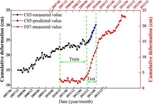
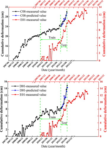
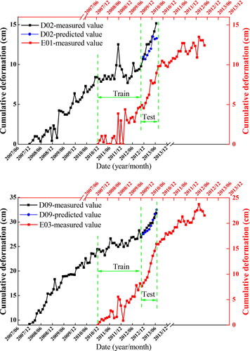
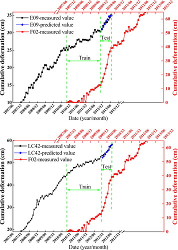
Figure 4. Fracture closure zone prediction results.

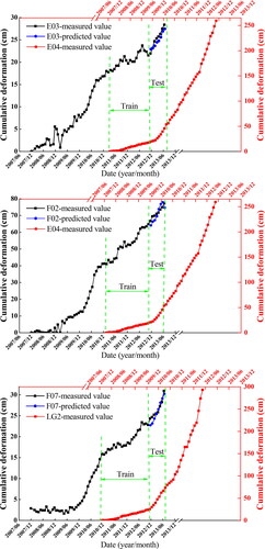
The prediction results of the monitoring points with spatio-temporal association are shown in Figures 3 and 4. There is a general consistency between the deformation trends (i.e. deformation rate) of the monitoring points with spatio-temporal association. The deformation trend from November 2010 to June 2013 for monitoring point C05 is generally consistent with the deformation trend from December 2007 to July 2010 for monitoring point F07. The SVR model learns the spatio-temporal association rules between the training samples to finish prediction in the testing samples. The testing samples (e.g. the accelerating deformation from December 2009 to July 2010 of F07) properly guided the SVR model in predicting the catastrophic deformation (e.g. the accelerating deformation from November 2012 to June 2013 of C05) as per any rapid transformation from gentle to severe or from slow to rapidly accelerating deformation.

5. Discussion

5.1. Comparison of prediction accuracy for different models

Li et al. (2011) and Chen and Deng (2014) introduced the time series prediction (TSP ) model based on SVR. The key to TSP is the reconstruction of data to transform a one-dimensional time series into a matrix form to obtain the correlation between time series datasets. The TSP model based on SVR is established based on the correlation. To illustrate the advantages of the proposed STARM model, we compared it against the TSP model.

To make the reconstructed data fully reflect the characteristics of the system, the appropriate selection of the embedding dimension is key for TSP. The embedding dimension denotes the number of observations that impact the prediction of the next series. The criterion of final prediction error introduced by Li et al. (2011) and Chen and Deng (2014) is used to determine the best embedding dimension. By calculation, a minimum final prediction error is obtained when the embedding dimension is 4. Because the time series of surface deformation is short, the step size of prediction is chosen as one, according to the research of Chen and Deng (2014).

The surface deformation data from November 2012 to June 2013 are selected as the testing sample similar to that of the STARM model , and the rest of the data are used as the training sample. Then, the rolling prediction method applied by Li et al. (2011) and Chen and Deng (2014) is used for the reconstruction data. It is a one-step prediction first, and then the output is fed back to the input to predict the value at a certain time in the future. The prediction errors of the STARM and TSP models were compared as per mean absolute percentage error (MAPE), mean absolute error (MAE), and root mean square error (RMSE).

Table 6 presents the MAPE, MAE, and RMSE evaluation criteria results. Except that the prediction accuracy of the TSP model for the monitoring points C08 and LC42 is slightly higher than that of the STARM model , the prediction effect of the STARM model is all better than that of the TSP model for other monitoring points. It can be said that the prediction considering spatio-temporal associations is superior to the TSP for surface deformation. The deformation trends predicted by the STARM model are generally consistent with those actual sharp changes, as shown in Figures 3 and 4. The prediction results of the TSP model are lower than the real values for most monitoring points, as shown in Figure 5. Therefore, it can be concluded that the STARM model is effective and accurate to predict the surface deformation, especially the catastrophic deformation.

Figure 5. Prediction results by TSP model.

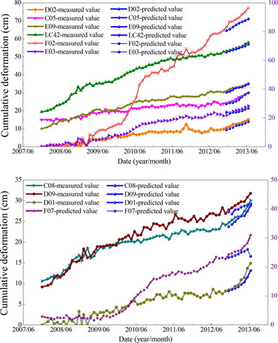
Table 6. Comparison of prediction error between the TSP and STARM models.

Models	Performance indicators	D01	D02	C05	C08	D09	E09	LC42	F02	F07	E03
TSP model	MAPE (%)	11.30	9.43	2.10	2.00	2.78	1.66	1.01	5.27	7.40	5.13
	MAE	1.29	1.19	0.55	0.54	0.84	0.54	0.56	3.83	2.08	1.30
	RMSE	1.43	1.23	0.70	0.57	0.99	0.66	0.63	4.01	2.88	1.38
STARM model	MAPE (%)	5.13	6.44	0.68	2.23	1.94	1.36	1.06	3.63	3.51	3.02
	MAE	0.54	0.85	0.18	0.59	0.58	0.45	0.59	2.61	0.91	0.77
	RMSE	0.84	1.01	0.20	0.64	0.61	0.52	0.71	2.67	1.01	0.82

5.2. Analysis of prediction accuracy for different monitoring points

A comparative analysis of the prediction accuracy at different monitoring points shows that the surface deformation values predicted by the STARM model for monitoring points C05, C08, D09, E09, and LC42 match the measured values very closely; the MAPEs, MAEs, and RMSEs are within 3%, 0.6 and 0.7 cm, respectively. The prediction accuracy for monitoring points D01, D02, F07, and E03 is moderate, with MAEs and RMSEs lower than 1.1 cm. The prediction accuracy for monitoring point F02 is the lowest; although its MAPE is lower than that of monitoring points D01 and D02, the MAE and RMSE are both higher, reaching more than 2 cm. The prediction accuracy could be improved if the monitoring data from 201 GPS static survey points at the Chengchao iron mine are used for spatio-temporal association rule mining and prediction.

5.3. Physical meaning of spatial association

During the process of surface deformation, the cumulative deformation over time at monitoring points on a rock mass in the same state (e.g. elastic, plastic, and fracture) presents a consistent trend, and the magnitude varies slightly. The cumulative deformation over time at monitoring points on a rock mass in different states shows different trends and greatly disparate deformation values. As the state of a rock mass changes (e.g. from elastic to plastic or from plastic to fracture), the cumulative deformation of its monitoring points departs from what would be expected based on the historical deformation trend.

The surface deformation monitoring area in cases such as the one described here is often not very large. The regional geological conditions and mechanical parameters may also be very similar, so the cumulative deformation of the surface deformation as it changes state can be used as a reference for catastrophic deformation prediction. For example, the deformation characteristics of a plastic rock mass are useful information for predicting deformation in an elastic rock mass during state transformation. This is evidence of the physical meaning of the spatial association of surface deformation.

5.4. Deficiencies of the STARM model

Although the STARM model considers sufficiently the spatio-temporal association of surface deformation and has a good prediction performance, there are two aspects to be further improved. First, considering the deficiencies of the grid-search method, some optimization algorithms can be considered for selecting the optimal hyperparameters of the SVR model (Bergstra and Bengio 2012; Rusek 2020;); second, recurring to the advantage of the Bayesian networks or fuzzy systems (Rusek and Wodyński 2010; Rusek et al. 2021), some advanced machine learning methods can also be integrated into the prediction model based on spatio-temporal association.

6. Conclusion

This study proposes a prediction model for surface deformation caused by underground excavation based on spatio-temporal associations. The prediction model is operated in three steps: surface deformation zoning, spatio-temporal association rule mining, and surface deformation prediction. Surface deformation monitoring data are taken at Chengchao Iron Mine, China, as a case study to verify the proposed prediction model. Its prediction results are compared with those of the traditional TSP model. The following conclusions can be drawn.

1. Surface deformation caused by underground mining contains multiple stages or states. The k-means algorithm improved by DTW algorithm is reliable for identifying the EDZ and HDZ, which represent different deformation stages or states. The ARM method combined with the GRA is a feasible tool to mine spatio-temporal association rules between the EDZ and HDZ. Predictions based on spatio-temporal associations are accurate, especially for catastrophic deformation.

2. The spatio-temporal relationship between surface deformation monitoring data is used to establish the prediction model. Therefore, it is unnecessary to collect the data of the variables affecting surface deformation. The spatio-temporal association rules are mined between the EDZ and the HDZ. The prediction errors in the traditional model due to the surface deformation state transition (from the HDZ to the adjacent EDZ) can be alleviated in the proposed STARM model .

3. In the practical case at the Chengchao iron mine, China, the surface deformation that occurs due to underground mining is predicted by the STARM model. The results show that the predicted value is in good agreement with the measured data. Comparing the prediction results with those of the traditional TSP model, the deformation trend predicted by the STARM model is found to be more consistent with the actual sharp changes in catastrophic deformation than that predicted by the time series prediction model; the STARM model is better for the catastrophic deformation predictions.

Abbreviations
AI	=	artificial intelligence
ARM	=	association rule mining
CNNs	=	convolutional neural networks
DTW	=	dynamic time warping
EDZ	=	excessive deformation zone
GPS	=	global position system
GRA	=	grey relation analysis
GRG	=	grey relational grade
HDZ	=	hysteretic deformation zone
InSAR	=	interferometric synthetic aperture radar
LSTM	=	long short-term memory
MAE	=	mean absolute error
MAPE	=	mean absolute percentage error
RMSE	=	root mean square error
STARM	=	Prediction based on spatio-temporal association rule mining
SVR	=	support vector regression
TSP	=	time series prediction

Disclosure statement

No potential conflict of interest was reported by the authors.

Data availability statement

Participants of this study did not agree for the data to be shared publicly, so supporting data is not available.

Additional information

Funding

This article was funded by the National Science Foundation of China (Grant Nos. 51909032, 51874069, and U1903216) and the Fundamental Research Funds for the Central Universities of China (Grant Nos. N180101028 and N180115009).

References

- Ai Y, Li Z, Gan M, Zhang Y, Yu D, Chen W, Ju Y. 2019. A deep learning approach on short-term spatiotemporal distribution forecasting of dockless bike-sharing system. Neural Comput Appl. 31(5):1665–1677.
- Berndt DJ, Clifford J. 1994. Using dynamic time warping to find patterns in time series. KDD Workshop. 10(16):359–370.
- Chai S, Xu Z, Jia Y, Wong WK. 2020. A robust spatiotemporal forecasting framework for photovoltaic generation. IEEE Trans Smart Grid. 11(6):5370–5382.
- Bergstra J, Bengio Y. 2012. Random search for hyper-parameter optimization. J Mach Learn Res. 13:281–305.
- Chen BQ, Deng KZ. 2014. Integration of D-InSAR technology and PSO-SVR algorithm for time series monitoring and dynamic prediction of coal mining subsidence. Surv Rev. 46(339):392–400.
- Chen RP, Zhang P, Kang X, Zhong ZQ, Liu Y, Wu HN. 2019. Prediction of maximum surface settlement caused by earth pressure balance (EPB) shield tunneling with ANN methods. Soils Found. 59(2):284–295.
- Chen R, Zhang P, Wu H, Wang Z, Zhong Z. 2019. Prediction of shield tunneling-induced ground settlement using machine learning techniques. Front Struct Civ Eng. 13(6):1363–1378.
- Cheng G, Chen C, Li L, Zhu W, Yang T, Dai F, Ren B. 2018. Numerical modelling of strata movement at footwall induced by underground mining. Int J Rock Mech Min. 108:142–156.
- Cheng G, Chen C, Ma T, Liu H, Tang C. 2017. A case study on the strata movement mechanism and surface deformation regulation in Chengchao Underground Iron Mine. Rock Mech Rock Eng. 50(4):1011–1032.
- Deng JL. 1982. Control problems of grey systems. Syst Control Lett. 1(5):288–294.
- Deng Y, Chen C, Xia K, Yang K, Sun C, Zheng X. 2018. Investigation on the characteristics of overlying strata caving in the Chengchao Iron Mine, China. Environ Earth Sci. 77(10):362.
- Ding C, Wang G, Zhang X, Liu Q, Liu X. 2021. A hybrid CNN-LSTM model for predicting PM2.5 in Beijing based on spatiotemporal correlation. Environ Ecol Stat. 28(3):503–522.
- Hajihassani M, Kalatehjari R, Marto A, Mohamad H, Khosrotash M. 2020. 3D prediction of tunneling-induced ground movements based on a hybrid ANN and empirical methods. Eng Comput-Germany. 36(1):251–269.
- Hu M, Li W, Yan K, Ji Z, Hu H. 2019. Modern machine learning techniques for Univariate tunnel settlement forecasting: a comparative study. Math Prob Eng. 2019:1–12.
- Jia H, Luo H, Wang H, Zhao F, Ke Q, Wu M, Zhao Y. 2020. ADST: forecasting metro flow using attention-based deep spatial-temporal networks with multi-task learning. Sensors (Basel). 20(16):4574.
- Kim D, Pham K, Park S, Oh J, Choi H. 2020. Determination of effective parameters on surface settlement during shield TBM. Geomech Eng. 21(2):153–164.
- Li J, Gao F, Lu J, Tao T. 2019. Deformation monitoring and prediction for residential areas in the Panji mining area based on an InSAR time series analysis and the GM-SVR model. Open Geosci. 11(1):738–749.
- Li Y, Shuai B. 2020. Origin and destination forecasting on dockless shared bicycle in a hybrid deep-learning algorithms. Multimed Tools Appl. 79(7–8):5269–5280.
- Li P, Tan Z, Yan L, Deng K. 2011. Time series prediction of mining subsidence based on a. SVM Min Sci Technol. 21(4):557–562.
- Liu L, Wen J, Zheng Z, Su H. 2021. An improved approach for mining association rules in parallel using spark streaming. Int J Circ Theor Appl. 49(4):1028–1039.
- Liu X, Hussein SH, Ghazali KH, Tung TM, Yaseen ZM, Xin B. 2021. Optimized adaptive neuro-fuzzy inference system using metaheuristic algorithms: application of shield tunnelling ground surface settlement prediction. Complexity. 2021:1–15.
- Luo X, Gan W, Wang L, Chen Y, Meng X, Ye X. 2020. A prediction model of structural settlement based on EMD-SVR-WNN. Adv Civ Eng. 2020:1–11.
- Lv Y, Liu T, Ma J, Wei S, Gao C. 2020. Study on settlement prediction model of deep foundation pit in sand and pebble strata based on grey theory and BP neural network. Arab J Geosci. 13(23):1238.
- Macqueen J. 1967. Some methods for classification and analysis of multivariate observations. In: Macqueen J, editor. Proceedings of Berkeley Symposium on Mathematical Statistics & Probability; Sep 11-13; Los Angeles. University of California. p. 281–297.
- Nikakhtar L, Zare S, Nasirabad HM, Ferdosi B. 2020. Application of ANN-PSO algorithm based on FDM numerical modelling for back analysis of EPB TBM tunneling parameters. Eur J Environ Civil Eng. 24:1–18.
- Pak U, Ma J, Ryu U, Ryom K, Juhyok U, Pak K, Pak C. 2020. Deep learning-based PM2.5 prediction considering the spatiotemporal correlations: a case study of Beijing, China. Sci Total Environ. 699:133561.
- Rusek J, Tajduś K, Firek K, Jędrzejczyk A. 2021. Score-based Bayesian belief network structure learning in damage risk modelling of mining areas building development. J Cleaner Prod. 296:126528.
- Rusek J. 2020. The point nuisance method as a decision-support system based on Bayesian inference approach. Arch Min Sci. 65(1):117–127.
- Rusek J, Wodyñski A. 2010. Creating a model of technical wear of buildings in mining areas with the use of Fuzzy inference systems. Geomat Environ Eng. 4:115–123.
- Shaheen M, Shahbaz M, Guergachi A. 2013. Context based positive and negative spatio-temporal association rule mining. Knowledge-Based Syst. 37:261–273.
- Shen D, Zhang L, Cao J, Wang S. 2018. Forecasting citywide traffic congestion based on social media. Wireless Pers Commun. 103(1):1037–1057.
- Son H, Jang Y. 2020. Partial convolutional LSTM for spatiotemporal prediction of incomplete data. IEEE Access. 8:164762–164774.
- Song X, Chen C, Xia K, Yang K, Chen S, Liu X. 2018. Analysis of the surface deformation characteristics and strata movement mechanism in the main shaft area of Chengchao Iron Mine. Environ Earth Sci. 77(9):335.
- Vapnik V. 1995. The nature of statistical learning theory. 2nd ed. New York (NY): Springer-Verlag.
- Wang RT, Ho CTB, Oh K. 2010. Measuring production and marketing efficiency using grey relation analysis and data envelopment analysis. Int J Prod Res. 48(1):183–199.
- Wang X, Yu F, Pedrycz W. 2016. An area-based shape distance measure of time series. Appl Soft Comput. 48:650–659.
- Xia K, Chen C, Zheng Y, Zhang H, Liu X, Deng Y, Yang K. 2019. Engineering geology and ground collapse mechanism in the Chengchao Iron-ore Mine in China. Eng Geol. 249:129–147.
- Xie DF, Wang MH, Zhao XM. 2020. A spatiotemporal apriori approach to capture dynamic associations of regional traffic congestion. IEEE Access. 8:3695–3709.
- Yan K, Dai Y, Xu M, Mo Y. 2019. Tunnel surface settlement forecasting with ensemble learning. Sustainability. 12(1):232.
- Yang G, Wang Y, Yu H, Ren Y, Xie J. 2018. Short-term traffic state prediction based on the spatiotemporal features of critical road sections. Sensors (Basel). 18(7):2287.
- Zang H, Liu L, Sun L, Cheng L, Wei Z, Sun G. 2020. Short-term global horizontal irradiance forecasting based on a hybrid CNN-LSTM model with spatiotemporal correlations. Renew Energy. 160:26–41.
- Zhang F, Zhu X, Hu T, Guo W, Chen C, Liu L. 2016. Urban link travel time prediction based on a gradient boosting method considering spatiotemporal correlations. Int J Geo-Inf. 5(11):201.
- Zhang H, He J, Bao J, Hong Q, Shi X. 2020. A hybrid spatiotemporal deep learning model for short-term metro passenger flow prediction. J Adv Transp. 2020:1–12.
- Zhang K, Lyu HM, Shen SL, Zhou A, Yin ZY. 2020. Evolutionary hybrid neural network approach to predict shield tunneling-induced ground settlements. Tunn Undergr Sp Tech. 106:103594.
- Zhang P. 2019. A novel feature selection method based on global sensitivity analysis with application in machine learning-based prediction model. Appl Soft Comput. 85:105859.
- Zhang P, Li H, Ha QP, Yin ZY, Chen RP. 2020. Reinforcement learning based optimizer for improvement of predicting tunneling-induced ground responses. Adv Eng Inf. 45:101097.
- Zhang P, Wu HN, Chen RP, Chan THT. 2020. Hybrid meta-heuristic and machine learning algorithms for tunneling-induced settlement prediction: a comparative study. Tunn Undergr Sp Technol. 99:103383.
- Zhang P, Wu HN, Chen RP, Dai T, Meng FY, Wang HB. 2020. A critical evaluation of machine learning and deep learning in shield-ground interaction prediction. Tunn Undergr Sp Technol. 106:103593.
- Zhao Q, Li Q, Yu D, Han Y. 2021. TSARM-UDP: an efficient time series association rules mining algorithm based on up-to-date patterns. Entropy (Basel. 23(3):365.
- Zhao Y. 2018. Discovery of temporal association rules in multivariate time series. Changning, China: Donghua University.
- Zheng X, Xiao X, Wang Y. 2021. Harmonic impedance measurement based on an improved binary regression algorithm and dynamic time warping distance. Int J Electr Power Energy Syst. 130:106907.
- Zhou ZH. 2016. Machine learning. 1st ed. Beijing, China: Tsinghua University Press.
- Zhou K, Yang S. 2020. Effect of cluster size distribution on clustering: a comparative study of k-means and fuzzy c-means clustering. Pattern Anal Appl. 23(1):455–466.
- Zhou Q, Hu Q, Ai M, Xiong C, Jin H. 2020. An improved GM(1,3) model combining terrain factors and neural network error correction for urban land subsidence prediction. Geomatics Nat Hazards Risk. 11(1):212–229.