Assessment of spatio-temporal trends of satellite-based aerosol optical depth using Mann–Kendall test and Sen’s slope estimator model

Abstract

Aerosols are an inextricably linked component of the atmosphere. Nowadays the study of aerosols has attracted the attention of the world community due to the increasing concerns over air pollution and climate change. Aerosol optical depth (AOD) is the measure of aerosols distributed within the atmospheric column from the Earth's surface to the top of the atmosphere. This study was conducted to examine the trend in AOD between latitudes 22° and 24.62° N, and longitudes 83.26° and 87.01° E, covering the entire part of the Indian state of Jharkhand. Mann–Kendall (MK) trend test and Sen’s slope estimator model were used to examining the trend over 18 years (period: 2000–2017) AOD data obtained from satellite-based sensor namely MODIS. The highest AOD was observed in the north-eastern part, while the lowest was observed in the state’s southwestern part. The mean relative percentage change (RPC) analysis showed that the AOD increased from 20 to 60%. Jharkhand State comprises various sub-regions; all the sub-regions, including major cities, have shown a remarkable positive trend. In particular, Dhanbad, Sahibganj, Chaibasa, Jamshedpur, Ranchi, and Hazaribagh demonstrate statistically significant positive trends (99% confidence level). It was observed that the highest positive trend (0.1228) and the lowest negative trend (−0.02587) were in Sahibganj and Gumla districts, respectively. This study revealed a statistically robust significant correlated pattern of AOD with the variability of meteorological factors.

Keywords:

• Aerosols
• MODIS
• remote sensing
• spatial trends
• Jharkhand State

1. Introduction

In the last three decades, India has experienced extraordinary economic growth, Gross Domestic Product (GDP) increased by 20 times (Ministry of Statistics and Program Implementation, India 2017). Rapid economic recovery improved the living standards of Indians but resulted in environmental degradation with significant aerosol emissions (Lu et al. 2011; Provençal et al. 2017). Aerosols are solid, liquid, or gaseous phase particles that float in the air with a diameter ranging from 0.001 to 100 μm, and particles with a diameter of less than 0.1 μm are usually called ultrafine particles (Ramanathan, Crutzen, Kiehl, et al. 2001; Ramanathan, Crutzen, Lelieveld, et al. 2001; Kaufman et al. 2002; Menon et al. 2002; Evgenieva et al. 2011; Pandolfi et al. 2011; Kulmala et al. 2013; Lelieveld et al. 2015; Stachlewska et al. 2017; Obregón et al. 2020). Aerosols ranging from 0.001 to 100 μm are special areas of interest because of their multidimensional effects on climate and health (Kumar and Guleria 2017; Guleria and Chand 2020). Fine and coarse particulate matters (PM2.5 and PM10), with an aerodynamic diameter less than 2.5 and 10 μm, respectively, can reach the human body through the respiratory system and cause human diseases like lung cancer, asthma, etc. (Fraser et al. 2003; Englert 2004; Kappos et al. 2004; Ho et al. 2006; Götschi et al. 2008; Zhang and Cao 2015). The size of aerosol particles is an important parameter to describe their optical properties. The AOD is one of the most important parameters that determine aerosols’ optical properties, which measures the amount of incoming sunlight that the aerosol scatters and absorbs (Charlson et al. 1991, 1992). AOD value less than 0.1 indicates a crystal-clear sky with maximum visibility, while a value of one specifies hazy conditions (NASA Earth Observations 2021). The AOD value greater than two indicates heavy atmospheric pollution.

Ground-based and satellite-based remote sensing are the two most fundamental approaches being widely deployed for measuring AOD (Guleria et al. 2011, 2012; Ramachandran et al. 2012; Kaur et al. 2020; Mehta et al. 2021). Although ground-based aerosol remote sensing techniques cannot provide a global analysis of AOD, whereas satellite-based aerosol remote sensing techniques can provide a comprehensive global analysis (Dubovik et al. 2002; Kaufman, Koren, et al. 2005; Kaufman, Boucher, et al. 2005; Kahn et al. 2010; More et al. 2013; Alam et al. 2014). However, satellite observation also has limitations like snow-covered surfaces, cloud masks, bright land surfaces. Because of these limitations, the error in AOD measurement varies from region to region and is one of the challenging issues. Due to the rapid change of geographic land features, the error in the retrieval of MODIS AOD over land (±0.05 ± 0.15_AOD) is higher than the error (±0.03 ± 0.05_AOD) over the oceans (Remer et al. 2005; Guleria et al. 2012; Alam et al. 2014).

Aerosols are extremely unpredictable in time and space. Some of the most significant uncertainties in climate models are due to the quantification of their effect on Earth’s radiation budget (Kaufman et al. 2002; Tripathi et al. 2007; Boucher et al. 2013; Biswas et al. 2017; Kumar, Raju, Singh, Banerjee, et al. 2017; Kuniyal and Guleria 2019; Bandyopadhyay et al. 2021). Despite advancement in aerosol research, there are still major uncertainties in the reliable quantification of aerosol climate response (Boucher et al. 2013) and the high spatio-temporal disparities in the physico-chemical characteristics of aerosols (Banerjee et al. 2015; Sen et al. 2017; Kumar, Raju, Singh, Singh, et al. 2017). There is a need to reduce quantitative uncertainties associated with aerosols. The accurate measurement and critical evaluation of a three-dimensional global chemical transport model may reduce uncertainty (Srivastava and Bran 2017; Sheel et al. 2018). The direct radiative effects of aerosols (scattering and absorption of solar energy and heat), as well as indirect/semi-direct effects (affecting cloud formation, leading to changes in the water cycle (Ramanathan, Crutzen, Kiehl, et al. 2001; Ramanathan, Crutzen, Lelieveld, et al. 2001; Ramanathan et al. 2005; Kaufman, Koren, et al. 2005; Kaufman, Boucher, et al. 2005; Su et al. 2008; Biswas et al. 2017). In addition, the improvement in cloud microphysical properties and this inducing hydrological cycle (Ramanathan, Crutzen, Kiehl, et al. 2001; Ramanathan, Crutzen, Lelieveld, et al. 2001; Creamean et al. 2013; Seinfeld et al. 2016), affecting regional food security (Burney and Ramanathan 2014; Gupta et al. 2017) and ultimately impairing human well-being (WHO 2014; Kumar, Singh, et al. 2015; Kumar, Tiwari, et al. 2015; Apte et al. 2015; Banerjee et al. 2017a, 2017b). Emissions, microphysical characteristics, aerosol mixing state, and its precursors provide the only evidence of its impact on climate change (IPCC 2013; Kuniyal and Guleria 2019; Mondal et al. 2022).

The area between the Chotanagpur Plateau and Jodhpur is the Monsoon Trough Zone. From the point of view of the Indian Monsoon, Jharkhand has strategic importance over the rest of the country. Nowadays, developmental activities like mining and mineral extraction in Jharkhand are of great concern due to large aerosol emissions. Because aerosol influences the regional and global climate (IPCC 2013; Mehta 2015). To better understand aerosol’s impact, substantial knowledge of their spatio-temporal distribution is needed (Kaufman et al. 2002; More et al. 2013; Alam et al. 2014). Therefore, in this study, we have focused on examining the trends in seasonal variations and AOD (period: 2000 − 2017) over Jharkhand using Mann–Kendall (MK) trend test and Sen’s slope estimator. Also analysed the correlations between AOD and meteorological factors like temperature, relative humidity (RH), wind speed, and wind direction. The study also focused on aerosols’ seasonal characteristics and geospatial patterns’ extraction over the entire Jharkhand state using geospatial techniques. Therefore, there is a need to understand the overall atmospheric aerosol environmental phenomenon, especially the pre-monsoon (March, April, and May) and post-monsoon (October and November) seasons from the point of view of state sensitivity.

2. The study area

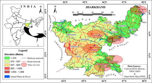
The state of Jharkhand came into existence on 15 November 2000 as the 28th state of India after being separated from the state of Bihar. The geographical area of Jharkhand is about 79,714 sq km (Bhatt 2002). Most of it lies in the periphery of the Indo-Gangetic Plain (IGP), which is considered one of the aerosol hotspots (Srivastava and Ramachandran 2013; Kumar, Tiwari, et al. 2015; Sen et al. 2017; Mhawish et al. 2017, 2018; Ramachandran et al. 2020). Jharkhand is at the centre of the Chotanagpur Plateau, about 160 km north-west of Kolkata and about 770 km south-east of Delhi. Chaibasa, Jamshedpur, Ranchi, Dhanbad, Hazaribagh, and Sahibganj are some of the major cities taken for a rigorous analysis of the variation of AOD in the context of space-time. Figure 1 covers the study area between latitudes 22° and 24.62° N and longitudes 83.26° and 87.01° E.

Figure 1. Geographical map of the study area, Jharkhand state and its major cities, India.

3. Materials and methodology

3.1. Data used

MODIS is a satellite-based global imager that can measure visible and infrared radiation in the 0.4 − 14.4 µm spectral range for land, atmosphere, and ocean applications. The data set has 36 spectral channels, and nine bands are the visible and near-infrared (NIR) spectral regions, and have wavelengths of 412 − 869 nm, and have the enhanced radiation sensibility essential for ocean colour applications (Esaias et al. 1998; Franz et al. 2007). MODIS data takes measurements at three spatial resolutions, the MODIS imagery has a spatial resolution of 250 m, 500 m, and 1 km (Kahn et al. 2009; Zhang and Reid 2009; Shi et al. 2012; Acharya and Sreekesh 2013), it takes measurements every day, and it has a wide-ranging field of view. This repetitive, widespread coverage allows MODIS data to create a widespread electromagnetic image of the world every 2 d (Miller 2003). The MODIS aerosol data products monitor the ambient aerosol stacking and some other cloud-free aerosol properties on the ocean and land surfaces. It is provided by the different types of spectral bands, and spatial observation in different algorithms have been used to retrieve the aerosol properties over the atmosphere (Kaufman et al. 1997; Levy et al. 2013; Hsu et al. 2013).

For this study, the daily transit time (∼10:30 local time, ±60 min), of average Terra-MODIS C6 AOD at 550 nm with recommended quality assurance (QA), for DT is at 10 km, DB is at 10 km, and merged DT-DB at 10 km are at the same time considered. All these products are mainly based on three algorithms: the DT algorithm over the land (Kaufman et al. 1997; Levy et al. 2013; Mhawish et al. 2017) and the DB algorithm over the ocean (Tanré et al. 1997), and the improved DB algorithm over the land (Hsu et al. 2013; Mhawish et al. 2017). Terra MODIS level 2 Dark Target aerosol data (MOD04_L2) at a spatial resolution of 3 km resolution from 2000 to 2017 were obtained from NASA’s Atmosphere Archive & Distribution System (LAADS).

The different ground-based data were used for the rigorous analysis of variation of AODs over the entire study area, such as spatial distribution of cement industries, thermal power plants (TPPs), highly polluting industries (HPIs) from Jharkhand State Pollution Control Board (Jharkhand State Pollution Control Board 2017), mines map from Indian Bureau of Mines and Google Earth Pro, forest fire from Fire Information for Resource Management System (FIRMS) (NASA 2017), road density from Open Street Map (Openstreetmap 2017), Normalized Difference Vegetation Index (NDVI) (Rouse et al. 1973; Bandyopadhyay et al. 2017; Mondal et al. 2021), and also population density from Census of India (Census of India 2011). We have considered meteorological parameters from POWER Data Access Viewer, NASA (POWER 2022), such as temperature, RH, wind speed, and wind direction, for the detailed spatial distribution and temporal trends of AOD and their correlations. Wind speed is expressed in meter per second (m/s), wind direction in degree from the north, the temperature in degree Celsius (°C), and RH in percentage (%).

3.2. Methodology

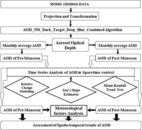
For this analysis, Terra-MODIS C6 AOD at 550 nm with recommended QA, for DT is at 10 km (corresponding to retrievals flagged QA = 3), DB is at 10 km (retrievals flagged QA ≥ 2), and merged DT-DB at 10 km are at the same time considered. AOD is derived from the MODIS Datasets (MOD04_L2) using the AOD_550_Dark_Target_Deep_Blue_Combined Algorithm. Though DT over land is not considered to retrieve AOD over bright exteriors, it is designed more accurately related to DB (in C6) over dense vegetation (Levy et al. 2013; Mhawish et al. 2017). Moreover, both DT and DB algorithms eliminate snow-covered areas but are prospective to be useful for all vegetated/transition surfaces with inconstant brightness. Therefore, a ‘best -of’ MODIS AOD products for all the transition areas was further comprised in the C6 as merged DT-DB AOD (AOD_550_Dark_Target_Deep_Blue_Combined), which is recognized considering DT over vegetated/dark-soiled land, DT over the ocean, and DB over desert/arid land (Levy et al. 2013; Mhawish et al. 2017). We have extracted a spectral signature of 550 nm from the MODIS Terra aerosol dataset (MOD04_L2), after being geo-referenced and extracted using the ENVI/IDL 5.2 software format. From these extracted AOD, we have generated an averaged AOD for pre-monsoon and post-monsoon using ERDAS IMAGINE 2014 software. Figure 2 represents the flowchart of the methodology for this study. We have extracted the level of AOD from 2000 to 2017 in pre-monsoon and post-monsoon and evaluated the space-time variation of AOD. We computed the spatial trends of AOD using the Mann − Kendall trend test (Equations (2)–(6)), Sen’s slope estimator (Equation (7)–(9)), and performed the spatial relative changes (Equation (1)(1) $$\mathrm{RPC}=\left(\frac{\mathrm{AO}{\mathrm{D}}_2-\mathrm{AO}{\mathrm{D}}_1}{\mathrm{AO}{\mathrm{D}}_1}\right)\mathrm{*}100\mathrm{ }$$(1) ), which revealed the pixel-based dynamics from a space-time perspective.

Figure 2. Flow chart of the methodology for assessing spatio-temporal trends of variation of AOD over Jharkhand state, India from 2000 to 2017.

3.2.1. Relative change analysis

To assess the variation of mean AOD in a space-time context, we have adopted the relative percentage change (RPC) statistical technique. The RPC reveals the change in AODs between the initial observations (AOD₁) and the final observations (AOD₂) in percent terms. The RPC is defined as: (1) $$\mathrm{RPC}=\left(\frac{\mathrm{AO}{\mathrm{D}}_2-\mathrm{AO}{\mathrm{D}}_1}{\mathrm{AO}{\mathrm{D}}_1}\right)\mathrm{*}100\mathrm{ }$$(1) where RPC is relative percentage changes, AOD₁ is the initial mean values of AOD, and AOD₂ is the final mean values of AOD for the conferred period.

3.2.2. Mann–Kendall (MK) trend test

Trend analysis of AOD has been investigated using the Mann-Kendall test. Mann (1945) initially used this test, and Kendall (1975) subsequently derived the test statistics distribution. Its benefit is that it is distribution-free and does not accept any unique structure for the distribution capacity of the information, including blue-pencilled and missing information and has been suggested generally by the World Meteorological Organization for public application . Subsequently, different researchers discovered the MK test to be a fantastic instrument for pattern identification in comparative applications. For the time series X₁, ., X_n, the MK Test uses the following statistic: (2) $$\mathrm{S}=\sum _{i=1}^{n-1}\sum _{j=i+1}^n\mathit{sgn}(Xj+Xi)$$(2) where n is the number of observations, x_j is the _jth observation, and sgn(^.) is the sign function which can be computed as: (3) $$\mathit{sgn}\left(x_j-x_i\right)=\{\begin{array}{c}1\mathit{\text{ if }}\left(x_j-x_i\right)>0\\ 0\mathit{\text{ if }}\left(x_j-x_i\right)=0\\ -1\mathit{\text{ if }}\left(x_j-x_i\right)<0\end{array}$$(3)

Under the assumption that the data are independent and identically distributed, the mean and variance of the S statistic in Equation (2)(2) $$\mathrm{S}=\sum _{i=1}^{n-1}\sum _{j=i+1}^n\mathit{sgn}(Xj+Xi)$$(2) are given by Kendall (1975) as: (4) $$\text{E}\left(\text{S}\right)=0$$(4) (5) $$V\left(\mathrm{S}\right)=\frac{n\left(n-1\right)\left(2n+5\right)-{\sum }_{i=1}^m{t}_i\left(t_i-1\right)\left({2t}_i+5\right)}{18}$$(5) where m is the number of groups of tied ranks, each with t_i tied observations. The original MK statistic, designated by Z, was computed as: (6) $$Z=\{\begin{array}{c}\frac{S-1}{\sqrt{Var\left(S\right)}} S>0\\ 0 S=0\\ \frac{S+1}{\sqrt{Var\left(S\right)}} S<0\end{array}$$(6)

If − Z_1−a/2 ≤ Z ≤ Z_1−a/2, then the null hypothesis of no trend was accepted at the significance level of α. Otherwise, the null hypothesis was rejected, and the alternative hypothesis was accepted at the significance level of α (Figure 2).

3.2.3. Sen’s slope estimator

Sen (1968) derived a method for estimating the Kendall Tau. This method has its application in the estimation of the slope of a linear trend, which arises from a linear equation as: (7) $$f\left(t\right)=\text{ Q}t+\text{ B}$$(7)

Here, f(t) is a function of time representing the time series, t is the time, B is constant, and Q is the slope. Q can be contracted by the equation. (8) $$Q_i=\frac{x_j-x_k}{j-k}$$(8)

Here at time j and k, j > k and i = 1, 2…, N, the values of the data pairs are represented by x_j and x_k. We can determine the median of the N values of Q_i by Rahman and Dawood (2017); (9) $$Q=\{\begin{array}{c}{Q}_{\left[\frac{N+1}{2}\right];\mathrm{ }if\mathrm{ }N\text{ is odd}}\\ \frac{1}{2}{Q}_{\left[\frac{N}{2}\right]}+Q_{\left[\frac{N+2}{2}\right]};\mathit{\text{ if N is }}\mathit{even}\end{array}$$(9)

When the value of Q_i is positive, one can discern that there is an increasing trend, and similarly, a decreasing trend shows that the value of Q_i is negative. A zero value indicates no trend (Salmi et al. 2002; Rahman and Dawood 2017).

4. Results and discussion

4.1. Evaluation of spatio-temporal trend of AOD

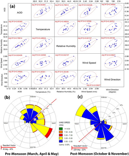
The spatio-temporal trends in AOD for the whole Jharkhand and its six major cities were assessed using the non-parametric Mann − Kendall test and Sen’s slope estimator model for the period 2000 − 2017. Here we have focused on both spatial and temporal patterns of the trend, estimated as far as changes in AOD, and further evaluated for each city area of interest. It was also assessed the correlations between aerosol emissions and meteorological factors like temperature, RH, wind speed, and wind direction. It was demonstrated a strong positive correlations were observed among these meteorological factors with aerosol emission. AOD was positively correlated with temperature (r² = 0.65), RH (r² = 0.79), wind speed (r² = 0.62), and wind direction (r² = 0.35).

4.1.1. Annual spatial trend analysis

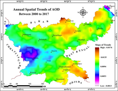
The geographical distribution of the observed trends in the AOD time series is shown in Figure 3. It is observed that each pixel exhibits an upward trend in this AOD time series analysis. The slope values of trends in AOD for the period from 2000 to 2017 are not identical over the state, it was altered between 0.0013 and 0.0176 over different places across the state. The high magnitude of the trend (Sen’s slope > 0.0135) was observed in the northern part of the state, near Satgawan, the south-western part of Sahibganj, the western part of Giridih, and the Jamshedpur region and surrounding areas. The presence of a TPP near the Satgawan region exhibits the highest AOD trend, even though the plant is located in Bihar and is closest to the Jharkhand state boundary. The south-western part of the Shibganj region demonstrates a strong positive trend of AOD for the Eastern Coal Limited (ECL) and other TPPs in relation to wind speed and wind direction which pick up the aerosol particles from the sources of aerosols and represent towards this region (Figures 10(b) and 14) (Bandyopadhyay et al. 2021). The Giridih and Jamshedpur region depicts a high level of trends due to major mining activities, TPPs, other anthropogenic activities, etc. The lower AOD trends (Sen’s slope < 0.0053) occurred over the Ganga River in the north-eastern part of the state, as the inland water body works as a sink for aerosols. The nearby Gumla, Netarhat, and Ketar regions, on the other hand, show lower AOD trends due to dense vegetation, lower population density, and very low anthropogenic activities. The remaining regions, Ranchi, Chaibasa, Balumath, Daltonganj, Hazaribagh, and Dhanbad, show moderate (Sen’s slope of 0.0053 − 0.0135) trends in AOD.

Figure 3. Annual Spatial trends of aerosol optical depth over Jharkhand state from 2000 to 2017.

However, Table 1 and Figure 4 summarize the results of the Mann − Kendall test and Sen’s slope test to determine the temporal trends and magnitude of trends of the annual AOD for six major cities in Jharkhand (Chaibasa, Jamshedpur, Ranchi, Dhanbad, Hazaribagh, and Sahibganj). It is observed that all cities have stimulated notable positive and significant trends in this period. Both Dhanbad (p value: .00190, Sen’s slope: 0.01, and Z-statistics: 3.106) and Sahibganj (p value: .00112, Sen’s slope: 0.01, and Z-statistics: 3.257) exhibit statistically significant trends at the 99% confidence level. Whereas, Chaibasa (p value: .00000, Sen’s slope: 0.011, and Z-statistics: 3.333), Jamshedpur (p value: .00000, Sen’s slope: 0.015, and Z-statistics: 3.939), Ranchi (p value: .00000, Sen’s slope: 0.009, and Z-statistics: 3.182) and Hazaribagh (p value: .00000, Sen’s slope: 0.011, and Z-statistics: 3.787) demonstrate statistically significant trends at the 99.9% confidence level. As evident from the temporal pattern of AOD in Figure 4 and Table 1, it can be representative of AOD loading, which has a statistically significant pattern with temporal variability.

Figure 4. Time series and trend lines for annual AOD over Chaibasa, Jamshedpur, Ranchi, Dhanbad, Hazaribagh, and Sahibganj of Jharkhand state from 2000 to 2017.

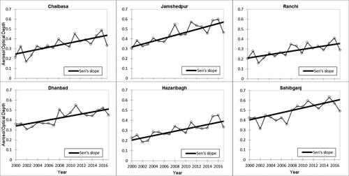
Table 1. Result of Mann–Kendal trend test and Sen’s slope estimator of annual AOD over Chaibasa, Jamshedpur, Ranchi, Dhanbad, Hazaribagh, and Sahibganj of Jharkhand state from 2000 to 2017.

City name	Kendall’s tau	p Value (two-tailed)	Sen’s slope	Std. deviation	Std. error	Z- values	Significant levels
Chaibasa	0.582	.00000	0.011	0.080	0.004437	3.3332	***
Jamshedpur	0.686	.00000	0.015	0.092	0.005103	3.9393	***
Ranchi	0.556	.00000	0.009	0.064	0.003578	3.1817	***
Dhanbad	0.542	.00190	0.010	0.072	0.004014	3.106	**
Hazaribagh	0.660	.00000	0.011	0.072	0.004004	3.7878	***
Sahibganj	0.569	.00112	0.012	0.087	0.004848	3.2575	**

Showing Kendall’s tau, p value (two-tailed), Sen’s slope, Std. deviation, Std. Error, Z-Statistics, and Significant levels

** Statistically significant trends at the 99% confidence level;

*** Statistically significant trends at the 99.9% confidence level.

4.1.2. Seasonal spatial trend analysis

The variant of AOD is very dynamic in Jharkhand, mostly associated with seasonality, which is connected with both anthropogenic and natural emissions sources. In particular, seasonal dynamics in aerosol properties are associated with local agricultural practices, livelihood, and meteorological factors like wind speed, wind direction, temperature, and precipitation. Moreover, considering such seasonal variation, aerosol loading was extracted for pre-monsoon (MAM) and post-monsoon (ON). The detailed Spatio-temporal trends of aerosol loading over Jharkhand from 2000 to 2017 by dividing them into 3-time series were analysed, which were 2000 to 2005, 2006 to 2011, and 2012 to 2017 for the pre-monsoon and post-monsoon seasons. Though it sometimes revealed increasing and decreasing trends in different short periods, over the long-term study period (2000 − 2017), the AOD loading depicted an increasing trend.

4.1.2.1. Trends of AOD in pre-monsoon

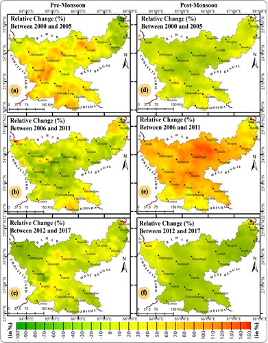
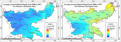
Figure 5 shows the Spatio-temporal distribution of AOD over Jharkhand state in the pre-monsoon season from 2000 to 2017. It is observed that the AOD level over the state is increasing over time due to unsustainable development in and around Jharkhand state. In 2004, the AOD level increased by 32% from the previous year in Sahibganj and it occurred again in 2008 and 2009 (Figures 5, 6(a,b), and 9(f)). Moreover, the highest AOD (0.82) was observed in the pre-monsoon over Sahibganj, and the surrounding areas in 2015, which occurred over the most densely populated area, nearest to the ECL, Rajmahal Coal Mines (RCM), nearest to the forest fire-prone area and many other local mines were validated (Figure 14(e)) (Bandyopadhyay et al. 2021) in this study. Another aspect of high AOD level over this area is there are many stone crushers, brick kilns beside the Ganga River and closest to the National Thermal Power Corporation (NTPC, Kahalgaon Power Station), which is situated near the boundary of Jharkhand (Sahibganj district) and Bihar (Figure 14(d)) (Bandyopadhyay et al. 2021). The AOD level is very high, which is thoroughly connected to the high level of coarse particles directly emitted from a series of stone crushers, besides being attributable to vast amounts of above-ground dust. It is also observed that, in case of Dhanbad and Jamshedpur regions are having much higher aerosol concentration relative to surrounding areas, due to harsh mining activity, forest fire-prone areas, highly industrialized areas, and areas close to TPPs (Figure 14(a–h)) (Bandyopadhyay et al. 2021). Figure 7 shows a thorough understanding of the AOD variants, the RPC is computed across the entire state. In conjunction with the Spatio-temporal distribution of AOD, the RPC of AOD in these regions revealed increased changes (20 − 60%). Whereas Figure 7(a–c) is represented the Sahibganj region, the RPC revealed the highest (>120%) enhancement in the AOD. The lowest AOD (0.0018) occurred in the pre-monsoon season over the middle-south-western part of the study area in 2000 between 2000 and 2017. It is covered by the eastern part of the Gumla District. In this area, vegetation cover is high (NDVI values > 0.5), less population density (< 277 per square km), low road density (< 3.5 km per square km), and there is a lack of mining activities, TPPs, and any other HPIs. These areas depicted reduced RPC (−10 to −50%) values (Figure 7(a–c)). It is also observed that the Jamshedpur region had the highest mean AOD during this period, though the Sahibganj region revealed the highest AOD in 2015. Ranchi and Hazaribagh region continuously have a low level of AOD other cities (Figures 5 and 6(a)), as these cities are far from mining activities.

Figure 5. Annual distribution of aerosol optical depth over Jharkhand state from 2000 to 2017 in pre-monsoon and post-monsoon season.

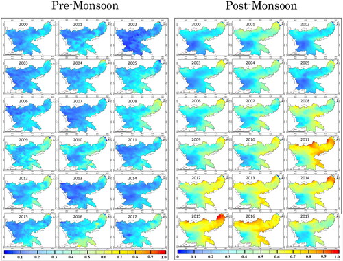
Figure 6. Box and Whisker plots showing the variation of mean AOD for pre-monsoon (a) and post-monsoon (b) seasons from 2000 to 2017 of 6 major cities of Jharkhand state; Chaibasa, Jamshedpur, Ranchi, Dhanbad, Hazaribagh, and Sahibganj represented by A–F, respectively.

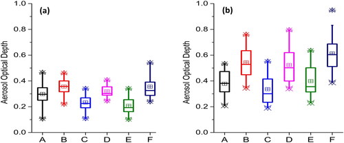
Figure 7. Pixel-based relative change of AOD for pre-monsoon (a–c) and post-monsoon (d–f) seasons over Jharkhand state for the periods between 2000 and 2017.

To reflect the detailed pattern of spatial changes in AOD and to explain the overall trend of AOD in the pre-monsoon season, we have performed the MK trend test (Equations (2)–(6)) and Sen’s slope estimator (Equations (7)–(9)) based on the mean seasonal AOD. Figure 8(a–c) indicates the calculated slopes of trends were statistically significant and provides important information relating to the long-term changes of AOD in each pixel over Jharkhand. In the case of pre-2005 (Figure 8(a)), the trends of AOD over Jharkhand in the pre-monsoon season are upward (slope > 0.025) in Jamshedpur, Dhanbad, Hazaribagh, Balumath, Giridih, and in Sahibganj the trend of AOD is maximum 0.079 (Table 2). It indicates the highly increased AOD of this area. The high upward trend illustrates that the amount of AOD is increasing with time in the Sahibganj area. As the cause of this upward trend of AOD, we can say that within this period (2000–2005), they established a lot of stone crushers coal mines (Figure 14(e)) (Bandyopadhyay et al. 2021), and brick kilns, etc. (Govt. of India, Ministry of MSME 2021). Most areas, including Daltonganj, Netarhat, Gumla, Chakradharpur, Chaibasa, Kormia, Noamundi, and others, experienced upward or positive trends during this period. Due to fewer anthropogenic activities, low population density, and dense vegetation cover, downward trends also appeared in the eastern part of the state during this period, namely Dumka, Pakur, and the eastern part of Dhanbad. In the case of the 2006–2011 time period (Figure 8(b)), the upward trends (>0.012) of AOD dominated over the North and North-West parts of Jharkhand, like Borrio, Pakur, Satgwan, Ketar, Daltonganj, and surrounding areas. Furthermore, in the Southern and slightly in the Eastern parts, like Jamshedpur, Chaibasa, Noamundi, Dhanbad, and Kormia have the positive trends of AOD. This is due to the occurrence of various anthropogenic and industrial activities in these regions. From the middle part of the state, the trends gradually increased towards the north and south of the state. Moreover, in the central part of the state, i.e. Hazaribagh, Ranchi, and surrounding areas, there are apparent negative (slope values up to −0.0705) trends in AOD. Figure 8(c) represents the periods of 2012–2017; the trends of AOD over Jharkhand are different from the previous patterns. In this period, the highest trend (0.1228) occurred in the northern part of the Sahibganj district, which is mainly covered by a lot of mining activities and stone crushers (Figure 14(e), Table 2) (Bandyopadhyay et al. 2021). These are the primary sources of aerosols. In this period, most of the area (90%) was covered by positive trends and within the very small part of the state occurred negative trends mainly covered by the North-Western part and some portions of Latehar, Lohardaga, Pakur, and Sahibganj district.

Figure 8. Seasonal Spatial trends of Aerosol Optical Depth of Pre-monsoon and Post-monsoon seasons over Jharkhand state; (a) Trends of AOD in Pre-monsoon season during 2000–2005, (b) Trends of AOD in Pre-monsoon season during 2006–2011, (c) Trends of AOD in Pre-monsoon season during 2011–2017, (d) Trends of AOD in Post-monsoon season during 2000–2005, (e) Trends of AOD in Post-monsoon season during 2006–2011, and (f) Trends of AOD in post-monsoon season during 2011–2017.

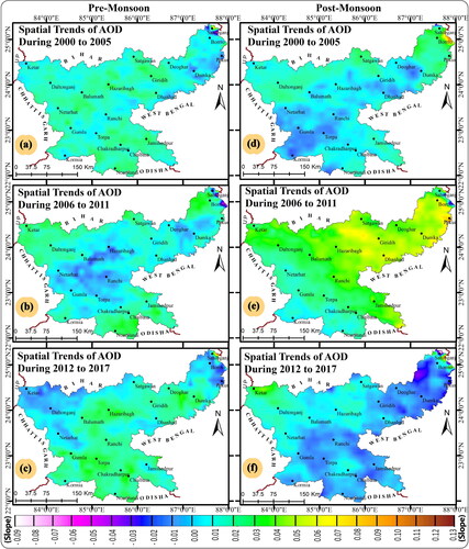
Table 2. Summary of Sen’s slope of aerosol optical depth for pre-monsoon and post-monsoon season of Jharkhand state.

Study periods	Pre-monsoon		Post-monsoon
	Highest	Lowest	Highest	Lowest
2000 to 2005	0.0794	−0.07058	0.09821	−0.05002
2006 to 2011	0.09484	−0.08291	0.10809	−0.03288
2012 to 2017	0.12288	−0.02587	0.11344	−0.09406

4.1.2.2. Trends of AOD in post-monsoon

The spatial distribution of AOD is shown in Figure 5 for the post-monsoon season from 2000 to 2017 over the Jharkhand state. Over the whole study period, the mean AOD distribution illuminated a less or more similar spatial pattern to pre-monsoon season. Although some portions have different patterns and values for AOD, A significant rise in AOD was observed over the entire state from 2008 and onwards. However, 2001, 2003, and 2006 revealed a higher level of aerosols over the Sahibganj region. It may be due to the extensive industrial activity in this region. It also observed the declining value of the AOD in 2017 (Figure 9(l)). In the post-monsoon season, the highest AOD (0.95) occurred over the western part of Godda district in 2015, which is located nearest to the ECL, RCM, and many other local mines and stone crushers (Figure 14(e)) (Bandyopadhyay et al. 2021). Another aspect of this areas high AOD is that there are a lot of brick kilns beside the Ganga River and close to the NTPC (Kahalgaon Power Station). It is situated near the boundary of Jharkhand (Sahibganj district) and Bihar, which are strongly related with high wind speed (7.52 m per second) and wind direction (towards south-south east) over this region (Figure 10(c)). The composition of all of these is responsible for the high AOD over this part of the state. The second-highest AOD level that occurred over the Dhanbad district (Figures 5 and 6(b)), which is located in the most densely populated (> 770 per square km) area and is covered by many coal mines (Figure 14(e)) (Bandyopadhyay et al. 2021). Low NDVI indicates low vegetation cover, TPPs, and high road density (> 16 km per square km). Over Dhanbad and the surrounding areas, all of these have high AODs. That’s why most of these areas have manifested increased RPC values (10 − 100%). However, between 2006 and 2011, the RPC revealed a huge rise in AOD (Figure 7(e)) in conjunction with the spatial trends within this period (Figure 8(c)). However, the lowest AOD (0.08) occurred in post-monsoon over the Western part of the Gumla district in 2006, which is mainly covered by highly dense vegetation cover (NDVI > 0.5), less population density (< 277 per square km) and there is the absence of any mines, TPPs, low road density (<3.5 km per square km) and any other HPIs. Figure 6(a,b) shows the temporal variability of AOD over six major cities. It is demonstrated that the AOD level, as well as AOD variations, are higher in the post-monsoon season than in the pre-monsoon season. When compared to Jamshedpur and Dhanbad, the Sahibganj region has the highest mean AOD. These regions have huge mining as well as industrial activities. Like in the pre-monsoon season, Ranchi and the Hazaribagh region showed a low mean AOD during the time series analysis.

Figure 9. Seasonal time series and trend lines (Mann–Kendall Trend Test) of aerosol optical depth (AOD) for six major cities of Jharkhand state from 2000 to 2017 in Pre-monsoon (a–f) and post-monsoon (g–l); (a and g) Chaibasa, (b and h) Jamshedpur, (c and i) Ranchi, (d and j) Dhanbad, (e and k) Hazaribagh, and (f and l) Sahibganj.

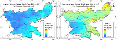
Figure 10. Scatter plot matrix and wind rose showing the correlation between AOD and meteorological parameters of Jharkhand state from 2000 to 2017; (a) correlation between AOD, temperature, relative humidity (RH), wind speed, and wind direction; (b,c) Wind rose plot of pre-monsoon and post-monsoon season, respectively, over Jharkhand state.

Figure 8(d–f) depicts the detailed spatial trends of the AOD in the post-monsoon over Jharkhand from 2000 to 2017. For rigorous analysis, we have considered three different periods, which are 2000–2005 (Figure 8(d)), 2006–2011 (Figure 8(e)) and 2012–2017 (Figure 8(f)). The period from 2000 to 2005 revealed positive trends, which occurred mainly in the northern part of the state and also in the north-east and south-east parts, which are covered by stone crushers, HPIs, etc. (Figures 8(d), 14(c,f)) (Bandyopadhyay et al. 2021). Table 2 shows the highest positive trend (0.0982) has occurred in the southeast of the Sahibganj region. Positive trends in Jharkhand covered most of the areas (75%) during this period. And the lowest trends occurred in the south-western part of the state, which is mainly covered by dense vegetation cover and rural areas of Jharkhand. Gumla, Ranchi, Torpa, and the western part of Kormia’s Noamundi block were all affected by negative trends during this period. In the period from 2006 to 2012, the spatial pattern of the trends of aerosol optical depth (AOD) was different from the previous periods. Table 2 shows the highest trends (0.108) in AOD in the Pakur region. Due to the presence of stone crushers and other HPIs (TPPs, massive mining activities, etc.), the temporal slope value of trends of AOD loading is higher than in other places. In this period, most of the areas (98%) are covered by the positive slope of trends due to anthropogenic activities. Only the areas which the Ganga River covers have a negative slope trend. As a result, we can conclude that the peak of anthropogenic activity occurred in the post-monsoon season across the entire state of Jharkhand during this period. Nevertheless, within the period from 2012 to 2017, the trends of AOD (Figure 8(f)) have revealed a contrasting picture to the previous (Figure 8(d,e)) patterns of trends. Positive trends were observed primarily in the state’s northwestern region, including the Ketar, Daltonganj, Hazaribagh, Satgwan, Balumath, and Netarhat regions. And also covered by Dhanbad, Chakradharpur, and the surrounding area. These areas exhibited a high level of mining and different industrial activities during this period. On the other hand, the decreasing trends of AOD are observed in the whole eastern part of the state, namely, Bokaro, Ramgarh, Ranchi, Jamshedpur, Dumka, Jamtara, Dewghar, Giridih, Gumla, Khunti, Topra, Chaibasa, and surrounding areas. The slope of the AOD is decreasing towards the southeast and increasing towards the northwest in the middle portion of the state.

Tables 3 and 4 show the results of the AOD trend test by the MK test and Sen’s slope test for the pre-monsoon and post-monsoon seasons, respectively, in six major cities (Chaibasa, Jamshedpur, Ranchi, Dhanbad, Hazaribagh, and Sahibganj) of Jharkhand state from 2000 to 2017. In this long-term time series analysis, it is observed that all the cities depicted positive trends in the AOD in both the seasons, pre-monsoon and post-monsoon which represented in Figure 9. Though in the pre-monsoon season (Table 3, Figure 9(a–f)) all the cities depicted upward trends, only Chaibasa and Sahibganj revealed statistically significant trends at the 95% confidence level with the slope values of 0.008, and Jamshedpur city exhibited statistically significant trends at the 99% confidence level with the slope value of 0.009. On the other hand, Ranchi, Dhanbad, and Hazaribagh showed non-significant trends, even though the trend slope of these three cities showed a positive (0.003, 0.002, and 0.004) trend in the Sen’s slope test. However, in the case of the post-monsoon season (Table 2, Figure 9(g–l)), it demonstrates a significant positive trend slope. At the 99% confidence level, Chaibasa (Sen’s slope: 0.014), and Sahibganj (Sen’s slope: 0.017) show statistically significant trends. While the MK and Sen’s slope tests revealed statistically significant trends at the 99.9% confidence level in Jamshedpur (Sen’s slope: 0.021), Ranchi (Sen’s slope: 0.017), Dhanbad (Sen’s slope: 0.021), and Hazaribagh (Sen’s slope: 0.020).

Table 3. Result of Mann–Kendal trend test and Sen’s slope estimator of AOD of pre-monsoon season over Chaibasa, Jamshedpur, Ranchi, Dhanbad, Hazaribagh, and Sahibganj of Jharkhand state from 2000 to 2017.

City name	Kendall’s tau	p Value (two-tailed)	Sen’s slope	Std. deviation	Std. error	Z- values	Significant levels
Chaibasa	0.399	.02305	0.008	0.079	0.018705	2.2727	*
Jamshedpur	0.451	.01000	0.009	0.070	0.016616	2.5757	**
Ranchi	0.137	.44872	0.003	0.058	0.013749	0.75755	H0
Dhanbad	0.111	.54449	0.002	0.054	0.012614	0.60604	H0
Hazaribagh	0.163	.36332	0.004	0.066	0.015651	0.90906	H0
Sahibganj	0.359	.04082	0.008	0.085	0.020105	2.0454	*

Showing Kendall’s tau, p value (two-tailed), Sen’s slope, Std. deviation, Std. error, Z-Statistics, and Significant levels

* statistically significant trends at the 95% confidence level;

** Statistically significant trends at the 99% confidence level;

Table 4. Result of Mann–Kendal trend test and Sen’s slope estimator of AOD of post-monsoon season over Chaibasa, Jamshedpur, Ranchi, Dhanbad, Hazaribagh, and Sahibganj of Jharkhand state from 2000 to 2017.

City name	Kendall’s tau	p Value (two-tailed)	Sen's slope	Std. deviation	Std. Error	Z- values	Significant levels
Chaibasa	0.516	.00313	0.014	0.103	0.024186	2.9545	**
Jamshedpur	0.634	.00028	0.021	0.133	0.031407	3.6363	***
Ranchi	0.595	.00065	0.017	0.112	0.026512	3.409	***
Dhanbad	0.582	.00086	0.021	0.136	0.032005	3.3332	***
Hazaribagh	0.647	.00021	0.020	0.128	0.030123	3.712	***
Sahibganj	0.477	.00639	0.017	0.145	0.034229	2.7272	**

Showing Kendall’s tau, p value (two-tailed), Sen’s slope, Std. deviation, Std. error, Z-Statistics, and Significant levels

** statistically significant trends at the 99% confidence level;

*** statistically significant trends at the 99.9% confidence level.

4.2. Seasonal characteristics of AOD

In this study, Figure 11 highlights that in assessing the seasonal characteristics and spatial distribution of AOD, we have considered only two primary seasons, pre-monsoon and post-monsoon. The multispectral MODIS time-series data over Jharkhand from 2000 to 2017 depicts the spatial distribution pattern in multi-years and is averaged with the AOD during the pre- and post-monsoons. The average spatial distribution pattern of AOD over Jharkhand is closely related to meteorological factors, such as wind direction, wind speed, temperature, and RH (Figure 10(a–c)) as well as the industrial activities, like the cement industry, mines, TPPs, forest fires, road density, brick kilns, vegetation cover (NDVI) population density, etc. (Figure 14) (Bandyopadhyay et al. 2021). The average highest AOD (0.596) is observed near the ECL, RCM in the north-eastern part of Jharkhand in pre-monsoon, whereas it has increased by 23% (AOD: 0.731) in post-monsoon. On the other hand, the lowest AOD (0.158) was observed near the Gumla in the Southwestern part of the study area in pre-monsoon, whereas in post-monsoon, it increased by 3% (AOD: 0.163).

Figure 11. Multi-year average AOD of Terra MODIS sensor for pre-monsoon and post-monsoon seasons over Jharkhand state from 2000 to 2017.

In the pre-monsoon season, the high AOD (>0.3) is observed mainly in the North-western part of the Godda and Sahibganj district, which is covered by HPIs, coal mines, brick factories, low vegetation cover, and other anthropogenic activities in this area. In addition, the depicted average wind pattern in pre-monsoon season over the state revealed a major wind direction towards north-east (resultant vector: 49 degree, 40%) (Figure 10(b)). This north-east ward wind transports the major aerosols to this region. And in the south-eastern part of the Sahibganj district, near Farakka in the Murshidabad district of West Bengal, the AOD is high, which is also nearest to the NTPC (Farraka) and the high population density (> 1334 per square km). The eastern part of Jharkhand along the state’s boundary, including most of the portions of Bokaro, Dhanbad, Jamtara, Ramgarh, Eastern Ranchi, Sarikela-Kharsawan, and Purbi-Singhbhum covered by the higher level of aerosols. The medium AOD (0.2–0.3) level is observed vertically (North to South) in the middle portion of the state, which Kodarma covers, Hazaribagh, Giridih, Ramgarh, Ranchi, Gumla, Khunti, Northern part of Chaibasa, Simdega district. The lowest AOD (0.2) was found in the Middle Western part of Jharkhand, which includes the southern parts of Daltonganj, Chatra, Garhwa, and the entire Gumla district.

In the case of post-monsoon, high AOD (>0.6) occurred along with the state of the Eastern and Northern boundaries of the state. The northern boundary is formed by the western parts of the districts of Sahibganj and Godda, as well as the northern parts of the districts of Giridih, Chatra, Kodama, and Palamu. The eastern boundary is covered by the eastern part of Sahibganj, Dhanbad, Bokaro district. Medium AOD (0.4–0.6) occurred in the maximum area of the state and covered by Ramgarh, Deoghar, Dumka, Garhwa, and Eastern part of Chaibasa, Ranchi, Hazaribagh, Giridih, Latehar districts, and Southern part of Palamu, Chatra, Kodarma and Northern part of Lohardaga and Eastern part of Khunti district. The area with the lowest AOD (<0.4) observed in the South-Western part of the state, which is covered by Gumla, Lohardaga, Simdega, Khunti and the Western part of the Chaibasa, Ranchi, Hazaribagh and Southern part of Latehar, Garhwa, and Chatra district.

Figure 12 shows the variation of AOD in two seasonal periods (pre- and post-monsoon), i.e. 2000, 2005, 2010, 2015, and 2017. In order to understand the seasonal characteristics of AOD, we performed a temporal analysis of AOD levels over Chaibasa, Jamshedpur, Ranchi, Dhanbad, Hazaribagh, and Sahibganj of Jharkhand state. Increased trends are observed throughout the year in all locations. In the case of Chaibasa, it is observed that the level of AOD is always less than 0.4 in both the seasons (i.e. in pre-and post-monsoon), except in the post-monsoon season in 2015 (AOD: 0.54). Figure 12(a) is also observed that AOD is less in post-monsoon than in the pre-monsoonal period in 2000 and 2005. The Spatio-temporal pattern recurs in the case of Ranchi and Hazaribagh. Moreover, the seasonal disparity between pre-monsoon and post-monsoon is relatively less in Chaibasa, Ranchi, and Hazaribagh region due to coequal continuous activities throughout the year (Figure 12(a,c,e), Table 5). However, in the case of Jamshedpur and the Dhanbad region, the Spatio-temporal pattern is less or more similar due to similar anthropogenic activities (mining activities) and industrially developed areas (Figure 12(b,d), Table 5). Therefore, it is observed that the level of AOD level is high in these regions of the Ranchi and the Hazaribagh region. The level of AOD is depicted in pre-monsoon and post-monsoon over the Sahibganj region in Figure 12(f). A notable temporal pattern over the Sahibganj region was observed. A positive trend from 2000 to 2015 was observed in the post-monsoon, although after 2015 it declined. But in the case of the pre-monsoon season, it continuously revealed a positive trend from 2005 to 2017. Although there is some evidence, the AOD level was highest in each location during the post-monsoon season in 2015 and lowest during the pre-monsoon season in 2000, except the Sahibganj region (AOD: 0.26 in 2005).

Figure 12. Comparative analysis of seasonal variation of AOD between pre and post-monsoonal seasons 2000, 2005, 2010, 2015, and 2017 over (a) Chaibasa, (b) Jamshedpur, (c) Ranchi, (d) Dhanbad, (e) Hazaribagh, and (f) Sahibganj of Jharkhand state.

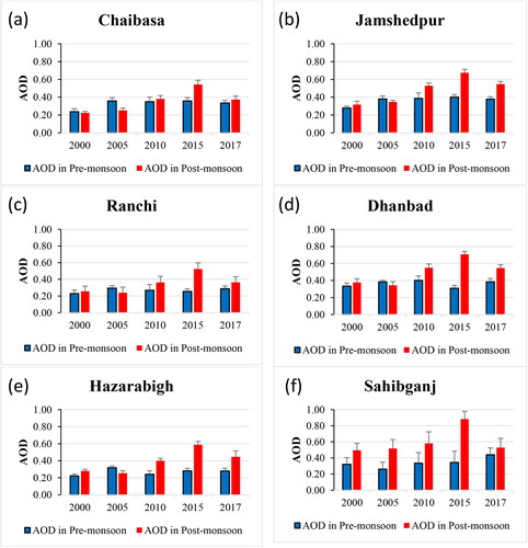
Table 5. Averaged AOD of the year 2000, 2005, 2010, 2015, and 2017 over Chaibasa, Jamshedpur, Ranchi, Dhanbad, Hazaribagh, and Sahibganj of Jharkhand state in pre- and post-monsoonal periods.

Year		AOD_2000	AOD_2005	AOD_2010	AOD_2015	AOD_2017
City name	Season	Mean ± SD	Mean ± SD	Mean ± SD	Mean ± SD	Mean ± SD
Chaibasa	Pre-monsoon	0.24 ± 0.04	0.36 ± 0.04	0.35 ± 0.05	0.36 ± 0.04	0.33 ± 0.03
	Post-monsoon	0.22 ± 0.02	0.25 ± 0.03	0.38 ± 0.04	0.54 ± 0.05	0.37 ± 0.04
Jamshedpur	Pre-monsoon	0.28 ± 0.02	0.38 ± 0.04	0.39 ± 0.06	0.40 ± 0.03	0.38 ± 0.03
	Post-monsoon	0.32 ± 0.04	0.35 ± 0.02	0.53 ± 0.03	0.67 ± 0.04	0.55 ± 0.03
Ranchi	Pre-monsoon	0.23 ± 0.04	0.29 ± 0.03	0.27 ± 0.07	0.25 ± 0.03	0.29 ± 0.03
	Post-monsoon	0.26 ± 0.06	0.24 ± 0.06	0.36 ± 0.07	0.52 ± 0.07	0.36 ± 0.07
Dhanbad	Pre-monsoon	0.33 ± 0.03	0.38 ± 0.01	0.40 ± 0.05	0.31 ± 0.03	0.38 ± 0.04
	Post-monsoon	0.38 ± 0.04	0.34 ± 0.04	0.55 ± 0.04	0.71 ± 0.03	0.55 ± 0.04
Hazaribagh	Pre-monsoon	0.22 ± 0.02	0.32 ± 0.02	0.24 ± 0.04	0.28 ± 0.03	0.28 ± 0.03
	Post-monsoon	0.28 ± 0.01	0.25 ± 0.03	0.40 ± 0.03	0.59 ± 0.04	0.45 ± 0.07
Sahibganj	Pre-monsoon	0.32 ± 0.08	0.26 ± 0.09	0.33 ± 0.13	0.34 ± 0.13	0.44 ± 0.08
	Post-monsoon	0.49 ± 0.09	0.52 ± 0.11	0.58 ± 0.14	0.88 ± 0.10	0.53 ± 0.12

4.3. Geospatial pattern of AOD over Jharkhand

The geographical distribution of the 18 years (2000–2017) of average AOD over Jharkhand is shown in Figure 13. The multi-year average spatial distribution of AOD over Jharkhand is highly correlated to this area’s physical and cultural characteristics. Such industrial zones, like the cement industry, mines, TPPs, forest fires, road density, vegetation cover (NDVI), population density, etc., are the primary regulators of the AOD (Figure 14) (Bandyopadhyay et al. 2021). Furthermore, we analysed the meteorological factors and their effects on aerosol dynamics over Jharkhand state. The high AOD loadings were found in northeast Jharkhand's industrially and economically developed areas, which are strongly correlated with the wind speed (r² = 0.62) and wind direction (r² = 0.35) (Figure 10). While the low-slung aerosol loadings were found in rural areas and a few developing areas in western and southwestern Jharkhand. The highest averaged aerosols (AOD ± SD; 0.606 ± 0.13) were found in the Northern part of Sahibganj district, which is surrounded by mining activities and HPIs (Figure 14(e)) (Bandyopadhyay et al. 2021), whereas the lowest aerosols (AOD ± SD; 0.16 ± 0.08) were found in the Western part of Gumla district, which has a lower population density (191 per square km), dense vegetation cover (>0.5), and an existing forest. The average distribution of AOD over Jharkhand is higher on the Northern and Southern boundaries of Jharkhand. And from these two different boundaries towards the South and West, the AOD is decreasing successively.

Figure 13. The geospatial pattern of average aerosol optical depth over Jharkhand state from 2000 to 2017.

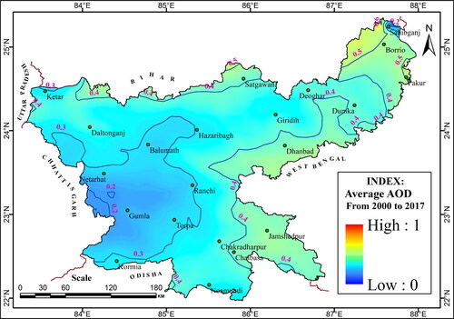
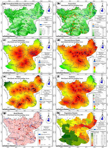
Figure 14. ‘Most important parameters for the identification of sources of aerosols: (a) spatial distribution of average NDVI; (b) forest fire (constant occurrence from 2011-2017); (c) cement industries; (d) thermal power plants; (e) mines; (f) highly polluting industries; (g) road density; and (h) population density over Jharkhand state and surrounding areas (Census of India 2011)’ (Bandyopadhyay et al. 2021).

5. Conclusions

In this study, the long-term spatio-temporal trends of MODIS AOD observed in the Indian state of Jharkhand are analysed from 2000 to 2017 using the MK trend test and Sen’s slope estimator. It was also analysed the correlations between aerosol emissions and the meteorological factors, which demonstrated strong positive correlations were observed among these meteorological factors with aerosol emission. AOD was positively correlated with temperature (r² = 0.65), RH (r² = 0.79), wind speed (r² = 0.62), and wind direction (r² = 0.35). The highest average AOD was observed in the north-eastern part of Jharkhand, which is attributed to mining activities and industrial emissions. Instead, the lowest average AOD was observed in the southwestern part of Jharkhand. A remarkable change was observed between the pre-monsoon and post-monsoon seasons.

Due to seasonal anthropogenic activities throughout the state of Jharkhand, the concentration of aerosols was higher in the post-monsoon period as compared to the pre-monsoon period. The study reported a significant change in AOD from 20 to 60%. The highest increase in AOD was recorded in Sahibganj area, where the RPC was more than 120%. All the major cities like Dhanbad, Sahibganj Chaibasa, Jamshedpur, Ranchi, and Hazaribagh exhibited a notable positive trend at ∼99% confidence level. It was observed that during the pre-monsoon season, there was an upward trend in Sahibganj and the lowest in Gumla. The temporal variation of aerosol trends was divided into three periods, namely 2000–2005, 2006–2011, and 2011–2017, revealing a remarkable transition to dominate longer-term overall trends. Interestingly, lowering of AOD on the western and southwestern borders from higher AOD on the eastern and north-eastern borders of the state was a major geospatial pattern observed in the state. Thus, this study provides an alternative approach to uncover the spatio-temporal pattern of AOD over the state of Jharkhand. In future study, it may focus on the impact of aerosol dynamics on environmental as well as human health in regional scale.

Abbreviations
AOD	=	Aerosol optical depth
DT-DB	=	Dark Target & Deep Blue
ECL	=	Eastern Coal Limited
FIRMS	=	Fire Information for Resource Management System
GDP	=	Gross Domestic Product
HPIs	=	Highly polluting industries
IGP	=	Indo-Gangetic Plain
LAADS	=	Atmosphere Archive & Distribution System
MAM	=	March, April & May
MK	=	Mann–Kendall trend test
MODIS	=	Moderate Resolution Imaging Spectroradiometer
NDVI	=	Normalized Difference Vegetation Index
NTPC	=	National Thermal Power Corporation
ON	=	October & November
RCM	=	Rajmahal Coal Mines
RH	=	Relative humidity
RPC	=	Relative Percentage Change
TPPs	=	Thermal power plants

Ethical approval

Not applicable.

Consent to participate

Not applicable.

Consent to publish

Not applicable.

Acknowledgements

The MODIS data used in this study are available at Atmosphere Archive and Distribution System (LAADS) (https://ladsweb.nascom.nasa.gov/search/), Different ground data like, Cement industries, thermal power plants (TPPs), highly polluting industries (HPIs) from Jharkhand State Pollution Control Board (Jharkhand State Pollution Control Board 2017), mines map from Indian Bureau of Mines and Google Earth Pro, forest fire from Fire Information for Resource Management System (FIRMS) (NASA 2017), road density from Open Street Map (Openstreetmap 2017) and also population density from Census of India (Census of India 2011). Meteorological parameters from POWER Data Access Viewer, NASA (POWER 2022).

Disclosure statement

This manuscript has not been published or presented elsewhere in part or in entirety and is not under consideration by another journal. There are no conflicts of interest to declare.

Lal Mohammad, Ismail Mondal: Conceptualization, Writing – original draft, Software, Formal analysis, Visualization. Jatisankar Bandyopadhyay, Quoc Bao Pham: Formal analysis; Writing – original draft, Visualization. Xuan Cuong Nguyen, Dinh Cham Dao, Ayad M. Fadhil Al-Quraishi: Supervision, Writing, Review, Editing.

Availability of data and materials

The data that support the findings of this study are available from the author, [Lal Mohammad, [email protected] and Quoc Bao Pham, [email protected]], upon reasonable request.

References

- Acharya P, Sreekesh S. 2013. Seasonal variability in aerosol optical depth over India: a spatio-temporal analysis using the MODIS aerosol product. Int J Remote Sens. 34(13):4832–4849.
- Alam K, Trautmann T, Blaschke T, Subhan F. 2014. Changes in aerosol optical properties due to dust storms in the Middle East and Southwest Asia. Remote Sens Environ. 143:216–227.
- Apte JS, Marshall JD, Cohen AJ, Brauer M. 2015. Addressing global mortality from ambient PM2.5. Environ Sci Technol. 49(13):8057–8066.
- Rahman A, Dawood M. 2017. Spatio-statistical analysis of temperature fluctuation using Mann– Kendall and Sen‟s slope approach. Clim Dyn. 48: 783–797. DOI 10.1007/s00382-016-3110-y.
- Bandyopadhyay J, Mondal I, Maiti KK, Biswas A, Acharyya A, Sarkar S, Paul A, Das P. 2017. Forest canopy density mapping for natural resource management of Jangalmahal area, India, using geospatial technology. Int J Curr Res. 9:56073–56082.
- Bandyopadhyay J, Mohammad L, Mondal I, Maiti KK, Al-Ansari N, Pham QB, Khedher KM, Anh DT. 2021. Identification and characterization the sources of aerosols over Jharkhand state and surrounding areas, India using AHP model. Geomat Nat Hazard Risk. 12(1):2194–2224.
- Banerjee T, Murari V, Kumar M, Raju MP. 2015. Source apportionment of airborne particulates through receptor modeling: Indian scenario. Atmos Res. 164:167–187.
- Banerjee T, Kumar M, Mall RK, Singh RS. 2017a. Airing ‘clean air’ in Clean India Mission. Environ Sci Pollut Res Int. 24(7):6399–6413.
- Banerjee T, Kumar M, Singh N. 2017b. Aerosol, climate and sustainability. Reference module in earth systems and environmental sciences. The encyclopaedia of anthropocene. Oxford: Elsevier.
- Biswas J, Pathak B, Patadia F, Bhuyan PK, Gogoi MM, Babu SS. 2017. Satellite-retrieved direct radiative forcing of aerosols over North-East India and adjoining areas: climatology and impact assessment. Int J Climatol. 37:298–317.
- Bhatt SC. 2002. The district Gazetteer of Jharkhand. New Delhi, India: Gyan Books.
- Boucher O, Randall D, Artaxo P, Bretherton C, Feingold G, Forster P, Kerminen VM, Kondo Y, Liao H, Lohmann U, Rasch P, Satheesh SK, Sherwood S, Stevens B, Zhang XY. 2013. Clouds and aerosols. Climate change 2013: the physical science basis. Contribution of working group I to the fifth assessment report of the intergovernmental panel on climate change. Cambridge: Cambridge University Press; p. 571–657.
- Burney J, Ramanathan V. 2014. Recent climate and air pollution impacts on Indian agriculture. Proc Natl Acad Sci USA. 111(46):16319–16324.
- Census of India. 2011. Population density, Ministry of Home Affairs. http://censusindia.gov.in.
- Charlson RJ, Langner J, Rodhe H, Leovy CB, Warren SG. 1991. Perturbation of the northern hemisphere radiative balance by backscattering from anthropogenic sulfate aerosols. Tellus A: Dyn Meteorol Oceanogr. 43(4):152–163.
- Charlson RJ, Lovelock JE, Andreae MO, Warren SGS, Schwartz JM, Hales RD, Cess JA, Coakley Jr., JE, Hansen, DJ, Hofmann. 1992. Climate forcing by anthropogenic aerosols. Science. 255(5043):423–430.
- Creamean JM, Suski KJ, Rosenfeld D, Cazorla A, DeMott PJ, Sullivan RC, White AB, Ralph FM, Minnis P, Comstock JM, et al. 2013. Dust and biological aerosols from the Sahara and Asia influence precipitation in the western US. Science. 339(6127):1572–1578.
- Dubovik O, Holben B, Eck TF, Smirnov A, Kaufman YJ, King MD, Tanré D, Slutsker I. 2002. Variability of absorption and optical properties of key aerosol types observed in worldwide locations. J Atmos Sci. 59(3):590–608.
- Englert N. 2004. Fine particles and human health-a review of epidemiological studies. Toxicol Lett. 149(1-3):235–242.
- Esaias WE, Abbott MR, Barton I, Brown OB, Campbell JW, Carder KL, Clark DK, Evans RH, Hoge FE, Gordon HR, et al. 1998. An overview of MODIS capabilities for ocean science observations. IEEE Trans Geosci Remote Sens. 36(4):1250–1265.
- Evgenieva T, Wiman BLB, Kolev NI, Savov PB, Donev EH, Ivanov DI, Danchovski V, Kaprielov BK, Grigorieva VN, Iliev I, et al. 2011. Three-point observation in the troposphere over Sofia-Plana Mountain, Bulgaria. Int J Remote Sens. 32(24):9343–9363.
- Franz BA, Kwiatkowska EJ, Meister G, McClain CR, James J, Butler, Jack X. 2007. Utility of MODIS–Terra for ocean color applications, earth observing systems XII. SPIE Vol. 6677, 66700Q, SPIE Proceedings [SPIE Optical Engineering, Applications - San Diego, CA (Sunday 26 August 2007)]. DOI: 10.1117/12.732082
- Fraser MP, Yue ZW, Buzcu B. 2003. Source apportionment of fine particulate matter in Houston, TX, using organic molecular markers. Atmos Environ. 37(15):2117–2123.
- Götschi T, Heinrich J, Sunyer J, Künzli N. 2008. Long-term effects of ambient air pollution on lung function: a review. Epidemiology. 19(5):690–701.
- Govt. of India, Ministry of MSME. 2021. Br. MSME-Development Institute (Ministry of MSME, Govt. of India), 1-18. http://dcmsme.gov.in/old/dips/Sahibganj.pdf.
- Guleria RP, Kuniyal JC, Rawat PS, Thakur HK, Sharma M, Sharma NL, Singh M, Chand K, Sharma P, Thakur AK, et al. 2011. Aerosols optical properties in dynamic atmosphere in the northwestern part of the Indian Himalaya: a comparative study from ground and satellite based observations. Atmos Res. 101(3):726–738.
- Guleria RP, Kuniyal JC, Rawat PS, Thakur HK, Sharma M, Sharma NL, Dhyani PP, Singh M. 2012. Validation of MODIS retrieval aerosol optical depth and an investigation of aerosol transport over Mohal in north western Indian Himalaya. Int J Remote Sens. 33(17):5379–5401.
- Guleria RP, Kuniyal JC, Dhyani PP. 2012. Validation of space-born Moderate Resolution Imaging Spectroradiometer remote sensors aerosol products using application of ground-based Multi-wavelength Radiometer. Adv Space Res. 50(10):1391–1404.
- Guleria RP, Chand K. 2020. Emerging patterns in global and regional aerosol characteristics: a study based on satellite remote sensors. J Atmos Sol Terr Phys. 197:105177.
- Gupta R, Somanathan E, Dey S. 2017. Global warming and local air pollution have reduced wheat yields in India. Clim Change. 140(3–4):593–604.
- Ho KF, Cao JJ, Lee SC, Chan CK. 2006. Source apportionment of PM2. 5 in urban area of Hong Kong. J Hazard Mater. 138(1):73–85.
- Hsu NC, Jeong M-J, Bettenhausen C, Sayer AM, Hansell R, Seftor CS, Huang J, Tsay S-C. 2013. Enhanced Deep Blue aerosol retrieval algorithm: the second generation. J Geophys Res Atmos. 118(16):9296–9315.
- IPCC. 2013. Climate change 2013: the physical science basis. Cambridge: Cambridge University Press.
- Jharkhand State Pollution Control Board. 2017. Polluted industry. https://www.jspcb.nic.in/upload/5d6cabafc0dec5bd05a060aaefUpdated_list_of_17_Cat._of_highly_polluting_Ind._and_calibration.pdf.
- Kahn RA, Nelson DL, Garay MJ, Levy RC, Bull MA, Diner DJ, Martonchik JV, Paradise SR, Hansen EG, Remer LA. 2009. MISR aerosol product attributes and statistical comparisons with MODIS. IEEE Trans Geosci Remote Sens. 47(12):4095–4114.
- Kahn RA, Gaitley BJ, Garay MJ, Diner DJ, Eck TF, Smirnov A, Holben BN. 2010. Multiangle imaging spectro radiometer global aerosol product assessment by comparison with the aerosol robotic network. J Geophys Res. 115(D23):23209.
- Kappos AD, Bruckmann P, Eikmann T, Englert N, Heinrich U, Höppe P, Koch E, Krause GHM, Kreyling WG, Rauchfuss K, et al. 2004. Health effects of particles in ambient air. Int J Hyg Environ Health. 207(4):399–407.
- Kaufman YJ, Wald AE, Remer LA, Gao BC, Li RR, Flynn L. 1997. The MODIS 2.1-/spl mu/m channel-correlation with visible reflectance for use in remote sensing of aerosol. IEEE Trans Geosci Remote Sens. 35(5):1286–1298.
- Kaufman YJ, Tanré D, Boucher O. 2002. A satellite view of aerosols in the climate system. Nature. 419(6903):215–223.
- Kaufman YJ, Koren I, Remer LA, Rosenfeld D, Rudich Y. 2005. The effect of smoke, dust, and pollution aerosol on shallow cloud development over the Atlantic Ocean. Proc Natl Acad Sci USA. 102(32):11207–11212.
- Kaufman YJ, Boucher O, Tanré D, Chin M, Remer LA, Takemura T. 2005. Aerosol anthropogenic component estimated from satellite data. Geophys Res Lett. 32(17):L17804.
- Kaur P, Dhar P, De BK, Guha A. 2020. Inter-comparison of satellite retrieved Aerosol Optical Depth (AOD) from geostationary and polar-orbiting platforms with ground-based measurements over a Semi-continental site of north-eastern India. 2020 URSI regional conference on radio science (URSI-RCRS). Piscataway (NJ): IEEE;. p 1–4.
- Kendall MG. 1975. Rank correlation methods. London: Charles Griffin; p. 202.
- Kulmala M, Kontkanen J, Junninen H, Lehtipalo K, Manninen HE, Nieminen T, Petäjä T, Sipilä M, Schobesberger S, Rantala P, et al. 2013. Direct observations of atmospheric aerosol nucleation. Science. 339(6122):943–946.
- Kumar M, Singh RS, Banerjee T. 2015. A review on the human health impact of airborne particulate matter. Environ Int. 74(2015):136–143.
- Kumar M, Tiwari S, Murari V, Singh AK, Banerjee T. 2015. Wintertime characteristics of aerosols at middle Indo-Gangetic Plain: Impacts of regional meteorology and long range transport. Atmos Environ. 104:162–175.
- Kumar R, Guleria RP. 2017. A review of potential radiative effect of aerosol on climate. Indian J.Radio Space Phys. 46(1):5–14.
- Kumar M, Raju MP, Singh RS, Banerjee T. 2017. Impact of drought and normal monsoon scenarios on aerosol induced radiative forcing and atmospheric heating in Varanasi over middle Indo-Gangetic Plain. J Aerosol Sci. 113:95–107.
- Kumar M, Raju MP, Singh RK, Singh AK, Singh RS, Banerjee T. 2017. Wintertime characteristics of aerosols over middle indo-gangetic plain: vertical profile, transport and radiative forcing. Atmos Res. 183:268–282.
- Kuniyal JC, Guleria RP. 2019. The current state of aerosol-radiation interactions: a mini review. J Aerosol Sci. 130:45–54.
- Lelieveld J, Evans JS, Fnais M, Giannadaki D, Pozzer A. 2015. The contribution of outdoor air pollution sources to premature mortality on a global scale. Nature. 525(7569):367–371.
- Levy RC, Mattoo S, Munchak LA, Remer LA, Sayer AM, Patadia F, Hsu NC. 2013. The Collection 6 MODIS aerosol products over land and ocean. Atmos Meas Tech. 6(11):2989–3034.
- Lu Z, Zhang Q, Streets DG. 2011. Sulfur dioxide and primary carbonaceous aerosol emissions in China and India, 1996–2010. Atmos Chem Phys. 11(18):9839–9864.
- Mann HB. 1945. Nonparametric tests against trend. Econometrica. 13(3):245–259.
- Mehta M. 2015. A study of aerosol optical depth variations over the Indian region using thirteen years (2001–2013) of MODIS and MISR Level 3 data. Atmos Environ. 109:161–170.
- Mehta M, Khushboo R, Raj R, Singh N. 2021. Spaceborne observations of aerosol vertical distribution over Indian mainland (2009–2018). Atmos Environ. 244:117902.
- Menon S, Hansen J, Nazarenko L, Luo Y. 2002. Climate effects of black carbon aerosols in China and India. Science. 297(5590):2250–2253.
- Mhawish A, Banerjee T, Broday DM, Misra A, Tripathi SN. 2017. Evaluation of MODIS Collection 6 aerosol retrieval algorithms over indo-gangetic plain: implications of aerosols types and mass loading. Remote Sens Environ. 201:297–313.
- Mhawish A, Kumar M, Mishra A. K, Srivastava PK, Banerjee T. 2018. Remote sensing of aerosols from space: retrieval of properties and applications. Remote sensing of aerosols, clouds, and precipitation. Amsterdam, Netherlands: Elsevier. p. 45–83.
- Miller SD. 2003. A consolidated technique for enhancing desert dust storms with MODIS. Geophys Res Lett. 30(20):2071.
- Ministry of Statistics and Program Implementation | Government of India. 2017. mospi.nic.in. on 4 March 2016. Retrieved 28 September, 1-54. http://mospi.nic.in
- Mondal I, Thakur S, Juliev M, De TK. 2021. Comparative analysis of forest canopy mapping methods for the Sundarban biosphere reserve, West Bengal, India. Environ Dev Sustain. 23(10):15157–15182..
- Mondal I, Thakur S, De A, De TK. 2022. Application of the METRIC model for mapping evapotranspiration over the Sundarban Biosphere Reserve, India, Ecological Indicators. Amsterdam, Netherlands: Elsevier; p. 108553..
- More S, Kumar PP, Gupta P, Devara PCS, Aher GR. 2013. Comparison of aerosol products retrieved from AERONET, MICROTOPS and MODIS over a tropical urban city, Pune, India. Aerosol Air Qual Res. 13(1):107–121.
- NASA Earth Observation. 2021. Aerosol Optical Depth. . https://neo.sci.gsfc.nasa.gov/view.php?datasetId=MODAL2_M_AER_OD.
- NASA. 2017. Fire Information for Resource Management System LANCE, University of Maryland. https://firms.modaps.eosdis.nasa.gov/
- Obregón MA, Costa MJ, Silva AM, Serrano A. 2020. Spatial and temporal variation of aerosol and water vapour effects on solar radiation in the Mediterranean basin during the last two decades. Remote Sens. 12(8):1316.
- Openstreetmap. 2017. Road Density. https://wiki.openstreetmap.org/wiki/Main_Page.
- Pandolfi M, Cusack M, Alastuey A, Querol X. 2011. Variability of aerosol optical properties in the Western Mediterranean Basin. Atmos Chem Phys. 11(15):8189–8203.
- POWER. 2022. Data access viewer, NASA. https://power.larc.nasa.gov/data-access-viewer/.
- Provençal S, Kishcha P, da Silva AM, Elhacham E, Alpert P. 2017. AOD distributions and trends of major aerosol species over a selection of the world’s most populated cities based on the 1st version of NASA's MERRA Aerosol Reanalysis. Urban Clim. 20:168–191.
- Ramanathan VCPJ, Crutzen PJ, Kiehl JT, Rosenfeld D. 2001. Aerosols, climate, and the hydrological cycle. Science. 294(5549):2119–2124.
- Ramachandran S, Kedia S, Srivastava R. 2012. Aerosol optical depth trends over different regions of India. Atmos Environ. 49:338–347.
- Ramachandran S, Rupakheti M, Lawrence MG. 2020. Black carbon dominates the aerosol absorption over the Indo-Gangetic Plain and the Himalayan foothills. Environ Int. 142:105814.
- Ramanathan V, Crutzen PJ, Lelieveld J, Mitra AP, Althausen D, Anderson J, Andreae MO, Cantrell W, Cass GR, Chung CE, et al. 2001. Indian ocean experiment: an integrated analysis of the climate forcing and effects of the great Indo-Asian haze. J Geophys Res. 106(D22):28371–28398.
- Ramanathan V, Chung C, Kim D, Bettge T, Buja L, Kiehl JT, Washington WM, Fu Q, Sikka DR, Wild M. 2005. Atmospheric brown clouds: impacts on South Asian climate and hydrological cycle. Proc Natl Acad Sci USA. 102(15):5326–5333.
- Remer LA, Kaufman YJ, Tanré D, Mattoo S, Chu DA, Martins JV, Li R-R, Ichoku C, Levy RC, Kleidman RG, et al. 2005. The MODIS aerosol algorithm, products, and validation. J Atmospher Sci. 62(4):947–973.
- Rouse JW, Haas RH, Schell JA, Deering DW. 1973. Monitoring vegetation systems in the Great Plains with ERTS. 3rd ERTS Symposium, NASA SP-351, Washington DC, 10-14 December 1973, I. p. 309–317.
- Salmi T, Määttä A, Anttila P, Ruoho-Airola T, Amnell T. 2002. Detecting trends of annual values of atmospheric pollutants by the Mann-Kendall test and Sen’s slope estimates MAKESENS–The excel template application. Helsinki, Finland: Finish Meteorological Institute.
- Seinfeld JH, Bretherton C, Carslaw KS, Coe H, DeMott PJ, Dunlea EJ, Feingold G, Ghan S, Guenther AB, Kahn R, et al. 2016. Improving our fundamental understanding of the role of aerosol − cloud interactions in the climate system. Proceedings of the National Academy of Sciences of the United States of America, 113 (21): 5781–5790. doi:10.1073/pnas.1514043113
- Sen A, Abdelmaksoud AS, Nazeer Ahammed Y, Alghamdi M ِ, Banerjee T, Bhat MA, Chatterjee A, Choudhuri AK, Das T, Dhir A, et al. 2017. Variations in particulate matter over Indo-Gangetic Plains and Indo-Himalayan Range during four field campaigns in winter monsoon and summer monsoon: role of pollution pathways. Atmos Environ. 154:200–224.
- Sen PK. 1968. Estimates of the regression coefficient based on Kendall’s tau. J Am Stat Assoc. 63(324):1379–1389.
- Sheel V, Guleria RP, Ramachandran S. 2018. Global and regional evaluation of a global model simulated AODs with AERONET and MODIS observations. Int J Climatol. 38:e269–e289.
- Shi Y, Zhang J, Reid JS, Liu B, Deshmukh R. 2012. Critical evaluation of cloud contamination in MISR aerosol product using collocated MODIS aerosol and cloud products. Atmos Meas Tech. 7:A13J–0310.
- Srivastava R, Ramachandran S. 2013. The mixing state of aerosols over the Indo‐Gangetic Plain and its impact on radiative forcing. QJR Meteorol Soc. 139(670):137–151.
- Srivastava R, Bran SH. 2017. Spatio‐temporal variations of black carbon and optical properties in a regional climate model. Int J Climatol. 37(3):1432–1443.
- Stachlewska IS, Zawadzka O, Engelmann R. 2017. Effect of heat wave conditions on aerosol optical properties derived from satellite and ground-based remote sensing over Poland. Remote Sens. 9(11):1199.
- Su J, Huang J, Fu Q, Minnis P, Ge J, Bi J. 2008. Estimation of Asian dust aerosol effect on cloud radiation forcing using Fu-Liou radiative model and CERES measurements. Atmos Chem Phys. 8(10):2763–2771.
- Tanré D, Kaufman YJ, Herman M, Mattoo S. 1997. Remote sensing of aerosol properties over oceans using the MODIS/EOS spectral radiances. J Geophys Res. 102(D14):16971–16988.
- Tripathi SN, Pattnaik A, Dey S. 2007. Aerosol indirect effect over Indo-Gangetic plain. Atmos Environ. 41(33):7037–7047.
- WHO. 2014. Burden of disease. Geneva, Switzerland: World Health Organization. [accessed on 10 February 2017]. http://www.who.int/gho/phe/outdoor_air_pollution/urden_text/en/.
- Zhang J, Reid JS. 2009. An analysis of clear sky and contextual biases using an operational over ocean MODIS aerosol product. Geophys Res Lett. 36(15):n/a–n/a.
- Zhang YL, Cao F. 2015. Fine particulate matter (PM 2.5) in China at a city level. Sci Rep. 5(1):1–12.