Land use/cover spatiotemporal dynamics, and implications on environmental and bioclimatic factors in Chingola district, Zambia

Abstract

This study uses remote sensing and GIS techniques to examine the intensity and dynamics of land use/cover change and environmental indices across a four-decade period in the Chingola district of Zambia, from 1972 to 2020 using five classification stages (1972, 1992, 2001, 2013, and 2020). A total of 10 key climate change detection monitoring indices were generated using RClimDex to examine the implications of land degradation on the bioclimatic factors from 1983 to 2020. The findings revealed a significant expansion in Built-ups (7.3%/year), farmlands (3.18%/year), and mining areas (0.82%/year) at the expense of natural resources. The highest human pressure was exerted on Savannah woodlands (−0.78), through agriculture (0.76) and infrastructure development (0.44) between 1992 and 2001.The analysis of the bioclimatic indices revealed a significant decline in rainfall quantity and intensity, and a rising in temperature (warmer days and nights). The Annual rainfall has decreased by −3.25%, while the potential evapotranspiration has increased by 0.04% from 1983 to 2020, resulting in an Aridity Index of 0.60 and a moisture deficit index of −0.42. To offset agriculture’s propensity to spatially expand and further encroach into savannah woodlands and forests, urban containment policies and programs that stimulate agricultural intensification are needed to reduce urban sprawl and protect the city’s remaining forestlands.

Highlights

• The most significant changes in LULC in Chingola occurred between 2001 and 2013 with a CLUDI of (623).

• It was observed that the days and nights are becoming warmer given the trend TX90p and TN90p.

• The PET analysis showed the years 1999, 2000, 2005, and 2017 with the greatest rainfall deficits.

• A declining trend was observed in NDVI, NDWI, NDMI, and NDSI over the study period (1972–2020).

• The highest human pressure was exerted on Savannah woodlands with an urban sprawl index of (−0.78).

• The year 1998 was identified as the hottest and driest of 1983–2020 timeseries.

Keywords:

• Chingola
• Urban sprawl
• climate change
• land use/land cover
• environmental factors

1. Introduction

In regions with extensive mining activities, several anthropogenic disturbances alter directly and indirectly the landscape (Leal et al. 2012; Liu and Wang 2014; Li et al. 2015), destroying the natural forest and habitats of many species and modifying the ecosystem functions (Lambin et al. 2003; Meyfroidt et al. 2013), polluting the air, soil, and water (Skalos and Kasparova 2012; DeWitt et al. 2017; Kourouma et al. 2019). Biomes such as forests, savannah woodlands, and wetlands are mainly subject to fragmentation (Batar et al. 2017), exacerbated by population growth, increased demands for biofuels and food crops.

Zambia in general and Chingola district have had their landscape dominated by mining activities since 1928 (Nakayama et al. 2011; Ncube et al. 2012; Kribek et al. 2014; Lindahl 2014) characterized by large open pits, deep shafts, large volume waste disposal, tailing dams, and pyrometallurgical processing facilities, posing significant impacts on the environment in terms of air pollution, siltation of rivers, land contamination with heavy metals and habitat destruction (Limptlaw 2003). The spatial extent, temporal dynamics and cumulative effects of land use and land cover change on the climate and environment are not well understood in Africa in general and Zambia in particular.

Land use and land cover change are one of the main contributors to global warming (Linda and Oluwatola 2015), through deforestation that contribute to greenhouse gases. The rise in temperature in Africa is projected to range between 4 and 6 °C in the subtropics and between 3 to 5 °C in the tropics by the end of the century (Engelbrecht et al. 2015; Nangombe et al. 2018). This is expected to exacerbate the number of extreme weather events, such as drought, floods and heatwaves (Polioptro and Bandala 2018), which are already occurring more frequently, intensely, and are lasting longer than before (Perkins et al. 2012).

Moreover a city hosting a mining industry such as Chingola, is subject to a consistent rise in air and land surface temperature and Urban Heat Islands (UHI) phenomena that trap the local air pollution and humidity, decreasing labor productivity and making it difficult for those with respiratory illness to breathe properly and possibly die of heat stroke (Filleul et al. 2006; Kjellstrom et al. 2009, 2014, Kjellstrom 2016; Hollowell 2010; Tomlinson et al. 2011; Lucas et al. 2014; Gun 2019; Vaidyanathan et al. 2020). However, very few research has been done on industrial air pollution and its impact on the environment and human health in Zambia. Ncube et al. (2012) on the Copperbelt province, reported that copper smelting activities result in atmospheric emissions between 300,000 and 700,000 tons/year, far above the WHO limit of 125,000 tons/year. Having a clear grasp of how the local environment and microclimate are changing and the linkages between the changing environmental and bioclimatic factors in the context of global warming is very important to adopt adequate and efficient sectoral adaptation strategies. To fully grasp the effects of urbanization on local environment, human comfort and health which are linked to the magnitude of urban heat and cold islands, as well as changes in the bioclimatic and environmental factors, fine-scale data is required, which is typically not available in most developing countries, including Zambia (WHO 2017; Wichmann 2017; Nana et al. 2019; WMO 2021).

Moreover, the lack of reliable data has coincided with a period of rapid urbanization around the world, and policymakers and urban planners have been advocating for solutions to bridge this information gap. Monitoring LULC changes in the mining areas are crucial to providing valuable information for the management of the landscape and how to prioritize the interventions (Weiers et al. 2004; Curatola et al. 2015; Jorgenson and Fraumeni 2020). The use of remotely sensed satellite imagery has been found helpful in resolving limitations associated with traditional surveying methods for tracking long-term changes in LULC. They have the advantage of being cost-effective, freely available, and provide the possibility to track change in land use and land cover over a long temporal scale (Lambin 2003; Patel et al. 2017; Phiri and Morgenroth 2017; Huang et al. 2019; Hoque et al. 2020), with special attention to mining areas (Schmidt 2010; Phiri 2020). In the Chingola district, land use planning processes are greatly inhibited by insufficient data availability, which is a common issue in developing countries (Potts 2012; Schug et al. 2018). Therefore, studies of land use and land cover change and related changes of environmental and bioclimatic factors such as temperature, rainfall and evapotranspiration, are relevant in countries such as Zambia where there are inadequate preventive and control measures. This study aims specifically, to (1) Analyze the magnitude, intensity, and dynamics of change among land cover categories (2) Analyze how population growth affects each land use category (3) Analyze how LULC and subsequent changes in the local climate has affected the environmental and bioclimatics factors; (4) to propose preventive and mitigation measures to avoid future undesirable impacts of land use and land cover change and Climate change.

This study used both spatial and non-spatial methods to provide insight on the current trend of environmental and bioclimatic factors in the mining district of Chingola in the context of climate change, and population growth. It has, therefore, the potential to have an important scientific contribution through the exposition of patterns, characteristics of change in land use and land cover, and the implications of the changes in bioclimatic and environmental factors in mining areas which have never been addressed by previous studies. One of the practical contributions is to alert and inform government and local community abreast with current trends and status on the climate and environmental indicators and advise on the future direction to be taken by policymakers and decision-makers toward achieving the United Nation’s Sustainable Development Goals 3, 11, and 13 for improved health and wellbeing, sustainable cities, and climate actions respectively.

2. Materials and methods

2.1. Description of the study area

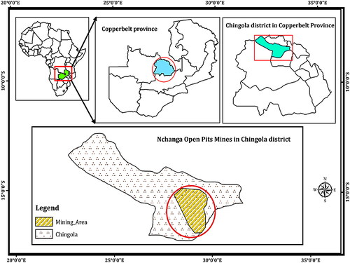
Chingola district is in the Copperbelt Province of Zambia (Figure 1) and lies between 12°20′ South and 27°50′ East and has an elevation of 1300 m above sea level. The Copperbelt mining area is about 120 km long and 50 km wide, stretching from Konkola in the Northwest to Luanshya in the southeast (Limpitlaw 2001). Since 1928, Copper mining in Zambia has contributed to the economic transformation and has been a major component of the Gross Domestic Product (GDP), with more than 80% of the country's foreign exchange earnings, over 50% of government revenue, and at least 20% of total employment (Simutanyi 2008; Kabemba 2014). Chingola landscape has been significantly impaired by mining activities, with large areas occupied by overburdened materials, large volumes of waste rocks, and huge open pits, one of the deepest in the world. The climatic condition in Copperbelt Province is characterized by three distinct seasons namely (i) warm a dry season (August to November), (ii) Warm wet season (November to April), and (iii) cold dry season (May to August). The district lies in Region III of the agro-ecological zone, and the average rainfall ranges from 1000 mm to 1200 mm, while the mean temperatures range from 10 °C to 37 °C (DPU 2019). The prevailing winds are mostly south-easterly in the dry season and north-westerly during the rainy season. Soils of Copperbelt province, according to the FAO classification belong to the group of ferrasols (acric, orthic or rhodic ferrasols) (FAO-UNESCO 1997). The principal soil-forming process in the area is rock weathering; hence, climatic factors influence the rate and depth of weathering and soil formation. Chingola mineral ores are hosted by arenites and argillites of the Lower Roan Subgroup with a geological formation belonging to the Phanerozoic Lufilian Fold Belt (LFB). The LFB forms part of a series of linked Pan-African orogenic belts fringing the Congo and Kaapvaal-Zimbabwe craton of Southern Africa (Selley 2005; McGowan 2006). The major vegetation type is miombo woodlands. The dominant species include Brachystegia spp., Isoberlinia angolensis, and Julbernardia paniculata.

Figure 1. Location map of Chingola district in the Copperbelt province of Zambia.

The total population of Chingola is estimated at 182,231 inhabitants, with females accounting for 49.9% and males 50.01% (Central Statistics Office [CSO] 2020). The average annual population growth rate stands at 2.3% (DPU 2019). The peri-urban areas of the district are sparsely populated, with mining and agriculture as the main economic activities (DPU 2019).

2.2. Remotely sensed data

Data collection involved image acquisition, image pre/processing, classification, accuracy assessment, and change detection. Figure 2 presents the summary of the steps followed in data collection.

Figure 2. Flowchart of the methodology used in the study.

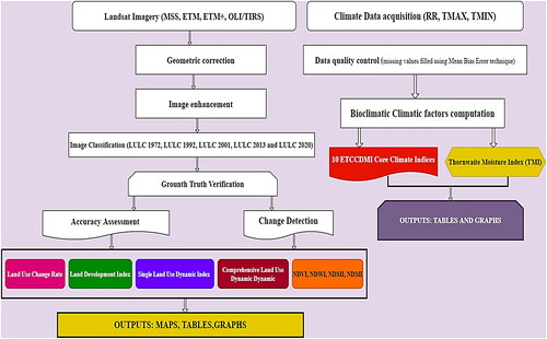
Landsat 1 Multispectral Scanner (MSS) of 1972, Landsat 5 Thematic Mapper (TM) of 1992, Landsat 7 Enhanced Thematic Mapper Plus (ETM+) of 2001, and Landsat 8 Operational Land Imager (OLI) and the Thermal Infrared Sensor (TIRS) (OLI/TRIS) datasets of 2013 and 2020 with their respective paths and rows [(185, 069); (172, 068); (172, 069)] (Table 1) were used in the study. This dataset was acquired from the United States Geological Survey (USGS) website (https://earthexplorer.usgs.gov) and used to evaluate LULC changes in Chingola. Images from August and September, during the dry season when clouds are minimal, were selected for this study (Table 1).

Table 1. List of Landsat images used in the study.

Sensor	Date of acquisition	Spatial resolution (m)	Path/Row	Producer
Landsat MSS	1972/09/13	60	185/069	USGS
Landsat 5 ETM	1992/08/29	30	172/068, 172/069	USGS
Landsat 7 ETM+	2001/08/14	30	172/068, 172/069	USGS
Landsat 8 OLI/TIRS	2013/09/08	30	172/068, 172/069	USGS
Landsat 8 OLI/TIRS	2018/09/12	30	172/068, 172/069	USGS

OLI: Operation Land Imager; USGS: United States Geological Survey; MSS: Multispectral Scanner System; TM: Thematic Mapper.

2.2.1. Data processing and analysis

Image pre-processing and post-classification

The satellite images were imported and pre-processed using ENVI 5.3 software. The images were first converted to radiance values, all stacked except for the thermal infrared band (i.e. Band 6), and then, atmospheric image calibration was applied for the USGS guide. The Landsat image of 1992 was used as a base for empirical line normalization (ENVI User's Guide 2008). Geometric rectification, image co-registration in the common spatial frame reference (in this case to WGS ellipsoid projection) as suggested by (Schmidt and Glaesser 1998), thereafter radiometric calibration, and topographic correction were applied to all images to minimize the errors. These techniques have been widely applied and are considered the most suitable algorithms for minimizing errors when pre-processing satellite images (USGS 2016; Ranagalage et al. 2017; Singh et al. 2017; Chaudhuri et al. 2018). Landsat images were projected to a common coordinated system, World Geodetic System (WGS) 84, Zone 35 North. Before classification, we used spectral signatures to ascertain the separability of digital numbers (DN) of different LULC categories. The DN conversion using the Gain and Bias method to convert the DN value to radiance using the formula below: $$L_{\lambda }=\mathit{gain}\mathrm{\hspace{0.17em}*\hspace{0.17em}}DN+\mathit{bias}$$ where $L_{\lambda }$ is the cell value as radiance; DN is the cell value digital number; gain is the gain value for a specific band; bias is the bias value for a specific band.

Thereafter the radiance values obtained were converted to a ToA reflectance value using the formula below: $${\rho }_{\lambda }=\mathit{\pi }\mathrm{\hspace{0.17em}*\hspace{0.17em}}{L}_{\lambda }\mathrm{\hspace{0.17em}*\hspace{0.17em}}\frac{d^2}{{\mathit{ESUN}}_{\lambda }}\mathrm{\hspace{0.17em}*\hspace{0.17em}}\hspace{0.17em}\mathit{\text{cos}}\hspace{0.17em}{\mathit{\theta }}_{\mathit{s}}$$ ${\rho }_{\lambda }=\mathit{Unitless}\mathrm{ }\mathit{planetary}\mathrm{ }\mathit{reflectance};\mathrm{ }{L}_{\lambda }=\mathit{spectral}\mathrm{ }\mathit{radiance}\mathrm{ }\left(\mathit{from}\mathrm{ }\mathit{earliest}\mathrm{ }\mathit{step}\right);d=\mathit{Earth}-\mathit{Sun}\mathrm{ }\mathit{distance}\mathrm{ }in\mathrm{ }\mathit{astronmoical}\mathrm{ }\mathit{units};$ ${\mathit{ESUN}}_{\lambda }=\mathit{mean}\mathrm{ }\mathit{solar}\mathrm{ }\mathit{exoatmospheric}\mathrm{ }\mathit{irradiances};\mathrm{ }{\theta }_s=\mathit{solar}\mathrm{ }\mathit{zenith}\mathrm{ }\mathit{angle}.$

Eighty training sites, ranging from 350 to 900 pixels, were used to train the images. Training samples included 20–40 subclasses for each class. After image pre-processing (normalization, histogram equalization, noise filtering, and image segmentation) in ENVI v.5.3, a supervised classification using class hierarchy and accuracy assessment was done in eCognition. All maps of land use and land cover change and environmental indices were done in ArcGIS v.10.8. These methods and techniques have used and recommended by many scholars (Yang et al. 1999; Feyisa et al. 2016; Patel et al. 2017; Hoque et al. 2020). The patterns, magnitude, and dynamics of seven land cover/land cover classes including Forest, Built-ups areas, Mining areas, Savannah woodlands, Farmlands, Water bodies, and Bare lands (Table 2) were analyzed. Post-classification refinement was used to improve the accuracy of the classification, as it is a simple and effective method for correcting misclassification (Harris and Ventura 1995).

Table 2. Land use and land cover classification scheme considered in this study.

Land cover classes	Description
Forest	Deciduous forest, evergreen forest, mixed forest lands, orchards, commercial plantation, protected areas, and nurseries
Built-ups areas	Urban/rural settlements or residential areas, commercial zones with transportation and communication facilities, industry, Airport terminal, Civic Centre.
Mining areas	Mined lands, open pits, quarries, tailing dams, mine processing plants
Savannah woodlands/Grasslands	Stunted height degraded forest, shrubs, or grasses
Water	River, lakes, ponds, reservoirs/dams, streams
Farmlands	Pasture, orchards, home garden, areas cover with perennial and annual crops but may be fallow
Bare lands	Barren areas devoid of vegetation cover and consisting of exposed soils and rock outcrops or sandy surfaces

2.2.2. Accuracy assessment

A confusion matrix was used to calculate the overall accuracy, user's accuracy, and producer's accuracy for each land use and land cover class, as well as the related Kappa statistics. The accuracy assessment was performed separately for each year (1972, 1992, 2001, 2013, and 2020). The number of ground truth points used to validate the classified images were 307, 350, 310, 343, and 407 for respective years; 1972, 1992, 2001, 2013, and 2020, in Ecognition for result validation, which was in turn compared with the same features from Google Earth along with some selected points of each land-use class obtained on the field. The overall accuracy was obtained by dividing the total number of correctly classified classes of pixels by the number of reference pixels (see Lillesand et al. 2008; Eq. (1)(1) $$\mathit{Overall}\mathrm{ }\mathit{Accuracy}=\mathit{Total}\mathrm{ }\mathit{Numb}\mathrm{ }of\mathrm{ }\mathit{correctly}\mathrm{ }\mathit{classified}\mathrm{ }\mathit{pixels}\mathrm{ }\left(\mathit{diagonal}\right)/\mathit{Total}\mathrm{ }\mathit{numb}.\mathrm{ }of\mathrm{ }\mathit{reference}\mathrm{ }\mathit{pixels}\mathrm{\hspace{0.17em}*\hspace{0.17em}}100$$(1) ). The overall accuracy quantifies the proportion of correctly classified pixels in the error matrix (Lung and Schaab 2010). The Producer’s accuracy was calculated by dividing the number of correctly classified pixels in each reference class by the number of training set pixels used for that class (column). The user's accuracy is calculated by dividing the total number of correct classifications for a given class by the total number of rows. The user’s accuracy also shows the percentage of correctly classified pixels per land cover class, while the producer’s accuracy provides the percentage of correctly classified pixels per reference class (Lung and Schaab 2010). (1) $$\mathit{Overall}\mathrm{ }\mathit{Accuracy}=\mathit{Total}\mathrm{ }\mathit{Numb}\mathrm{ }of\mathrm{ }\mathit{correctly}\mathrm{ }\mathit{classified}\mathrm{ }\mathit{pixels}\mathrm{ }\left(\mathit{diagonal}\right)/\mathit{Total}\mathrm{ }\mathit{numb}.\mathrm{ }of\mathrm{ }\mathit{reference}\mathrm{ }\mathit{pixels}\mathrm{\hspace{0.17em}*\hspace{0.17em}}100$$(1)

The Kappa coefficient or statistics nominal scale agreement in Table 3, measures how well the classified images agree with the reference data (Naemi et al. 2011). Kappa coefficient is calculated using the mathematical expression given by Eq. (2)(2) $$\mathit{Kappa}\mathrm{ }\mathit{Coefficient}\mathrm{ }\left(T\right)=\left(TS\mathrm{\hspace{0.17em}*\hspace{0.17em}}\mathit{TCS}\right)-\sum \left(\mathit{Column}\mathrm{ }\mathit{Total}\mathrm{\hspace{0.17em}*\hspace{0.17em}}\mathit{Row}\mathrm{ }\mathit{Total}\right)/{TS}^2-\sum (\mathit{Column}\mathrm{ }\mathit{Total}-\mathit{Row}\mathrm{ }\mathit{Total})$$(2) : (2) $$\mathit{Kappa}\mathrm{ }\mathit{Coefficient}\mathrm{ }\left(T\right)=\left(TS\mathrm{\hspace{0.17em}*\hspace{0.17em}}\mathit{TCS}\right)-\sum \left(\mathit{Column}\mathrm{ }\mathit{Total}\mathrm{\hspace{0.17em}*\hspace{0.17em}}\mathit{Row}\mathrm{ }\mathit{Total}\right)/{TS}^2-\sum (\mathit{Column}\mathrm{ }\mathit{Total}-\mathit{Row}\mathrm{ }\mathit{Total})$$(2) where TS * TCS = Total number of samples in the matrix.

Table 3. Cohen's Kappa statistic nominal scale agreement (Landis and Koch 1977).

Kappa value	Interpretation
Below 0.00	Poor agreement
0.00–0.20	Slight agreement
0.21–0.40	Fair agreement
0.41–0.60	Moderate agreement
0.61–0.80	Substantial agreement
0.81–1.00	Almost perfect agreement

2.3. LULC change magnitude, intensity, and dynamics of change between land use and land cover categories from 1972 to 2020

2.3.1. LULC annual change rate

In this study, the metrics adopted in the analysis of LULC were the land use development index, land uses dynamic index, and the comprehensive land use index (Liu and Shu-Jin 2002). The annual change rate (r) stands for the annual growth or decline rate of a given LULC class. It is calculated using Eq. (3)(3) $$r=\raisebox{1ex}{$1$}\!\left/ \!\raisebox{-1ex}{$t_2-t_1$}\right.\mathrm{\hspace{0.17em}*\hspace{0.17em}}ln\raisebox{1ex}{$A_2$}\!\left/ \!\raisebox{-1ex}{$A_1$}\right.$$(3) , as recommended by Puyravaud (2003) and Gilani et al. (2015): (3) $$r=\raisebox{1ex}{$1$}\!\left/ \!\raisebox{-1ex}{$t_2-t_1$}\right.\mathrm{\hspace{0.17em}*\hspace{0.17em}}ln\raisebox{1ex}{$A_2$}\!\left/ \!\raisebox{-1ex}{$A_1$}\right.$$(3)

2.3.2. Land development intensity (LDI)

LDI is the degree to which land has been used, ranging from no use to ongoing, continual, and concentrated use. Therefore, this index quantifies how intensively a land has been exploited below or above its capacity. It also reflects the scale and frequency of the impact of human activities on LULC (Liu et al. 2013). The mathematical expression used to calculate the Land development intensity is given by Eq. (4)(4) $$\raisebox{1ex}{${\mathit{LDI}\hspace{0.17em}=\hspace{0.17em}S}_{bi}-S_{ai}$}\!\left/ \!\raisebox{-1ex}{$B$}\right.$$(4) : (4) $$\raisebox{1ex}{${\mathit{LDI}\hspace{0.17em}=\hspace{0.17em}S}_{bi}-S_{ai}$}\!\left/ \!\raisebox{-1ex}{$B$}\right.$$(4) where i = (1, 2…7) = the number of LULC classes$,\mathrm{ }\mathit{LDI}$ = Land development intensity index for ith land-use type, S_ai = i^,th LULC area at the beginning of the study period, S_bi = i^,th LULC area at the end of the study period; B = total study area extent.

2.3.3. Land use change dynamic degree

The land use dynamic degree (LUDD) is an important factor for quantitatively evaluating the change rate of LULC types in a certain region. In this study, the LUDD was used to quantify variation in LULC types. The LUDD includes the single land use dynamic degree (SLUDI) and the comprehensive land use dynamic Index (CLUDI) (Wang and Bao 1999).

2.3.4. Single land-use dynamic index (SLUDI)

The single land use type dynamic index (SLUDI) is defined as the rate of change of the total land area that has been converted into other types of land use during a given period (Ma, 2010; Liu et al. 2010; Sanjuán 2016; Zhang et al. 2016). It involves two concepts, namely a single and a comprehensive dynamic degree. The former reflects a single land-use type change, whereas the latter can reflect the variation of different land use and land, cover changes (Hu et al. 2019). In this study, we selected both a clear picture of land use dynamic within one single land-use type and a comprehensive idea of the overall land use dynamic for a given period (in this study, 1972–2020). Equation (7)(7) $$\mathrm{Or} \mathit{CLUDI}=100\mathrm{\hspace{0.17em}*\hspace{0.17em}}{\sum }_{i=1}^n{A}_i\mathrm{\hspace{0.17em}*\hspace{0.17em}}\mathit{SLUDI} \text{CLUDI ϵ }\left[100,\mathrm{ }700\right]$$(7) below, gives the mathematical expression of SLUDI (Ma et al. 2010; Liu et al. 2010; Sanjuán 2016; Hu et al. 2019): (5) $$\mathit{SLUDI}=S_{bi}-S_{ai}/S_{ai}\mathrm{\hspace{0.17em}*\hspace{0.17em}}\left(\raisebox{1ex}{$1$}\!\left/ \!\raisebox{-1ex}{$T$}\right.\right)\mathrm{*}100\%$$(5) where i (1,2, ……7); K stands for the dynamic degree of land use and cover in a certain study time; S_ai = i^th LULC area at the beginning of the study period; S_bi = i^th LULC area at the end of the study period; T = length of the study period in years = in this case, 2020–1972 = 46 years; SLUDI is the changing annual rate of land use and cover in the study area when T is set as a year. A value of SLUDI <0 means that the land cover type is shrinking, while a positive means expansion of the specific land-use type. However, the larger the absolute value of SLUDI, the more significant and intense the change (SLUDI ≥ 0) (Sanjuán 2016; Sun et al. 2016; Akinyemi et al. 2017).

2.3.5. Comprehensive land use dynamic index (CLUDI)

The comprehensive land-use dynamic index expresses the dynamic change in land use for a given region (He et al. 2002; Lai et al. 2006; Huang 2020). This change can be expressed as LU_i which stands as the land-use area at the start of the monitoring time i; $\Delta {LU}_{i=j}$ is the area absolute value of the ith kind of land use type to non-i kind of land use type during the monitoring period; Ti s the monitoring period length. A Comprehensive Land Use Dynamic Index (CLUDI) estimates the overall land-use change rate for a given region (Murakami et al. 2005; Chen 2021). (6) $$\mathit{CLUDI}=\left[\frac{\sum _{i=1}^n\Delta {LU}_{i=j}}{2\sum _{i=1}^n{LU}_i}\right]\mathrm{\hspace{0.17em}*\hspace{0.17em}}\raisebox{1ex}{$1$}\!\left/ \!\raisebox{-1ex}{$T$}\right.\mathrm{\hspace{0.17em}*\hspace{0.17em}}100\mathrm{\%}$$(6) (7) $$\mathrm{Or} \mathit{CLUDI}=100\mathrm{\hspace{0.17em}*\hspace{0.17em}}{\sum }_{i=1}^n{A}_i\mathrm{\hspace{0.17em}*\hspace{0.17em}}\mathit{SLUDI} \text{CLUDI ϵ }\left[100,\mathrm{ }700\right]$$(7)

CLUDI stands for a comprehensive land-use dynamic index in a study area; Ai is the ith level of land use type in a study area; SLUDI is the percentage of the area of the ith land-use type, n stands for the number of land use classification (Fang et al. 2012). The land use grading system used in this paper assigned grades based on the importance of land-use type. The grading system used in this study adopted the four levels of an integrated land use type commonly found in the literature. Level 1 stands for bare lands; level 2 for the forest, Savannah woodlands, and water bodies; level 3 for farmlands; level 4 for mining areas and Built-ups areas.

2.3.6. Urban sprawl index (USI)

This study analyzed human-induced urban sprawl given its implications on the environment, economy, and social components of a country (increase in greenhouse gas emissions, increasing distances between residences, decreasing trend in housing affordability, increasing cost of key public services such as water supply, sanitation, public transport, waste management, electricity, etc.). A sprawled built environment also implies greater human intervention in a series of key environmental processes, which is likely to affect water quality and increase flood risk. Greater urban sprawl implies either decline in key public services or increases in subsidies in inclusive cities or wards. Urban Sprawl Index (U.S.I.) formula has been applied by many scholars across the world (Zubair 2008; Bhatta et al. 2010; Amin and Fazal 2012; Oloukoi et al. 2014). USI is a measure of the built environment in a city calculated following equation (8)(8) $${\mathit{USI}=Sb}_i-{Sa}_i/P_2-P_1$$(8) : (8) $${\mathit{USI}=Sb}_i-{Sa}_i/P_2-P_1$$(8)

Sa_i = ith LULC area at the beginning of the study period (in hectares); Sb_i = ith LULC area at the end of the study period (in hectares); P₂ and P₁ are the population for the early and later years respectively (Sharma et al. 2012). The population data were obtained for the years 1972, 1992, 2001, 2013, and 2013 from www.Zhujiworld.com and the local Statistical Office of Chingola. The population of Chingola was, 44,270 habts, 83,773 habts, 105,986 habts, 143,385 habts, and 182,231 habts, respectively in 1972, 1992, 2001, 2013, and 2020.

2.4. Analyze the environmental and bioclimatic factors of land cover change intensity

2.4.1. Bioclimatic factors analysis

The temporal climate dataset was provided using the meteorological station observations. The rainfall and temperature data (Maxi and Mini) from 1983 to 2020 were obtained at Ndola Meteorological station located at (<100 km of Chingola) and within the same agro-ecological zone as the study area. Data were processed and put into the format recognized by DrinC software before the analysis. A total of 10 core climate change detection monitoring indices of the CCl/CLIVAR Expert Team for Climate Change Detection Monitoring and Indices (ETCCDMI) were generated using RClimdex (Table 4).

Table 4. ETCCDMI core climate indices.

Indices	Description		Units
TN90p	Warm nights	Percentage of days when TN > 90th percentile	Days
TX90p	Warm days	Percentage of days when TX > 90th percentile	Days
WSDI	Warm spell duration	Annual count of days with at least 6 consecutive days when TX >90th percentile	Days
CSDI	Cold spell duration indicator	Annual count of days with at least 6 consecutive days TN< 10th percentile	Days
Rx5days	Max 5 days precipitation amount	Monthly maximum consecutive 5-days precipitation	mm
R10	Number of heavy precipitation days	Annual count of days when PRCP> =10 mm	Days
R20	Number of very heavy precipitation days	Annual count of days when PRCP> =20 mm	Days
CDD	Consecutive dry days	Maximum number of consecutive days with RR< 1 mm	Days
CWD	Consecutive wet days	Maximum number of consecutive days with RR > 1 mm	Days
PRCPTOT	Annual total wet-day precipitation	Annual total PRCP in wet days (RR> =1 mm)	mm

Each climate indicator was chosen for its clarity, applicability to a wide range of audiences, and capacity to be calculated on a regular basis using internationally acknowledged and published methods as well as readily available and verifiable data. Thirteen of the seventeen Sustainable Development Goals (SDGs) deal with interconnectivity. The goal of visually mapping how these risks will affect the fulfilment of certain SDGs is to help policymakers understand how climate change affects sustainable development and hence drive broader and more immediate climate action.

The potential evapotranspiration increases when the rainfall decreases as well as the soil moisture budget based on Thornthwaite Moisture Index (TMI) (Thornthwaite 1948, 1955), was estimated along with the United Nations Environmental Programme (UNEP) aridity index (De Martonne 1925; Baltas 2007) (Table 5). The PET is a vital part of the hydrological cycle, and it has been used in dry and wet condition analysis of climates such as drought and aridity. PET is the rate at which evapotranspiration would occur from a large area completely and uniformly covered with growing vegetation that has access to an unlimited supply of soil water, and without advection or heat storage effects (Sahin 2012). Aridity is defined as the ratio of precipitation to mean temperature index (De Martonne 1925; Sahin 2012) and was characterized using the United Nations Environmental Programme (UNEP) classification scheme. The Thornthwaite Moisture Index (TMI) was calculated using by Karunarathne (2016) using Eq. (9)(9) $$\mathrm{TMI}=100\mathrm{\hspace{0.17em}*\hspace{0.17em}}\left[\frac{\left(\mathrm{P}-\mathrm{PE}\right)}{\mathrm{PE}}\right]$$(9) : (9) $$\mathrm{TMI}=100\mathrm{\hspace{0.17em}*\hspace{0.17em}}\left[\frac{\left(\mathrm{P}-\mathrm{PE}\right)}{\mathrm{PE}}\right]$$(9) where P is the precipitation and PE is the potential evapotranspiration. The climate classification based on TMI is given in Table A3 in the Appendix.

Table 5. Climate types corresponding to the Aridity index defined by (UNEP 1993).

Aridity index (AI)	Climate classification
0.05 ≤ P/PE < 0.20	Arid
0.20 ≤ P/PE < 0.50	Semi-arid
0.50 ≤ P/PE < 0.65	Dry Sub-humid
0.65 ≤ P/PE < 0.80	Semi-humid
0.80 ≤ AI < 1.0	Humid
1.0 ≤ AI< 2.0	Very humid

Table A3. TMI limits with their corresponding Climate type (Thornthwaite, 1948).

Climate type	TMI	Climate type	TMI
A Perhumid	100 and above	C2 Moist Subhumid	0 to 20
B4 Humid	80 to 100	C1 Dry Subhumid	−20 to 0
B3 Humid	60 to 80	D Semiarid	−40 to −20
B2 Humid	40 to 60	E Arid	−60 to −40
B1 humid	20 to 40

2.4.2. Environmental factors analysis

First, environmental indices were derived from RS, including the normalized difference vegetation index (NDVI) developed by (Tucker 1979), and the normalized difference water index (NDWI) developed by Xu (2006) to delineate land from open water due to its sensitivity to soil moisture levels. NDWI has also been found effective in identifying waterlogged areas (Chowdary et al. 2008) while the normalized difference moisture index (NDMI) is more sensitive to moisture levels in vegetation and suitable to monitor drought and fuel levels in fire-prone areas (Wilson and Sader 2002). The NDVI, NDWI, and normalized difference soil salinity (NDSI) (Goosens et al. 1993; Verma et al. 1994; Ahmed and Andrianasolo 1997; Metternicht and Zinck 1997) were calculated using the following equations: (10) $$\mathit{NDVI}=\frac{(\mathit{Near}\mathrm{ }\mathit{infrared}-\mathit{Red})}{(\mathit{Near}\mathrm{ }\mathit{infrared}+\mathit{Red})}$$(10) (11) $$\mathit{NDWI}=\frac{\mathit{Green}-\mathit{Near}\mathrm{ }\mathit{Infrared}}{(\mathit{Green}+\mathit{Infrared}}$$(11) (12) $$\mathit{NDSI}=\frac{(\mathit{MIR}-\mathit{NIR})}{(\mathit{MIR}+\mathit{NIR})}$$(12) (13) $$\mathit{NDMI}=\frac{(\mathit{RED}-\mathit{NIR})}{(\mathit{RED}+\mathit{NIR})}$$(13)

3. Results

3.1. Magnitude, intensity, and dynamics of change between land use and land cover categories from 1972 to 2020

3.1.1. LULC change magnitude between 1972 and 2020

The study shows that most of the spatial changes occurred in the district's central, southern, and eastern parts, where small-scale and large-scale mining activities, commercial services, and Built-ups areas have been concentrated for several decades. Less development has been observed during the past four decades in the western and northern-western parts of the districts (see Figure 3). The analysis also showed a decrease in forest cover from 19,626.8 ha (12%) in 1972 to 3050 ha (2%) in 2020 with an annual rate of deforestation of (−9.9%). However, a very low rate of forest recovery (3 to 5%) was observed between 1992 and 2013. A steady decrease in Savannah woodlands has been observed from 84,095 ha (50%) to 44,283 (26%).

Figure 3. Land-use and land cover map of Chingola district from 1972 to 2020.

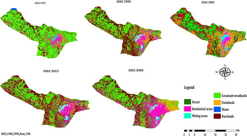
Figure 4. Variation of annual precipitation and monthly maximum consecutive 5-days from 1983 to 2020.

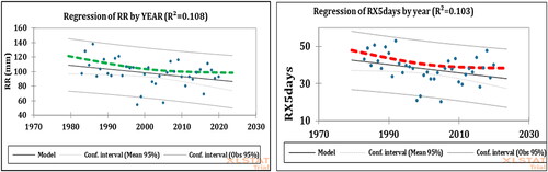
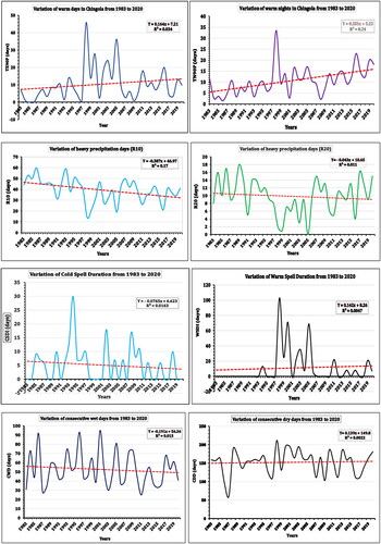
Figure 5. Trend analysis of few climates change detection monitoring indices from 1983 to 2020.

3.1.2. Accuracy assessment

Considering the Cohen Kappa statistic classification scale given by (Landis and Koch 1977), the after post-classification performed in this study lies within the very good range of agreement. The LULC classification’s overall accuracy ranged from 88 to 93 percent, with the lowest accuracy observed from the LULC 1972 classification map and the highest from the 2020 LULC map (see details of Accuracy assessment results in the Appendix (Tables A5–A9)).

Table 9. Summary of land use and land cover structure index and Comprehensive index.

Year	LULC types	Land-use intensity Index (LDI)	Single land use dynamic degree (SLUDI) (%)	Land use and cover rate ($A_i)$	Rate of change (ha/yr)	Comprehensive land use dynamic index (CLUDI)
1972–1992	Forest	−0.04	−7.7	−0.02	−1.9	0.154
	Residential areas	0.03	5.5	0.017	1.7	0.0935
	Mining areas	0.08	15.96	−0.06	6	0.9576
	Savannah woodlands	−0.12	−94.2	−0.0134	1.3	1.262
	Water bodies	0.09	−2.73	−0.015	−1.5	0.041
	Farmlands	−0.01	18.5	0.038	3.8	0.703
	Bare lands	−0.02	−4.62	−0.0011	−5.8	0.0051
CLUDI = 100$\sum {\mathit{SLUDI}}_{}$						322
1992–2001	Forest	−0.03	−5.88	−0.049	−4.9	0.289
	Residential areas	0.06	15.95	0.068	6.8	1.1
	Mining areas	−0.03	−6.72	−0.04	−3.8	0.255
	Savannah woodlands	−0.10	−21.63	−0.035	−3.5	0.757
	Water	0.10	−1.72	−0.03	−2.5	0.043
	Farmlands	−0.01	21.21	0.054	5.4	1.14
	Bare lands	0.01	2.52	0.01	1.0	0.0252
CLUDI = 100$\sum {\mathit{SLUDI}}_{}$						360
2001–2013	Forest	−0.02	−9.2	−0.048	−4.87	1.35
	Residential areas	0.09	37.5	0.0387	3.87	0.227
	Mining areas	0.01	36.7	0.0132	1.32	1.98
	Savannah woodlands	−0.11	−24.78	−0.043	−4.3	0.0942
	Water bodies	−0.06	−4.3	−0.0154	−1.54	1.067
	Farmlands	−0.01	−10.8	−0.0215	−2.2	0.21
	Bare lands	0.09	−59.2	−0.042	−4.2	1.31
CLUDI = 100$\sum {\mathit{SLUDI}}_{}$						623
2013–2020	Forest	−0.011	−4.83	−0.048	−4.87	0.232
	Residential areas	0.045	16.2	0.0387	3.87	0.627
	Mining areas	−0.014	2.73	0.0132	1.32	0.036
	Savannah woodlands	0.008	−23.73	−0.043	−4.3	1.021
	Water bodies	−0.013	−1.13	−0.0154	−1.54	0.0174
	Farmlands	−0.005	−12.81	−0.0215	−2.2	0.275
	Bare lands	−0.011	2.52	−0.042	−4.2	0.11
CLUDI = 100$\sum {\mathit{SLUDI}}_{}$						210

The LULC changed significantly during the study period (1972–2020), with a significant increase in built-up areas and mining areas, and farmlands. Most forested areas have been degraded and converted into savannahs. The increase in farmlands, mining, and built-up occurred at the expense of natural resources, for instance, between 1972 and 1992, forest cover declines from 19,626 ha to 13,465 ha while Savannah woodlands decline from 84,095 ha to 64, 268 ha. During the same period, water bodies declined from 8929.6 ha to 6675 ha while mining areas increased from 5782.5 ha to 18,515 ha along with Built-ups areas that increases from 10,707 ha to 14,987 ha. The observed changes over 48 years, a significant loss of forest cover, from 11.7% in 1972 to 1.8% in 2020. Savannah woodland was found to be the most dominant biome natural resource category, accounting for 50% (84,095 ha) of the total study area in 1972. Its total coverage declined to 22% (36,956 ha) of the total study area in 2020. Water bodies have shrunken steadily from 5.3% (8929.6 ha) in 1972 to 2.1% (3560 ha) of the total study area coverage in 2020, a shrinkage of about 5369.6 ha (Table 6). Savannah woodlands despite being the most dominant biome experienced the greatest loss in area cover of about (−47,139 ha) between 1972 and 2020 (Figures A1 and A2 in the Appendix).

Table 6. Calculated area of the land cover of Chingola in 1972, 1992, 2001, 2013, and 2020.

Classes	1972	%	1992	%	2001	%	2013	%	2020	%
	Area (ha)		Area (ha)		Area (ha)		Area (ha)		Area (ha)
Forest	19,626	11.7	13,465	8.0	8653.8	5.2	4825	2.9	3050	1.8
Builtups	10,707	6.4	14,987	8.9	24,737	14.7	40,635	24.2	48,243	28.7
Mining area	5782.6	3.4	18,515	11.0	13,141	7.8	15,394	9.2	13,067	7.8
Savannah woodlands	84,095	50.1	64,268	38.3	46,878	27.9	27,896	16.6	29,283	17.4
Farmlands	12,881	7.7	27,663	16.5	44,883	26.8	34,685	20.7	32,585	19.4
Water bodies	8929.6	5.3	6675	4.0	5315.2	3.2	4415.7	2.6	3560	2.1
Barelands	25,797	15.4	22,283	13.3	24,172	14.4	39,904	23.8	38,086	22.7
TOTAL	167,818.2	100.0	167,856	100.0	167,780	100.0	167,754.7	100.0	167,874	100.0

3.1.3. Land development intensity and annual growth rate

Table 7 contains the annual growth rate and the land development index per land use category. The result showed that built-ups areas have the highest growth rate per annum (7.3%/year), followed by farmlands (3.18%/year). More details about the land use and land cover conversion between 1972 and 2020 is given in Table A4 in the Appendix.

Table 7. Land use/land cover change development intensity and annual growth rate from 1972 to 2020.

Classes	Change rate/year (1972–1992)	LDI Total	Change rate/year (1992–2001)	LDI Total	Change rate/year (2001–2013)	LDI Total	Change rate/year (2013–2020)	LDI Total	Change rate/year (1972–2020)	LDI total
Forest	−1.72	0.069	−3.97	0.12	−3.68	0.11	−5.25	0.058	−1.75	0.18
Residential areas	1.99	0.06	9.45	0.57	3.87	0.23	2.67	0.120	7.3	1.61
Mining Areas	22	1.76	−3.22	0.096	1.43	−0.04	−6.79	0.095	0.82	0.03
Savannah woodlands	−1.17	0.14	−3.0	0.3	−3.37	0.34	3.27	0.026	−0.98	0.32
Water bodies	−0.53	0.05	6.92	0.69	−1.89	−0.19	−0.86	0.011	−1.25	−0.15
Farmlands	−5.73	0.06	−2.26	0.023	−1.41	0.01	−2.76	0.014	3.18	−0.10
Bare land	−0.72	0.014	1.1	0.011	5.42	0.05	−4.23	0.047	0.18	0.01
TOTAL		2.15		1.81		0.52		0.37		1.90

Table A4. Land use and land cover change transitions between 1972 and 2020.

LULC 2020
	From	To	Barelands	Built-up areas	Farmlands	Forest	Mining areas	Savannah woodlands	Water bodies	Total area (1972)
LULC 1972	Barelands		13,060.7	3550.6	117.9	326.6	1508.4	6125.0	3853.7	28,543.0
	Built-up areas		821.6	7176.0	31.8	64.8	1306.9	1159.9	2010.3	12,571.2
	Farmlands		638.0	3146.5	26.1	18.7	778.8	773.0	1607.5	6988.5
	Forest		475.0	1124.3	1.7	586.4	142.3	3009.5	1248.8	6588.0
	Mining areas		366.9	1177.6	70.4	5.2	1733.9	655.6	467.9	4477.5
	Savannah woodlands		14,846.4	19,963.2	139.8	1603.8	4465.5	46,428.3	15,321.0	102,768.0
	Water bodies		2069.1	193.4	60.7	41.1	95.1	921.1	227.6	3608.0
	Total area (2020)		32,277.7	36,331.6	448.4	2646.6	10,030.9	59,072.3	24,736.8	165,544.4

Values are in hectares.

Accuracy assessment tables of land use/land cover classifications of Chingola district in 1972, 1992, 2001, 2013, and 2020, respectively, in Tables A5–A9.

Table A5. 1972.

	Forest	Built-up areas	Mine areas	Savannah woodlands	water	Farmlands	Bare lands	Total (user)	User's accuracy
Forest	43	0	0	0	0	0	0	43	100%
Built-up areas	0	35	4	0	0	0	0	39	89.7%
Mine areas	0	0	50	0	0	0	0	50	100%
Savannah woodlands	1	0	0	47	0	2	0	50	94%
Water	3	0	0	6	33	0	0	42	78.5%
Farmlands	1	0	0	0	2	38	0	41	90.47%
Barelands	0	0	0	5	0	1	36	42	85.7%
Total (Producer)	48	35	54	58	35	41	36	307	91.2%
Producer’s accuracy	89.6%	100%	92.5 %	81.03%	94.3%	92.7	100%	92.87%
Overall accuracy									91.85%
Kappa statistics									0.90

Table A6. 1992.

	Forest	Built-up areas	Mine areas	Savannah woodlands	Water	Farmlands	Barelands	Total users	User's accuracy
Forest	50	0	0	0	0	0	0	50	100%
Built-up areas	10	39	1	0	0	0	0	50	78%
Mine areas	0	0	50	0	0	0	0	50	100%
Savannah woodlands	0	0	0	49	0	1	0	50	98%
Water	0	0	3	0	47	0	0	50	94%
Farmlands	0	0	0	5	3	42	0	50	84%
Barelands	0	0	0	5	0	4	41	50	82%
Total (Producer)	60	39	54	59	50	47	41	350	90.86%
Producer’s accuracy	83.3%	100 %	92.59 %	83.1%	94%	89.4%	100%	91.77%
Overall accuracy									90.85%
Kappa statistics									0.89

Table A7. 2001.

	Forest	Built-up areas	Mine areas	Savannah woodlands	Water	Farmlands	Bare lands	Total users	User's accuracy
Forest	47	0	0	4	0	0	0	51	92.1%
Built-up areas	0	29	0	0	0	2	0	31	93.5%
Mine areas	0	0	34	0	0	0	0	34	100%
Savannah woodlands	0	0	0	33	0	1	0	34	97%
Water	0	0	3	0	47	0	0	50	94%
Farmlands	0	0	0	1	3	38	0	42	90.4%
Bare lands	0	0	0	5	0	2	61	68	89.7%
Total (Producer)	47	29	37	43	50	43	61	310	93.8%
Producer’s accuracy	100%	100 %	91.89 %	76.74%	94%	88.37%	100%	93%
Overall accuracy									93.2%
Kappa statistics									0.92

3.1.4. Urban sprawl analysis

The Results of human-induced urban sprawl are found in Table 8. The highest human pressure was exerted on savannah woodlands (−0.78), farmlands (0.76), and built-ups areas (0.44) between 1992 and 2001 (0.76). Between 1972 and 1992, agriculture, mining activities, and urban expansion's most important impacts were exerted on Savannah (−0.5) and forests (−0.16) (Table 8).

Table 8. Urban sprawl index (USI).

Classes	1972–1992	1992–2001	2001–2013	2013–2020	1972–2020
USI builtups	0.11	0.44	0.43	0.20	0.27
USI mining areas	0.16	−0.31	0.06	−0.06	0.05
USI Farmlands	0.37	0.76	−0.27	−0.05	0.14
USI Forest	−0.16	−0.21	−0.10	−0.045	−0.12
USI Savannah	−0.50	−0.78	−0.51	0.04	−0.40
USI Water bodies	−0.057	−0.061	−0.024	−0.022	−0.04
USI Barelands	−0.09	0.085	0.42	−0.05	0.09

3.1.5. Land use dynamics

The Land-use dynamic using the Single land-use dynamics and the comprehensive land use dynamic index (CLUDI) in the Chingola district from 1972 to 2020 are shown in Table 9. A negative land use development index was observed for some land use categories such as Forest, Savannah woodlands, and water bodies while built-ups areas, mining areas, farmlands, and bare lands gained in area coverage between 1972 and 2020. Considering the dynamic of change of each land-use class estimated by the single dynamic land use dynamic index (SLUDI), the greatest transformation of land for mining activities occurred between 1972 and 1992, with a land-use development index of 15.96%. From 1992 to 2001, the landscape was transformed by Farmlands (21.21%), built-ups areas (15.95%), while the fastest decline rate occurred in savannah woodlands (−21.63%), followed by mining areas (−6.72%), forest (−5.88%) and water bodies showed the lowest (−1.72%) but a very significant change rate. Nevertheless, the fastest decline in forest cover occurred between 2001 and 2013 with a decline of about (−9.2%), and Savannah woodlands (−94.2%) between 1972 and 1992. It is important to note that the consistent decline in vegetation and increasing pressure on natural resources due to the increasing population have seriously impaired the restoration and conservation efforts. A temporal variation has been observed in LULC, with the highest Comprehensive Land Use dynamic degree over the 48 years of the study period, observed between 2001–2013 (623), followed by (360) observed between 1992–2001, (322) for the period 1972–1992. The lowest value (210) was observed between 2013 and 2020.

3.2. Analysis of the environmental and bioclimatic factors of land cover change intensity

3.2.1. Bioclimatic factors analysis

The temperature (Maxi, mean and mini), precipitation, potential evapotranspiration were analyzed. Precipitation is an important factor for soil and plant growth and useful for the determination of weather patterns regarding early warning of drought and flood (Ficka and Hijmans 2017). Temperature (C3) is useful to classify the weather patterns in combination with precipitation and soil moisture (Ficka and Hijmans, 2017). The analysis showed, a significant changes in the land-use and land cover as well as some natural factors depicting environmental quality through some specific indicators. The analysis of 37 years (1983–2020) of climate variables such as temperature (Maximum, mean, and Minimum), as well rainfall, and PET shows a tremendous change in the bioclimatic conditions of Chingola. The temperature (Maximum, mean, and minimum) has increased for about 0.55 °C, 0.47 °C and 0.45 °C) respectively.

The Analysis of 10 ETCCDMI core Climate Indices, showed that in Chingola the total annual amount of rainfall has declined. Likewise, the analysis showed that rainfall intensity and distribution have significantly decreased. A decrease trend was observed in the annual rainfall with 1986, 1984 and 1992 recorded as the wettest with respectively rainfall amount above normal of 1631.4 mm, 1515.3 mm, and 1433.7 mm respectively. The driest years with a precipitation below normal of 625.1 mm observed in 1998, 661.7 mm in 2005 and 760.3 mm in 1999. A negative trend was observed in the monthly maximum consecutive 5-days precipitation (Rx5days). The highest values of 5 consecutive days in the month with intense rainfall were observed in the years 1992 (282.86 mm), 2015 (216.1 mm) and 1984 (195.7 mm). The Annual count of days when PRCP> =10mm (R10), and the Annual count of days when PRCP> =20mm (R20) also showed a decreasing trend. The peaks in the number of heavy precipitation days (R10) were observed in the years 1986 (60 days), 1993 (59 days) and 1984 (53 days) while the peaks in the number of very heavy precipitation days (R20) were observed in 1989 (18 days), 1986 (17 days) and 2017 (16 days). The consecutive dry days (CDD) have increased during the study period while the Consecutive wet days (CWD) have declined. The years with the highest number of consecutive days were observed in 1998 (212 days), 2000 (196 days), and 1988 (190 days) and the years with the highest number of consecutive wet days were recorded in 2001 (95 days), 1996 (93 days) and 1986 (92 days). The analysis showed that the days (TX90p) and nights (TN90p) are becoming warmer and warmer. The years with the hottest days (percentage of days when TX >90th percentile) were recorded in 1998 (46 days), 2005 (36 days) and 2000 (28 days) while the years with the coldest nights were recorded in 1994 (34 days), 2016 (23 days) and 2019 (20 days). The warm spell duration (WSDI) has increased while the cold spell (CSDI) duration has declined during the study period (1983–2020). The WSDI (highest count of days with at least 6 consecutive days when TX >90th percentile) also pinpoints the hottest years in the time series which were 1998 (103 days), 2000 (71 days) and 2005 (69 days) and coldest years displayed by the CSDI were observed in 1994 (30 days), 2002 (18 days) and 2008 (17 days). However, the highest temperature from 1983 to 2020 was recorded 1994 (39.2 °C) and the lowest was recorded in 1985 (4.08 °C).

The summary statistics on the patterns of Annual total wet-day precipitation (PRCPTOT) and that of the monthly maximum consecutive 5-days precipitation (Rx5days) are found in Tables A1 and A2 in the Appendix.

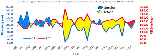
The annual rainfall has decreased by about (−3.25%) while the potential evapotranspiration has increased by 0.04%, giving an Aridity Index (0.60) of (UNEP) and moisture deficit index (−0.42) of Thornthwaite and Mather (1955). Thus, the climate of Chingola can be categorized as dry-subhumid based on the UNEP’s aridity classification and semi-arid according to the United Nations Conference on Desertification aridity classification. However, the analysis classified the Chingola climate type based on the Thornthwaite Moisture Index (−42) as Arid (see TMI climate type classification scheme in Table A3 in the Appendix). Figure 6 exhibits the patterns of rainfall with emphasis on the surplus and deficit in Chingola to pinpoint the degree of dryness or wetness. The analysis showed that 1999, 2000, 2005, and 2017 with the greatest rainfall deficits, with the surplus observed in 1983, 1985, 1989, 1991, 1993, and 2009.

Figure 6. Patterns of rainfall deficit and surplus observed in Chingola from 1983 to 2020.

3.2.2. Environmental factors analysis

This study strives to understand the patterns, magnitude and trend of land degradation and subsequent changes in the environmental factors in Chingola. The analysis showed a decrease in vegetation greenness translating to the depletion of natural vegetation during the study period with 85% explained by the interannual variation and 15% by other factors. A pixel value derived from this NDVI analysis below 0.2 is considered bare land. When (0.2 ≤ NDVI≤ 0.5), it stands for a mixture of bare land and vegetation, and NDVI > 0.5, should be considered a fully vegetated area as recommended by many scholars (Sobrino et al. 2004, 2008; Skovic 2014; Yu, 2014b; Li and Jiang 2018). Sobrino et al. (2004) recommended in the global situation a threshold value of 0.5 for the maximum of NDVI and 0.2 for the minimum value of NDVI (NDVI_min). The same negative trend was observed for NDWI between 1972 and 2020, with the lowest value observed in 2001 and 56% of the variation explained by the interannual variation and 44% by other factors. Likewise, similar negative trends were observed for soil salinity (NDSI) and vegetation moisture content (NDMI).

The result showed a decreasing trend in NDVI, NDWI, NDMI, and NDSI between 1972 and 2020 (see Tables 10 and 11, and the Figures 7–10).

Figure 7. Spatio-temporal variation of NDVI and NDWI in Chingola from 1972 to 2020.

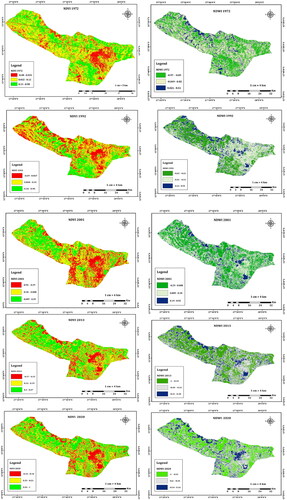
Figure 8. Annual variation of NDVI and NDWI (Max, Mean, and Min) from 1972 to 2020.

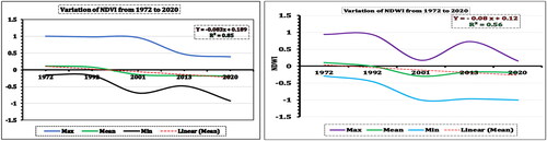
Figure 9. Spatio-temporal variation of NDSI and NDMI in Chingola from 1972 to 2020.

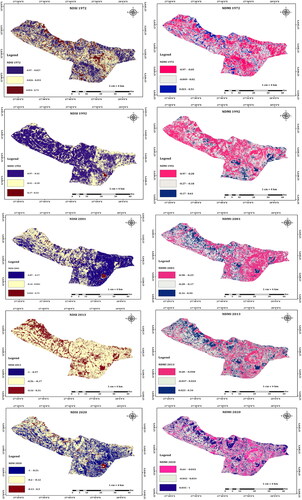
Figure 10. Annual variation of NDSI and NDMI (Max, Mean and Min) from 1972 to 2020.

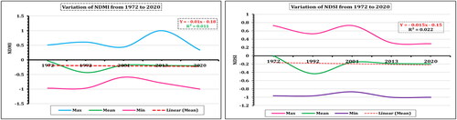
Table 10. Variation of environmental factors.

	1972	1992	2001	2013	2020
Average environmental indices
NDVI	0.18	0.17	−0.14	0.09	0.11
NDWI	0.11	0.02	−0.30	−0.17	−0.19
NDSI	−0.002	−0.43	−0.158	−0.189	−0.196
NDMI	−0.033	−0.43	−0.18	−0.19	−0.20

Table A1. Summary statistics of annual precipitation regression analysis.

Variable	Observations	Obs. with missing data	Obs. without missing data	Minimum	Maximum	Mean	Std. deviation
RR	38	0	38	53.8	137.453	97.64	17.54
The goodness of fit statistics (RR)
Observations	38	MSE	282.257
DF	36	RMSE	16.8
R²	0.108	MAPE	14.356
Adjusted R²	0.083	DW	1.798

Table A2. Summary statistics of RX5days.

Variable	Observations	Obs. with missing data	Obs. without missing data	Minimum	Maximum	Mean	Std. deviation
RX5days	38	0	38	20.1	52.76	37.	7.57
The goodness of fit statistics (RX5days)
Observations	38	MSE	52.91
DF	36	RMSE	7.27
R²	0.108	MAPE	16.1
Adjusted R²	0.078	DW	1.798

4. Discussion

4.1. Magnitude, intensity, and dynamics of change between land use and land cover categories from 1972 to 2020

4.1.1. Changes in magnitude of LULC from 1972 to 2020

The results showed substantial changes in LULC in Chingola District, between 1972 and 2020. There is a territorial polarization of development, with most of it concentrated in the city’s Center-west, where jobs and adequate infrastructures are available and expanding to the periphery and along the major highways. The results were like the research carried out by (Sakuwaha 2017) in the Luyanshia District of Copperbelt. Sakuwaha found that the growth of Luyanshia city was concentrated around the mining areas and less in the peripheries of the district. Similarly, Thapa and Murayama (2011) studied urban growth in the Kathmandu metropolitan region, Nepal, and reported that cities expand from areas with adequate infrastructure toward the city outskirts, into open lands with perceived suitable development potential. The study has shown that the main drivers associated with the dynamic and patterns of LULC in the Chingola district are population growth, infrastructure development, and expansion in agriculture, and mining activities. Environmental sustainability and sustainable urban development can be improved through informed land-use planning (Enoguanbhor et al. 2019). Uncoordinated, unenforced, or non-existent land use planning may result in haphazard development (Yin 2012) and excess deterioration of the built and natural environments. In less developed countries (particularly in Sub-Saharan Africa), rapid urban expansion and growth of informal settlements challenge current efforts for sustainable land use planning (UN-Habitat 2008).

Over the study period, a significant increase was observed in farmland, built-up, and mining areas. The mining areas in Chingola increased consistently by about 1.4% over the study period (1972–2020), with the highest land development urban sprawl index (7.6) observed between 1972 and 1992. However, a slight decline of about (−3.2%) between 1992 and 2001. The impacts of mining in the study area included but were not limited to large open pits, deep shafts, a large volume of overburden materials and mine waste, tailings storages facilities, air pollution deriving from the smelting plants, siltation of rivers, polluted rivers and lands large volume of water extracted from the underground mine, which is one of the wettest in the world. This observation is common in almost all the mining districts in the Copperbelt province of Zambia (Limpitlaw 2001; Lindahl 2014). In Chingola, mining activities have not only altered the landscape and vegetation but have also accelerated environmental degradation. For instance, a substantial increase in farmlands was observed between 1992 and 2001, coinciding with a decrease in mining areas. A review of the literature revealed that major environmental, institutional, and political changes happened in Zambia during the same period (1992 to 2001). Some of these policies included but were not limited to the Structural Adjustment Programme (SAP), implemented by the Zambian Government between 1990 and 1995 (Handavu et al. 2019), and the changes in mine policies that led to a relative slowdown in mining activities. During this same period, the urban population declined from 39% in 1990 to 35% in 2000. The rural population increased by 1,657,580 inhabitants while the urban population increased by not much than 428,980 inhabitants with an annual average growth rate of 3.0% and 1.3% respectively (CSO 1990a, 1990b, 2000, 2011; Crankshaw and Borel Saladin 2019). Eventhough there is no clear scientific evidences explaining the connection between the slowdown in mining activities and decline in urban population and increase in the rural population, it is believe that this slowdown might have triggered the migration of many urban dwellers to rural areas to seek for alternative livelihoods or activities such as agriculture and chalcoal burning, given the increase in farmlands and decline in forest and water resources observed this period.

Moreover, the analysis of 10 Climate change detection indicators revealed that the driest and hottest years in 1983–2020 timeseries were found within the period 1992 to 2001. For example, 1998 was the year with the lowest rainfall amount (625.1 mm), the highest consecutive dry days in 1998 (212 days), 2000 (196 days) and 2001 (195 days). Other indicators such as WSDI found 1998 (103 days), the years the higher of hot days TX90P (46 days) and higher number hot nights (34 days). The combination of these factors mounted a huge consequence on the ecosystem. Our findings are in line with the studies done by Capitanio et al. (2016) and Pascucci et al. (2013), which ascertained that LULC changes can be influenced by policy implementation. Nevertheless, agricultural activities and mining activities can both affect negatively the environment. Ticci and Escoba (2015) and Andersson (2017) estimated the impact of mining on the productivity of agriculture and proposed solutions to channel these impacts to maximize benefits that can contribute to sustainable development. However, there is still a long debate on this problem as scholars’ views are still divergent. Ticci and Escoba (2015) found that mining companies in Peru have no statistically significant impact on agricultural production and prices. Andersson (2017) found that agricultural production did not decrease with the proximity to the mining areas. In contrast, Aragon (2015) estimated that gold mining in Ghana reduces the productivity of nearby farming activities due to environmental damage. A negative impact of coal mining on agricultural productivity has also been found by Mishra and Pujari (2008) in the Indian state of Orissa. Our findings resonate with previous studies done in the same Copperbelt Province by (Mines 2007; Mususa 2014; Sakuwaha 2017), in West Africa by Hermann (2020) who found that land degradation appeared to be threefold higher in the vicinity of settlements and farmlands compared to others, between 1975–2013 and Mensah et al. (2017), discovered that most farmers who lose their farmlands due to mining activities encroached into the forest reserves which resulted in the conversion and depletion of forest cover areas from 75.54 km² in 2002 to 27.76 km² in 2015.

The status of surface water and soil moisture content, using NDWI and NDMI during the study period, showed a decreasing trend in Chingola. This shrinkage can be explained by the opening of farmlands and built-up and mining areas expansion. Our findings are in line with (Limpitlaw 2001; Ashraf et al. 2009; Subramani and Vishnumanoj 2014) who identified deforestation and forest degradation as the main drivers, affecting water catchments and hydrology.

In the coastal city of Jiangsu, China, Li et al. (2013) reported that water bodies shrank the most during the period when agricultural activities and deforestation intensified. In Ghana, Hilson and Nyame (2006) found a link between increased deforestation, mining expansion, and shrinkage of water resources. The study observed a significant loss of forest cover in Chingola, from 1972 to 2020, decreasing from 19,626.84 ha in 1972 to 3050 ha, with an annual rate of deforestation of about (−1.75%yrs⁻¹). A similar observation was made by Limpitlaw (2001), in Kitwe, a neighboring mining District of Chingola. The annual deforestation rate in Zambia estimated to be approximately 276,021 ha per annum, making it one of Africa's highest annual deforestation rates (ILUA 2017). This figure is relatively higher in Nigeria, where the deforestation rate is around 350,000–400,000 hectares per annum (Ladipo 2010). This rate of deforestation greatly contributes to major global concerns such as increasing concentrations of carbon dioxide (CO₂) in the atmosphere, loss of biological diversity, conversion and fragmentation of natural vegetation areas, and accelerated emission of greenhouse gases (Steffen et al. 2006). Also, because forests store carbon and reduce the impacts of drought and flooding, the loss of forests reduces carbon sequestration and climate resilience (Hirsh-Pearson et al. 2022). Most of the reserve forests in Chingola have been completely depleted and absorbed by urban expansion. The analysis using remotely sensed data and the visit of all classified forest reserves (Luano Forest reserve No. 12, Chingola Forest Reserve No. 43, Lushishi Forest reserve No. 11, Lamba Protected Forest area) in the district, showed that some of these forests have disappeared completely, absorbed by the urban expansion (Chingola forest reserve and Luano forest reserve) and some highly encroached by anthropogenic activities (Lushishi Forest Reserve No. 11 and the Kirila forest reserve adjacent to the hippo pool). By the year 2003, Mwila (2003) alerted that the Luano national forest in Chingola was highly encroached by anthropogenic activities. The local people dwelling in the area stated that, they do not view the area as a forest but rather as an agricultural area. Our study found that the alert was not taken seriously leading to the total depletion of the forest reserve among others. Among the factors depleting the forest, there are agriculture, charcoal production, wildfire, settlement, and poverty.

As early as 1972, Maxwell (1972) indicated that the encroachment of the Luano catchment area will disturb the hydrological cycle. Yemshanov et al. (2015), demonstrated that forested lands located near existing urban and agricultural areas are most at risk of being converted to cropland or human settlement. Land use and land cover change through land conversion to man-made infrastructures affect the local ecosystem through altering water and air quality, the nutrient cycles, and degrading a large portion of arable lands by paving them with impermeable materials such as asphalt or concrete (Environment and Climate Change Canada 2021).

Nevertheless, the vegetation in Chingola is mainly composed of miombo woodlands, which have been found to recover rapidly from disturbances caused by human activities in Zambia (Boaler and Sciwale 1966; Luoga et al. 2004; Syampungani 2008; Chirwa et al. 2014). Moreover, a study by Zhen (2019) demonstrated that with a very good policy and technology, it is possible to curb land degradation and restore ecologically vulnerable regions. For instance, returning farmland to forest or grasslands through artificial afforestation. However, the major constraints and threats to reforestation initiatives are the growing insecurity in the land tenure system and growing scarcity of arable lands for growing subsistence crops, hindering long-term investment in on-farm tree planting. All these factors are exacerbated by population growth and the need to secure lands for future infrastructure development (McMillan et al. 1993; Nebie and West 2019).

4.1.2. Land-use intensity and dynamic degree

Considering Jagadeesh et al. (2015), the CLUDD classification scheme and having seven land use and cover classes, the upper limit of the Comprehensive Land Use Dynamic Degree (CLUDD) was set at 700, which equates to the highest combined impact from both natural and human activities and thus indicates the degree of degradation of the biophysical environment of the study area. The highest LULC Comprehensive Index (366), observed between 2001 and 2013, can be explained by the boom in the socio-economic activities that followed my privatization in Zambia in 1997. This privatization regime attracted massive direct investment in the mining sector and indirect investment in other economic activities such as farming and businesses; subsequent economic growth led to a rapid increase in built-up and the opening of new mining areas.

4.1.3. Urban sprawl implications on the environment in Chingola

Urban sprawl is a complex phenomenon, which goes beyond average population density. Its different dimensions reflect how population density is distributed across urban space and how fragmented urban land is (OECD 2018). It is important to understand the extent to which Chingola has grown from 1972 to 2020 as this is important for policymakers, urban planners, and decision-makers. Urban sprawl has implications on the increase of the per-user costs of providing public services of primary importance (water supply, sanitation, electricity, public transport, and waste management) that are key for the well-being of the population. The field survey showed a regional disparity and imbalance in terms of development with most public services concentrated and only available within Chingola town near the mine, and the administration, while the other wards (Mutenda on the west and Musenga on the southeast) at the far end of the district are left without and underdeveloped.

The analysis of urban sprawl in Chingola using the urban sprawl index showed the magnitude of human activity in each land use category. Forest cover, water bodies, and savannah woodlands have all been stressed by anthropogenic activities. The trend of forest and wetlands degradation, if not curb, will alter their ecological functions and their ability to cool the micro-climate, filter freshwater from heavy metals, and provide habitat for many terrestrial and aquatic species.

With Chingola’s population projected to continue its unabated increase over the next decades (DPU 2019), intensification of land cover change is expected. Taking the past as an indicator of the future, the observed patterns of change and persistence give an idea of what types of future changes might occur, and which areas should be prioritized for policy implementation. Several studies have also revealed the role of agriculture in changing the vegetation pattern thereby altering the characteristics of local meteorological parameters (Niyogi et al. 2010; Rahimian et al. 2021). Urban containment policies and initiatives that encourage agricultural intensification are needed to counteract the tendencies of agriculture to spatially expand and further encroach into savannah woodlands and forest areas. Draconian measures should be taken to limit slash-and-burn farming activities on the edge of water bodies. The teleconnection between land use and land cover change intensification through urban sprawl and population growth and its implications on the bioclimatic and environmental factors can never be over-emphasized. Land cover trajectories and urban expansion determine land surface fluxes at local and regional scales, amplifying aridity and global warming. Curbing urban sprawl requires promoting socially desirable levels of population density and reducing urban fragmentation through urban containment policies. It also requires reforming land-use regulations and property taxation which is key to achieving more sustainable urban development patterns. Putting Boundaries to urban development may be effective in protecting forestland on the outskirts of the city of Chingola and others cities in Zambia and designated open spaces of environmental importance. Existing urban growth boundaries, buffer zones, and greenbelts should be periodically reviewed and reformed.

4.2. Environmental and bioclimatic factors analysis in relation to land degradation

4.2.1. Implications of changes in the bioclimatic factors on the socioeconomic sectors

The computed slope value of total annual rainfall was found negative, implying a decrease of rainfall over three decades of about (−3.25%). This can be explained by the increase in temperature and potential evapotranspiration transforming the district to a dry-subhumid area with a moisture deficit standing at −0.42. Moreover, our analysis of 10 climate change detection indices showed that the district is becoming warmer (nights and days) and drier (increase in consecutive dry days and decline in the consecutive wet days). The rainfall intensity has also declined significantly (lesser days of heavy rainfall). Some effects of heatwaves include but are not limited to effects of heatwaves, heat rash, heath cramps (occurring when body temperature reached T = 35 °C, with an increase in heart rate, loss of water and salts from the muscles), heat exhaustion (occurring when body temperature reached, T = 40 °C, follow by increase heart rate, and sweating), and heat stroke (increase in the body temperature to T ≥ 45 °C, dry skin, swooning, damage of certain organs, and possible death) (Tong et al. 2010; Coumou and Rahmstorf 2012; Perkins and Alexander 2013; Ncongwane 2015).

These results are consistent with the findings of Chabala et al. (2013) and Lubinga et al. 2019) who found an increasing trend in temperature in all selected areas in Zambia. However, there is still a clear geographical disparities in terms of impacts of climate change across the continent. If the amount of rainfall received per annum in most southern African countries including Zambia is decreasing, recent studies on the Western African Sahel showed that the amplitude and frequency of heavy rainfall events have increased significantly (Taylor et al. 2017; Salack et al. 2018; Bichet & Diedhiou, 2018).

Nevertheless, a decline in rainfall amount and an increase in dry days and temperature pose a significant risk of soil moisture stress, which ultimately results in crop failure and food insecurity (Hulme et al. 2001; Seleshi and Zanke 2004; Alemayehu and Bewkt 2015, Zhao et al. 2020). A study by Nebie and West (2019), described population pressure and deforestation as the major causes of the severe famines in the Sahel in the 1970s and 1980s. Xing (2015) and Yu (2014a) ascertained that a decrease of rainfall below-normal under a rising temperature provide adequate condition to trigger frequent and severe meteorological drought.

Consequently, the struggle of the small-scale farmers to obtain surface and ground water for their crops, livestock and household consumption is going to worsen with the current rate of environmental degradation, considering that 98% of Zambia's agricultural land is rain-fed (FAO/IFC 2014). However, if it is obvious and generally accepted by many studies that climate change affects the agricultural sector, not much research has been done in Zambia regarding climate change and its effect on crop yields, particularly under a consistent increase in temperature and decrease in rainfall (Lubinga et al. 2019). The few undertaken in the country used low-resolution data (Lubinga et al. 2019), generalizing their findings to different agro-ecological zones, thereby providing fewer insights to both policy makers and farmers (Kachulu 2018; Lubinga et al. 2019). Lubinga et al. (2019) found that variation in the yields of maize was much more influenced by the increase in minimum temperature and soil management practices than other climatic variables, including El Nino and La Nina in Mpongwe, a district in the same agroecological zone III as Chingola district on the Copperbelt province, Zambia. Iizumi et al. (2014) ascertained that with supplementary irrigation, the effect of El Nino on maize yield can be mitigated. However, considering the level of income, this option will be limited to the majority of the population living below the poverty line.

The changing microclimate in Chingola can be due to the changes that have occurred at global levels, but also in the land use and land cover, replacing some surface parameters such as forest, grasslands, wetlands, and water bodies with artificial features (farmlands, mining areas, built-ups), resulting in increased evaporation and evapotranspiration and shrinkage of surface water. Moreover, the urban growth made with buildings and infrastructures most of which are made with low albedo materials, with high thermal inertia, and the potential of absorbing and storing the heat received from insolation has also played an important role in the increase of air temperature and urban heat islands over the city Centre. Consequently, these factors will put more pressure on the provision of social services and economic activities such as health, agriculture, livestock, and energy in the nearest future. In Senegal, West Africa, (Faye 2017) found that decrease in rainfall and increase temperature affected the agricultural sector in terms of changes in agricultural commodity prices, production structure, and livestock production capacity. A study by Karaca et al. (2002), ascertained that exposure to elevated ambient temperature has a greater impact on semen quality, decreasing fertility in poultry, rabbits, horses, and male birds. These factors trigger an influx of migration from rural to urban areas, with severe implications on measures of well-being such as housing, water, and energy consumption specifically on household air conditioning and human health. The observed trend if maintained can lead to increased risks of dehydration, hyperthermia, and heat stroke mainly affecting the elderly and infants (Kovats and Hajat 2008; Smargiassi et al. 2009).

4.2.2. Environmental factors analysis

Remote sensing also can map and monitor changes in surface conditions, which are not related to a direct change in land cover or land use, most notably that vegetation condition. Trends in the normalized difference vegetation index (NDVI) or other similar indices (NDWI, NDMI, NDSI are often used as a proxy measure of vegetation condition (Al-Bakri and Taylor 2003) and for analysis of the impact of drought (Kourouma et al. 2021). Based on the vegetation indices used for monitoring environmental health conditions (NDVI, NDWI, NDMI, NDSI), through the detection of the presence and absence of vegetation, soil moisture, soil quality, and surface water. The high value of each index indicates the presence of vegetation, moisture, and water, while the low value indicates the absence thereof. A decreasing trend was observed in the average of each indicator. The decrease can be explained by the increase in agricultural activities, expansion of mining, and human settlement that have altered the areas of forest, savannah woodlands, and water bodies.

NDVI value ranges from −0.15 to 1 in 1972, to −0.92 to 0.39 in 2020. A value of NDVI above 0.5 indicates a fully vegetated area and below 0.2 to −1 stands for bare lands and water bodies. NDWI ranges from −0.29 to 0.94 in 1972, to −1 to 0.16 in 2020. A positive value] 0.5, 1] signifies the presence of extensive deep-water bodies, while NDWI ranging from] 0.2 to −1] denotes vegetation covers (Xu 2006; Chowdary et al. 2008; Huang et al. 2009). NDMI ranges between −0.97 to 0.51 in 1972, −1 to 0.34 in 2020. All these factors showed a decline in vegetation covers, surface water availability, and soil moisture, denoting the extent to which the local ecosystem is becoming vulnerable. However, the observed decrease in soil salinity (NDSI) is a good signal for agricultural activities, which might also be explained by the decrease in prolonged waterlogged conditions. Environmental factors such as (NDVI), NDWI, NDSI, and NDMI are among other natural factors that have been widely used as effective indicators to analyze land degradation (Lu et al. 2007; Abdul-Qadir and Benni 2010; Aldakheel 2011; Allbed and Kumar 2013; Nguyen et al. 2016; Ficka and Hijmans 2017; Goigoi et al. 2019; Nguyen and Liou 2019; Kourouma et al. 2021). Analysis of these environmental factors for respectively vegetation cover and greenness, surface water availability, soil moisture, and soil salinity all showed a declining trend over the study period. A decline in NDVI implies greater ecological vulnerability, given its important role in maintaining a good eco-environment and cooling heat island effect. A study was done in Mongolia, China by Ma et al. (2017) revealed that unreasonable exploitation of mineral resources, decreasing precipitation, and temperature are key factors that exacerbate land degradation. It is thus, important to monitor soil moisture as it is vitally important in controlling the exchange of water and heat energy between land surface and atmosphere through evapotranspiration. NDSI acts as a key variable to define flood control, soil erosion, and slope failure (Moran 2009). NDVI and NDWI as having been proved by previous studies here droughts (Gao 1996; Anyamba and Tucker 2005, 2012; Chen et al. 2005) are very useful for detecting and investigating drought effects on vegetation cover in the case of agriculture. Mishra and Singh (2010) argue that NDWI may be a more sensitive indicator than NDVI for drought monitoring, but its developer (Gao 1996) emphasized that the index is: ‘complementary to, not a substitute for NDVI’. Yengoh et al. found NDVI very effective in developing famine early warnings systems, such as FEWS NET, an operational system for data dissemination related to global food production and availability. This system rigorously tested the ability of NDVI to detect areas of imminent food shortages (Hutchinson 1991; Quarmby et al. 1993; Kourouma et al. 2021). A study by Yengoh and Ardö et al. (2014) and Eze et al. (2020) found that NDVI combination with relevant climate data has a very strong potential for forecasting crop failure. This could help decision-makers in understanding the hydrological patterns of the existing watersheds, allowing planners to develop policies that minimize the negative effects of LULC changes and the potential occurrence of hydrological drought, which could be detrimental to the agricultural as well as the mining sector. Considering the importance of natural vegetation, water resource, and wetlands, and the observed decline, the study recommends a watershed approach that is participative, spatially focused, and based on reliable science and data. The application of NDVI, NDWI, NDMI, and NDSI in this study has shown their suitability for detecting changes in a mining environment. Nevertheless, there is a need to regulate farming activities and the establishment of settlements on the edge of water bodies, wetlands, and forest reserves.

4.3. Preventive and mitigation measures to avoid future undesirable impacts of land use and land cover change

Rapid urbanization, population growth and diverse anthropogenic activities are transforming urban landscapes mounting the pressure on housing, health facilities, water supply and sewerage services, solid waste management, transport services, security, energy supply and challenging current efforts of sustainable land use planning and environmental sustainability (UN-Habitat 2008; Seto et al. 2012; Cobbinah and Darkwah 2016, 2017). Providing science-based solutions through determining the pace and magnitude of land use and land cover change, can support policymakers for future development and action plans (Mazeka et al. 2022). In African countries’ economies which are mostly resource-based, the dynamics and intensity at which the landscapes of cities are transformed are shaped by the governance system, the chosen pathways of development (shared socio-economic pathways, overshoot/non-overshoot, mitigation, or adaptation) (Heynen et al. 2006), population growth and human settlements expansion (Iqbal et al. 2013).

Cities’ ability to address key environmental, economic, and social challenges, such as climate change, regional imbalances, access to affordable housing, water, and sanitation facilities, will determine how they develop in the years ahead. This study despite the substantial urban growth found discrepancies and regional imbalances in terms of development in Chingola.

Consequently, consistent and focused policy initiatives at all levels of government are urgently needed to steer urban development toward more sustainable paths, which will be critical for attaining the Paris Agreement and the UN Sustainable Development Goals. To control urban sprawl and minimize land cover fragmentation, the government should consider modifying land-use regulations, urban containment policies, and property taxation, as well as establishing greenbelt or buffer zones to conserve the remnant forestlands on the edges of the district. Practically, the government should prevent the establishment of settlement areas near the forest reserves and agricultural lands to lower the urbanization pressure.

The government should form a Public-Private-Partnership (PPP) with the mining industry to meet their corporate social responsibilities as well as in development planning, supporting the government in constructing roads, public transportation, water, and sanitation in the sprawling and underdeveloped areas of the district where they dont’ necessarily operated. This will allow development and benefits from the mines to be distributed more fairly. The regional and municipal planning boards should not be ‘planning for the people’, but rather ‘planning with the people’, by incorporating citizens’ perspectives and efforts toward future development in government proposal for urban planning and local development initiatives.

Our study discovered that the main causes of the deforestation and degradation of natural resources are the lack of monitoring by the forestry department. Chingola forestry department is severely understaffed and lacking logistical capacity to conduct consistent and regular monitoring of the forest reserves. Recruiting more personnel, providing logistics, and building the capacity of the workers on the current advanced tools for monitoring natural resources such as remote sensing and GIS would increase their effectiveness and efficiency. There is a need to also reform the existent Joint Forest Management strategies with more sustainable management strategies, complemented by stricter regulations on conservation such as urban containment policies and land use taxation.

Moreover, it is noteworthy to keep in mind that African cities' demographic change will be one of the highest worldwide, which will expose the urban population to significant natural hazards such floods, drought and heat in the upcoming decades (Asefi-Najafabady et al. 2018; United Nations 2018). The occurrence and magnitude of these hazards demand more climate-smart strategies of adaptation. For instance, the sustainability of livestock productivity in face of climate change can be improved by implementing new practices and strategies (genetic approaches for breeds resilient to heat stress). Technological adaptation strategies using stress-tolerant crop varieties, irrigation, artificial intelligence for advanced crop monitoring could sustain the agriculture sector. In the sector of transportation government can choose more climate resilient materials for constructing infrastructure such as roads and Railway systems (using high grade heat-resistant asphalt and the use of concrete instead of wood for constructing train track).

The study’s recommendations are valid and applicable to all other districts in Zambia’s agroecological zone III, and if considered have the potential to make a significant contribution to addressing the challenges of tackling poverty (SDG1), help the local government on where to concentrate its effort in achieving food security (SDG2), understanding the current trend and status of environmental degradation and how maladaptation and inactiveness will mount pressure on the energy supply that highly depends on hydroelectricity (SDG7). Parkes et al. (2019) estimated Africa’s cost of energy-intensive cooling systems to 51 billion USD and 487 billion USD by 2035 and 2075 respectively, in the continent where only 44.5% of the sub-Saharan population has access to electricity. As a result, an increase in energy costs due to increasing stress on the water resources would likely lower energy access and its affordability for people with moderate income.

Local government need to proactively plan and move towards revisiting the building codes and settlements regulations. Recommending sustainable cooling solutions for building and roofing materials (cool roofs and green roofs) could help residents contribute towards a more resilient city (SDG11). More efforts should be put on revising the current Paris Agreement’s roadmap and milestones (SDG13). It is worth noting that achieving these objectives are critical to maintaining peace on a local, national, and global scale (SDG16).

Consequently, this study advocates for more multidisciplinary research and collaboration, as well as increased commitment from policymakers and decision-makers at all levels, as well as better policy development and implementation.

5. Limitations of study

This research presented the current state of knowledge about the processes of land use and land cover change, urban sprawl, and its implications on the environmental and bioclimatic factors. Like any other research, it has limitations that would have to be overcome, given the ability to formulate conclusions more broadly. One of the limitations of this study is related to the resolution of the satellite image used (30 × 30) meters for Landsat 5 TM, Landsat 7 TM + and Landsat 8 OLI/TIRS and (60 × 60) meters for Landsat MSS 1. A study of urban sprawl for instance demands small grids and high-resolution satellite imagery. The climate changes detection indicators used in this study as bioclimatic factors derived from the Ndola meteorological station within the same agroecological zone III and within less than 100 km radius. However, although, this station depicts the climatic condition in Chingola, the results could have been more accurate if the data was complemented by satellite climate data such as The Climate Hazards Group InfraRed Precipitation with Station data (CHIRPS) products which could help to extract more stations points. Nevertheless, future research directions should consider these limitations. More studies are needed to understand whether the current urban expansion in Chingola as well as in other parts of Zambia is solely caused by economic growth? by rural-urban migration? by the natural growth of the urban population? by the boom in mining activities and increasing regional demands for natural resources? by the decline of urban mortality rates and improvement of the social welfares and food supply? or by the combination of two or several of these factors.

6. Conclusion

This study assessed LULC dynamics and intensity over the period 1972–2020 using land-use indices and explore the drivers of change. Although other similar studies have been carried out, this research introduces the first attempt to make use of tools available in GIS and remote sensing and as such, it has provided consistent information to fill the existing information gap on land-use and land cover dynamics in Chingola and implications on bioclimatic and environmental factors. It serves as a benchmark for monitoring forest, urban expansion, and climate change and has proposed solutions to manage urban sprawl, expansion in agricultural and mining areas, and most importantly natural resources. The analysis shows that development in Chingola is polarized around mining areas and major roads. Moreover, the analysis shows that from 1972 to 2020, a steady decline in forest cover was observed, and existing policies, regulations, and management systems have failed to restore the forest. On the contrary, most forest reserves are being alarmingly encroached upon and the mine reclamation efforts appear to be relatively limited and inefficient in repairing the environmental damage.

This study used a holistic indicator-based approach in assessing the state and implications of land use and land cover change in terms of urban growth, changes in the bioclimatic and environmental factors, and at the same time provide recommendations to guide cities hosting mining industries toward inclusive and green growth. The study found environmental factors such as (NDVI, NDWI, NDMI, and NDSI) suitable to assess changes in environmental conditions in the mining areas.

More research into how land cover changes affect streamflow, and its components is needed considering the reported shrinkage of water bodies (surface water and groundwater flow). If the current trend is maintained, Chingola will face a high risk of agricultural, meteorological, and hydrological drought. The local government should consider building water storage facilities and protecting the edges of the existing water bodies. Further urban-related studies with socio-economic effects are needed in Zambia for a more in-depth understanding of the dynamics of urbanization and population, which could help to better plan development sectors and address effectively the provision of social services.

Authors’ contribution statement

Jean Moussa Kourouma: Conceptualization, Methodology, Data curation, Analysis, Writing-Reviewing, and Editing. Darius Phiri: Data curation, Writing-Reviewing Original draft. Andrew T. Hudak: Writing-Reviewing and Editing. Stephen Syampungani: Writing-Reviewing. All authors contributed to the editing and reviewing of the manuscript.

Disclosure statement

No potential conflict of interest was reported by the authors.

Data availability statement

The data and materials that support the findings of this study are freely available from the corresponding author [J.M. Kourouma] and can be shared upon reasonable request.

Additional information

Funding

The World Bank financially supported this research through the African Centre of Excellence on Sustainable Mining (ACESM) Scholarship program of Copperbelt University.

Appendix

Figure A1. Area change intensity heatmap for land use and land cover classes between 1972 and 2020.

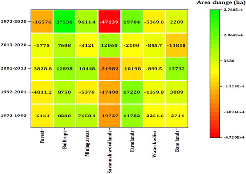
Figure A2. LULC areas change intensity analysis for 1972–2020.

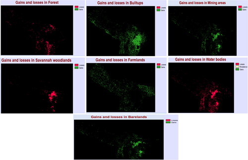
Table A8. 2013.

	Forest	Built-up areas	Mine areas	Savannah woodlands	Water	Farmlands	Barelands	Total users	User's accuracy
Forest	40	0	0	3	0	7	0	50	80%
Built-up areas	0	38	0	4	0	2	0	44	86.36%
Mine areas	0	1	34	1	0	2	0	38	91.89 %
Savannah woodlands	0	0	1	53	0	0	0	54	75.7%
Water	0	0	1	1	36	0	0	38	92.3%
Farmlands	0	0	1	3	3	29	3	39	67.4%
Barelands	0	0	0	5	0	3	72	80	96 %
Total (Producer)	40	39	37	70	39	43	75	343	84.2%
Producer’s accuracy	100%	97.4 %	91.9 %	75.7%	92.3%	67.4%	96%	88.7%
Overall accuracy									88.04%
Kappa statistics									0.86

Table A9. 2020.

	Forest	Built-up areas	Mining areas	Savannah woodlands	Water	Farmlands	Barelands	Total (user)	User's accuracy
Forest	56	0		0	0	0	0	56	100%
Built-up areas	0	53	1	2	2	0	0	58	91.37
Mining areas	0	0	37	4	1	1	1	44	84.1%
Savannah woodlands	0	0	0	51	0	0	0	51	100%
Water	0	0	0	0	47	0	0	47	100%
Farmlands	1	0	0	1	5	56	3	66	84.84%
Bare lands	1	0	0	0	14	0	70	85	87.1%
Total (Producer)	58	53	38	58	69	57	74	407	92.5%
Producer’s accuracy	96.55%	100%	97.36	87.9%	68.1%	98.2%	94.6%	91.8%
Overall accuracy									90.9%
Kappa statistics									0.89

References

- Abdul-Qadir AM, Benni TJ. 2010. Monitoring and evaluation of soil salinity term of spectral response using Landsat images and GIS in Mesopotamian plain Iraq. J Desert Stud. 2:19–32.
- Ahmed HH, Andrianasolo H. 1997. Comparative assessment multisensor data for suitability in study of the soil salinity using remote sensing and GIS in the Fordwah Irrigation Division. IEEE International Conference on Geoscience and Remote Sensing, Singapore, 3–8 August, p. 1627–1629.
- Akinyemi, FO, Pontius Jr, RG, Braimoh AK. 2017. Land change dynamics: insights from Intensity Analysis applied to an African emerging city. J Spat Sci. 62(1):69–83.
- Al-Bakri JT, Taylor JC. 2003. Application of NOAA AVHRR for monitoring vegetation conditions and biomass in Jordan. J Arid Environ. 54(3):579–593.
- Aldakheel YY. 2011. Assessing NDVI spatial pattern as related to irrigation and soil salinity management in Al Hassa Oasis, Saudi Arabia. J Indian Soc Remote Sens. 39(2):171–180.
- Alemayehu A, Bewkt W. 2015. Local climate variability and crop production in the central highlands of Ethiopia. Addis Ababa, Ethiopia: Department of Geography & Environmental Studies, Addis Ababa University.
- Allbed A, Kumar L. 2013. Soil salinity mapping and monitoring in arid and semiarid regions using remote sensing technology: a review. ARS. 02(04):373–385.
- Amin A, Fazal S. 2012. Quantification of land transformation using remote sensing and GIS techniques. AJGIS. 1(2):17–28.
- Andersson M, Hall O, Olen N, Tolonen A. 2017. Does large-scale gold mining reduce agricultural growth? Case studies from Burkina Faso, Ghana, Mali and Tanzania. In: Chuhan-Pole P, Dabalen AL, Land BC, editors. Mining in Africa: are local communities better off? Washington, DC, USA: World Bank. p. 147–173.
- Anyamba A, Tucker C. 2005. Analysis of Sahelian vegetation dynamics using NOAA-AVHRR NDVI data from 1981–2003. J Arid Environ. 63(3):596–614.
- Anyamba A, Tucker CJ. 2012. Historical perspective of AVHRR NDVI and vegetation drought monitoring. In: Remote sensing of drought: innovative monitoring approaches. p. 20.
- Aragón FM, Rud JP, Toews G. 2015. Mining closure, gender and employment reallocations: the case of UK coal mines. Department of Economics Discussion Papers. Simon Fraser University, Burnaby, BC, Canada.
- Asefi-Najafabady S, Vandecar KL, Seimon A, Lawrence P, Lawrence D. 2018. Climate change, population, and poverty: vulnerability and exposure to heat stress in countries bordering the Great Lakes of Africa. Clim Change. 148(4):561–573.
- Ashraf M, Dewan M, Yamaguchi Y. 2009. Land use and land cover change in Greater Dhaka, Bangladesh: using remote sensing to promote sustainable urbanization. J Appl Geogr. 29(3):390–401.
- Baltas E. 2007. Spatial distribution of climatic indices in Northern Greece. Met Apps. 14(1):69–78.
- Batar AK, Watanabe T, Kumar A. 2017. Assessment of land-use/land cover change and forest fragmentation in the Garhwal Himalayan Region of India. J. Environ. 4(2):34.
- Bhatta B, Saraswati S, Bandyopadhyay D. 2010. Urban sprawl measurement from remote sensing data. Appl Geogr. 30(4):731–740.
- Bichet A, Diedhiou A. 2018. West African Sahel has become wetter during the last 30 years, but dry spells are shorter and more frequent. Clim Res. 75(2):155–162.
- Boaler SB, Sciwale KC. 1966. Ecology of a miombo site, Lupa North Forest Reserve. Tanzania: II. Effects on vegetation of local cultivation practices. J Ecol. 54(3):577–587.
- Capitanio F, Gatto E, Millemaci E. 2016. CAP payment and spatial diversity in Cereal crops: an analysis of Italian farms. Land Use Policy. 54:574–582.
- Chabala LM, Kuntashula E, Kaluba P. 2013. Characterization of temporal changes in rainfall, temperature, flooding hazards and dry spells over Zambia. UJAR. 1(4):134–144.
- Chaudhuri AS, Singh P, Rai SC. 2018. Modelling LULC change dynamics and its impacts on environment and water security: geospatial technology based assessment. Ecol Environ Conserv. 24:300–306.
- Chen D, Huang J, Jackson TJ. 2005. Vegetation water content estimation for corn and soybeans using spectral indices derived from MODIS near-and short-wave infrared bands. Remote Sens Environ. 98(2–3):225–236.
- Chen L. 2021. Mapping and analysing tradeoffs, synergies and losses among multiple ecosystem services across a transitional area in Beijing, China. Ecol Indic. 123:107–329.
- Chirwa, P.W., Syampungani, S. and Geldenhuys, C.J., 2014. Managing southern African woodlands for biomass production: the potential challenges and opportunities. Bioenergy from Wood.
- Chowdary VM, Chandran RV, Neeti N, Bothale RV, Srivastava YK, Ingle P, Ramakrishnan D, Dutta D, Jeyaram A, Sharma JR, et al. 2008. Assessment of surface and sub-surface waterlogged areas in irrigation command areas of Bihar state using remote sensing and GIS. Agric Water Manage. 95(7):754–766.
- Cobbinah P, Darkwah RM. 2017. Toward a more desirable form of sustainable urban development in Africa. Afr Geogr Rev. 36(3):262–285.
- Cobbinah P B, Darkwah RM. 2016. African urbanism: the geography of urban greenery. In Urban Forum. Netherlands: Springer. pp. 149–165.
- Coumou D, Rahmstorf S. 2012. A decade of weather extremes. Nature Clim Change. 2(7):491–496.
- Crankshaw O, Borel-Saladin J. 2019. Causes of urbanisation and conterurbanisation in Zambia: natural population increase or migration?. Urban Stud. 56(10):2005–2020.
- CSO. 1990a. 1990 census of population, housing and agriculture: enumerator's instructions manual. Lusaka: Central Statistical Office.
- CSO. 1990b. 1990 census of population, housing and agriculture: questionnaire. Lusaka: Central Statistical Office.
- CSO. 2000. Republic of Zambia: 2000 census of population and housing [Questionnaire]. Lusaka: Central Statistical Office.
- CSO. 2011. 2010 census of population and housing. Lusaka: Central Statistical Office.
- CSO. 2012. Summary report for the 2010 population census, republic of zambia. Lusaka: Central Statistical Office.
- Curatola FG, et al. 2015. Land cover change in the Andes of southern Ecuador: patterns and drivers. Remote Sens. 7:2509–2542.
- De Martonne E. 1925. Traite de geographie physique. Quatrieme ed. Paris: A. Colin.
- DeWitt JD, Chirico PG, Bergstresser SE, Warner TA. 2017. Multi-scale 46 years remote sensing change detection of diamond mining and land cover in a conflict and post-conflict setting. Remote Sens Appl Soc Environ. 8:126–139.
- DPU. 2019. Chingola district investment profile-director of planning unit. Investment-Profile-submitted-Chingola.pdf (cbt.gov.zm).
- Engelbrecht F, Adegoke J, Bopape M-J, Naidoo M, Garland R, Thatcher M, McGregor J, Katzfey J, Werner M, Ichoku C, et al. 2015. Projections of rapidly rising surface temperatures over Africa under mitigation. Environ Res Lett. 10(8):085004–085104.
- Enoguanbhor EC, et al. 2019. Land cover change in the Abuja City-Region, Nigeria: integrating GIS and remotely sensed data to support land use planning. Sustainainability. 11(1313):1105–1313.
- ENVI User's Guide. 2008. ENVI online software user's manual. Boulder (CO): ITT Visual Information Solution.
- Environment and Climate Change Canada. 2021. Canadian environmental sustainability indicators: land-use change. Accessed February 14, 2022. www.canada.ca/en/environment-climate-change/services/environmental-indicators/land-usechange.html.
- Eze E, Girma A, Zenebe A, Kourouma JM, Zenebe G. 2020. Exploring the possibilities of remote yield estimation using crop water requirements for area yield index insurance in a data-scarce dryland. J Arid Environ. 183:104261.
- Fang G, Yang J, Su H. 2012. Dynamic analysis of land use/cover change in Dangshan County. AMR. 356–360:2874–2879.
- FAO/IFC. 2014. Zambia: irrigation market brief, country highlights. Rome, Italy: Prepared under the FAO/IFC Cooperation Programme.
- FAO-UNESCO. 1997. Soil map of the world 1:500 000. Vol. VI. Africa. Paris: UNESCO.
- Faye C. 2017. Caracteristiques de la Secheresse au Senegal: Methodes d'analyses, Types d'impacts et Modeles de gestion. Editions Universitaires Europeennes. p. 233.
- Feyisa GL, Meilby H, Darrel JG, Pauliet S. 2016. Locally opitimized separability enhancement indices for urban land cover mapping: exploring thermal environmental consequences of rapid urbanization in Addis Ababa. Ethiopia Remote Sens Environ. 175:14–31.
- Ficka SE, Hijmans RJ. 2017. WorldClim 2: new 1-km spatial resolution climate surfaces for global land areas. Int J Climatol. 37(12):4302–4315.
- Filleul L, Cassadou S, Médina S, Fabres P, Lefranc A, Eilstein D, Le Tertre A, Pascal L, Chardon B, Blanchard M, et al. 2006. The relation between temperature, ozone, and mortality in nine French cities during the heat wave of 2003. Environ Health Perspect. 114(9):1344–1347.
- Gao BC. 1996. NDWI - a normalized difference water index for remote sensing of vegetation liquid water from space. Remote Sens Environ. 58(3):257–266.
- Gilani H, Shrestha HL, Murthy MSR, Phuntso P, Pradhan S, Bajracharya B, Shrestha B. 2015. Decadal land cover change dynamics in Bhutan. J Environ Manage. 148:91–100.
- Goigoi PP, et al. 2019. Land use and land cover change effect on surface temperature over Eastern India. Sci Rep. 9:8859.
- Goosens R, El Badawi M, Ghabour T, Dapper M. 1993. A simulation model to monitor the soil salinity in irrigated arable land in arid areas based upon remote sensing and GIS. EARLSeL Adv Remote Sens. 2(3):165–171.
- Gun R. 2019. Deaths in Australia from work-related heat stress, 2000–2015. IJERPH. 16(19):3601.
- Handavu F, Chirwa PW, Syampungani S. 2019. Socio-economic factors influencing land-use and land cover changes in the miombo woodlands of the Coppperbelt province in Zambia. For Policy Econ. 100:75–94.
- Harris P M, Ventura SJ, 1995. The integration of geographic data with remotely sensed imagery to improve classification in an urban area. Photogramm Eng Remote Sens. 61(8):993–998.
- He CY, Zhou HL, Yu ZT, Zhang Q. t. 2002. Regional land use/cover information processing. Resour Sci. 24(2):64–70.
- Heynen N, Perkins HA, Roy P. 2006. The political ecology of uneven urban green space: the impact of political economy on race on race and ethnicity in producing environmental inequality in Milwaukee. Urban Affairs Rev. 42(1):3–25.
- Hilson G, Nyame F. 2006. Gold mining in Ghana's forest reserves: a report on the current debate. UGSpace. 38(2):175–185.
- Hollowell DR. 2010. Perceptions of, and reactions to, environmental heat: a brief note on issues of concern in relation to occupational health. Global Health Action. 3:3.
- Hoque MZ, Cui S, Islam I, Xu L, Tang J. 2020. Future impact of land use/land cover changes on ecosystem services in the lower Meghna River Estuary, Bangladesh. Sustainability. 12(5):2112.
- Hu S, Chen L, Li L, Wang B, Yuan L, Cheng L, Yu Z, Zhang T. 2019. Spatiotemporal dynamics of ecosystem service value determined by land-use changes in the urbanization of Anhui Province, China. IJERPH. 16(24):5104.
- Huang A, Xu Y, Sun P, Zhou G, Liu C, Lu L, Xiang Y, Wang H. 2019. Land use/land cover changes and its impacts on ecosystem services in ecologically fragile zone: a case study of Zhangjiakou city, Heibei Province, China. Ecol. Ind. 104:604–614.
- Huang J, Chen D, Cosh MH. 2009. Sub-pixel reflectance unmixing in estimating vegetation water content and dry biomass of corn and soybeans cropland using normalized difference water index (NDWI) from satellites. Int J Remote Sens. 30(8):2075–2104.
- Hulme M, Doherty R, Ngara T, New M, Lister D. 2001. African climate change: 1900–2100. Clim Res. 17:145–168.
- Hutchinson C. 1991. Uses of satellite data for famine early warming in Sub-Saharan Africa. Int J Remote Sens. 12(6):1405–1421.
- Iizumi T, et al. 2014. Impacts of El Nino Southern OScillation on the global yields of major crops. Nat Commun. 5(1):1–7.
- ILUA. 2017. Integrated land-use assessment (ILUA) 2000–2014, phase II-report for Zambia. Lusaka, Zambia: The Food and Agriculture Organization of the United Nations and the Forestry Department. Ministry of Lands and Natural Resources.
- Iqbal MF, Khan MR, Malik AH. 2013. Land use change detection in the limestone exploitation area of Margalla Hills National Park (MHNP), Islamabad, Pakistan using geo-spatial techniques. J Himal Earth Sci. 46(1):89–98.
- Jagadeesh CB, Shivakumar DH, Nagaraj DS. 2015. Dynamics of rapid urbanization of Bangalore and its impacts on land use/land cover: a case study of Vrishabhavathi sub-watershed. Int Res J Eng Technol (IRJET). 2(3):2338–2345.
- Jorgenson DW, Fraumeni BM. 2020. Investment in education and US economic growth. In The US savings challenge. England: Routledge. pp. 114–149.
- Kabemba C. 2014. Undermining Africa's wealth. http://www.osisa.org/economic-justice/blog/undermining-africas-wealth.
- Kachulu M. 2018. Climate change effects on crop productivity and welfare sensitivity analysis for smallholder farmers in Malawi. Afr J Agric Res Econ. 13(1):58–77.
- Karaca AG, Parker HM, Yeatman JB, McDaniel CD. 2002. Role of seminal plasma in heat stress infertility of broiler breeder males. Poult Sci. 81(12):1904–1909.
- Karunarathne AM. 2016. Review of calculation procedures of Thornthwaite moisture index and its impacts on footing design. Aust Geomech. 51(1):85–95.
- Kjellstrom T. 2016. Impact of climate conditions on occupational health and related economic losses. Asia Pac J Public Health. 28:28–37.
- Kjellstrom T, Holmer I, Lemke B. 2009. Workplace heat stress, health and productivity: an increasing challenge for low and middle-income countries during climate change. Global Health Action. 2: 2047.
- Kjellstrom T, Lemke B, Hyatt O, Otto M. 2014. Climate change and occupational health: a South African perspective. S Afr Med J. 104(8):586.
- Kourouma JM, Syampungani S, Monde C. 2019. Bio-concentration of heavy metals in cabbage and tomato growing near polluting facilities in the Copperbelt Province, Zambia. Daagu Int J Basic Appl Res. 1(1):1–17.
- Kourouma JM, et al. 2021. Assessing the spatio-temporal variability of NDVI and VCI as indices of crops productivity in Ethiopia: a remote sensing approach. Geomat Nat Hazards Risk. 12(1):2880–2903.
- Kovats RS, Hajat S. 2008. Heat stress and public health: a critical review. Annu Rev Public Health. 29:41–55.
- Kribek B, et al. 2014. Concentration of arsenic, copper, cobalt, lead and zinc in cassava (Manihot esculenta Crantz) growing on uncontaminated and contaminated soils on the Zambian Copperbelt. J Afr Earth Sci. 99:713–723.
- Ladipo D. 2010. The state of Nigeria's forests research for development review.
- Lai B, et al. 2006. Analysis of LULCC pattern of physical of region in NSTEC. Prog Earth Sci. 17(2):215–220.
- Lambin EF, Geist HJ, Lepers E. 2003. Dynamics of land-use and land-cover change in tropical regions. Annu Rev Environ Resour. 28(1):205–241.
- Landis JR, Koch GG. 1977. An application of hierarchical kappa-type statistics in the assessment of majority agreement among multiple observers. Biometrics. 33(2):363–374.
- Leal IR, Filgueiras BKC, Gomes JP, Iannuzzi L, Andersen AN. 2012. Effects of habitat fragmentation on ant richness and functional composition in Brazilian Atlantic forest. Biodivers Conserv. 21(7):1687–1701.
- Li B, et al. 2013. Spatiotemporal changes of land use from 1989 to 2009 and its driving forces in Jiangsu Coastal Areas, China. International Conference on Remote Sensing, Environment and Transportation Engineering (RSETE).
- Li J, et al. 2015. Reonstructing disturbance history for an intensively mined region by time-series analysis of Landsat imagery. Environ Monit Assess. 187:557.
- Li S, Jiang GM. 2018. Land surface temperature retrieval from Landsat-8 data with the generalized split-window algorithm. IEEE Access. 6:18149–18162.
- Lillesand T, Kiefer R, Chipman J. 2008. Remote sensing and image interpretation. 6th ed. New York, USA: John Wiley & Sons.
- Limpitlaw D. 2001. GIS-based assessment for environmental management in the Zambian Copperbelt. Chamber of Mines of SA Conference on Environmentally Responsible Mining, Johannesburg, 26–28 September.
- Limptlaw D. 2003. Mapping mining waste and environmental impacts in Zambia with Landsat. Bologna, Italy: Congress on Regional Scientific Cartography and Information Systems.
- Lindahl J. 2014. Environmental impacts of mining in Zambia: towards better environmental management and sustainable exploitation of mineral resources. Sweden: Geological Survey of Sweden (SGU).
- Linda A, Oluwatola A, 2015. Impact of land-use change on surface temperature in Ibadan, Nigeria. Int J Environ Ecol Eng. 9(3):235–241.
- Liu J, Zhang Z, Xu X, Kuang W, Zhou W, Zhang S, Li R, Yan C, Yu D, Wu S, et al. 2010. Spatial patterns and driving forces of land use change the early 21st century. J Geogr Sci. 20(4):483–494.
- Liu M, Tao Y, Li D. 2013. Exploring on urban land development intensity based on neural network methods. JCP. 8:3119–3125.
- Liu SH, Shu-Jin HE. 2002. A spatial analysis model for measuring the rate of land use change. J Nat Res. 17(5):533–540.
- Liu S, Wang T. 2014. Aeolian processes and landscape change under human disturbances on the Sonid grasslands of inner Mongolian Plateau, northern China. Environ Earth Sci. 71(5):2399–2407.
- Lu D, Batistella M, Mausel P, Moran E. 2007. Mapping and monitoring land degradation risks in the Western Brazilian Amazon using multitemporal Landsat TM/ETM+ images. Land Degrad Dev. 18(1):41–54.
- Lubinga PN, Chabala LM, Kachulu M, Chinene VR. 2019. Effect of climatic variability on maize and soybean yield under a high input farming system in Copperbelt Province, Zambia. JSD. 12(4):53–61.
- Lucas RA, Epstein Y, Kjellstrom T. 2014. Excessive occupational heat exposure: a significant ergonomic challenge and health risk for current and future workers. Extreme Physiol Med. 2:14.
- Lung T, Schaab G. 2010. Comparative assessment of land covers dynamics of three protected forest areas in Tropical eastern Africa. Environ Monit Assess. 161(1–4):531–548.
- Luoga EJ, Witkowski ET, Balkwill K. 2004. Regeneration by coppicing (resprouting) of miombo (African savanna) trees in relation to land use. For Ecol Managem. 189(1–3):23–23.
- Ma M, Zhang Sh, Wei BC. 2017. Temporal and spatial pattern of grassland degradation and its determinants for recent 30 years in Xilingol. Chin J Grasslands. 39(4):86–93.
- Maxwell D. 1972. Luano catchment research project. Lusaka, Zambia: National Council for Scientific Research.
- Mazeka B, Phinzi K, Sutherland C. 2022. Monitoring changing land use-land cover change to reflect the impact of urbanization on environmental assets in Durban, South Africa. In: Cobbinah PB, Addaney M, editors. Sustainable urban futures in Africa. London, UK: Routledge Research in Planning and Urban Design. p. 162–393.
- McMillan D, Nana J, Savadogo K. 1993. Settlement and development in the river blindness control zone: case study of Burkina Faso. World Bank Technical Paper 200. Washington, DC: The World Bank.
- Mensah E, Wapaburda S, Hammond F. 2017. A hybrid image classification approach to monitoring LULC changes in the mining district of Prestea-huni Valley, Ghana. J Environ Earth Sci. 7(3):1–10.
- Metternicht G, Zinck JA. 1997. Spatial discrimination of salt- and sodium-affected soil surfaces. Int J Remote Sens. 18(12):2571–2586.
- Meyfroidt P, Lambin E, Erb K, Hertel TH. 2013. Globalization of land use: distant drivers of land change and geographic displacement of land use. Curr Opin Environ Sustain. 5(5):438–444.
- Mines LC. 2007. Environmental impact statement report for the Luanshya Copper Mines (LCM) operations. Vol. II. Prepared in Fulfillment of the Environment Impact Assessment (EIA) Regulation. SI No. 28 of 1997.
- Mishra AK, Singh VP. 2010. A review of drought concepts. J Hydrol. 391(1–2):202–216.
- Moran RF. 2009. SMOS-IC: an alternative SMOS soil moisture and vegetation optical depth product. Remote Sens. 9:457.
- Murakami A, Medrial Zain A, Takeuchi K, Tsunekawa A, Yokota S. 2005. Trends in urbanization and patterns of land-use in the Asian mega-cities Jakarta, Bangkok and Metro Manila. Landsc Urban Plan. 70(3–4):251–259.
- Mususa PN. 2014. Life on the Copperbelt after privatisation of the Zambia Consolidated Copper Mines. A thesis submitted for the degree of doctor of social anthropology. Department of African and Gender Studies, Anthropology and Linguistics. University of Cape Town.
- Mwila RM. 2003. An assessment of encroachment and resource management of Luano national forest, Chingola, Lusaka, Zambia: University of Zambia.
- Naemi N, Gunlycke G, Anja A, Tuomaala T. 2011. Geo-biosphere science Centre: physical geography and ecosystems analysis [PhD Thesis]. Lund, Sweden: Lund University.
- Nakayama SMM, Ikenaka Y, Hamada K, Muzandu K, Choongo K, Teraoka H, Mizuno N, Ishizuka M. 2011. Metal and metalloid contamination in roadside soil and wild rats around Pb-Zn mine in Kabwe, Zambia. Environ Pollut. 159(1):175–181.
- Nana M, Coetzer K, Vogel C. 2019. Facing the heat: initial probing of the City of Johannesburg's heat-health planning. South African Geogr J. 101(2):253–268.
- Nangombe S, Zhou T, Zhang W, Wu B, Hu S, Zou L, Li D. 2018. Record-breaking climate extremes in Africa under stabilized 1.5 °C and 2 °C global warming scenarios. Nature Clim Change. 8(5):375–380.
- Hirsh-Pearson K, Johnson CJ, Schuster R, Wheate RD, Venter. 2022. Canada’s human footprint reveals large intact areas juxtaposed against areas under immense anthropogenic pressure. FACETS, 7(1):398–419.
- Ncongwane K. 2015. Heatwaves events and increasing temperatures in South Africa. Pretoria, South Africa: South African Weather Service Climate and Environment Research & Monitoring Unit.
- Ncube E, Banda C, Mundike J. 2012. Air pollution on the Copperbelt province of Zambia: effects of sulphur dioxide on vegetation and humans. J Nat Environ Sci. 3(1):34–41.
- Nebie EK, West CT. 2019. Migration and land-use/land-cover change in Burkina Faso: a comparative case study. J Political Ecol. 26:615–632.
- Nguyen AK, Liou YA, Li MH, Tran TA. 2016. Zoning eco-environmental vulnerability for environmental management and protection. Ecol Indic. 69:100–117.
- Nguyen KA, Liou YA. 2019. Mapping global eco-environment vulnerability due to human and nature disturbances. MethodsX. 6:862–875.
- Niyogi D, Kishtawal C, Tripathi C, Govindaraju RS. 2010. Observational evidence that agricultural intensification and land use change may be reducing the Indian summer monsoon rainfall. Water Resour Res. 46(3):1–17.
- OECD. 2018. Rethinking urban sprawl: moving towards sustainable cities. Paris: OECD.
- Oloukoi J, Oyinloye RO, Yadjemi H. 2014. Geospatial analysis of urban sprawl in Ile-Ife city, Nigeria. SA J Geomat. 3(2):128–144.
- Parkes B, Cronin J, Dessens O, Sultan B. 2019. Climate change in Africa: costs of mitigating heat stress. Clim Change. 154(3–4):461–476.
- Pascucci S, de-Magistris T, Dries L, Adinolfi F, Capitanio F. 2013. Participation of Italian farmers in rural development policy. Eur Rev Agric Econ. 40(4):605–631.
- Patel AK, Chatterjee S, Gorai AK. 2017. Development of machine vision-based ore classification model using support vector machine (SVM) algorithm. Arab J Geosci. 10(5):107.
- Perkins SE, Alexander LV. 2013. On the measurement of heat waves. J Clim. 26(13):4500–4517.
- Perkins SE, Alexander LV, Nairn JR. 2012. Increasing frequency, intensity and duration of observed global heatwaves and warm spells. Geophys Res Lett. 39:207–214.
- Phiri D, Morgenroth J. 2017. Development in landsat land cover classification methods: a review. J Remote Sens. 9(9):967.
- Phiri D, Simwanda M, Salekin S, Nyirenda V, Murayama Y, Ranagalage M. 2020. Sentinel-2 data for land cover/use mapping: a review. 12(14):2291.
- Polioptro FM, Bandala ER. 2018. Heat waves: health effects, observed trends and climate change. Extreme Weather. 29:107.
- Potts D. 2012. Challenging the myths of urban dynamics in Sub-Saharan Africa: the evidence from Nigeria. World Dev. 40(7):1382–1393.
- Puyravaud JP. 2003. Standardizing the calculation of the annual rate of deforestation. For Ecol Manage. 177(1–3):593–596.
- Quarmby NA, Milnes M, Hindle TL, Silleos N. 1993. The use of multi-temporal NDVI measurements from AVHRR data for crop yield estimation and prediction. Int J Remote Sens. 14(2):199–210.
- Rahimian M, Keshtgar M, Siadatmousavi SM. 2021. Local changes in meteorological parameters caused by desiccation of the Lake Urmia. In: The handbook of environmental chemistry. Berlin, Heidelberg: Springer. p. 1–30.
- Ranagalage M, Estoque RC, Murayama Y. 2017. An urban heat island study of the Colombo metropolitan area, Sri Lanka, based on Landsat data (1997–2017). IJGI. 6(7):189.
- Sahin S. 2012. An aridity index defined by precipitation and specific humidity. J Hydrol. 444–445(11):199–208.
- Sakuwaha KG. 2017. Impacts of mining on land use: a case study of Luanshya district, Zambia. Cape Town: University of Cape Town.
- Salack S, Saley IA, Lawson NZ, Zabré I, Daku EK. 2018. Scales for rating heavy rainfall events in the West African Sahel. J Weather Clim Extrem. 21:36–42.
- Sanjuan Y. 2016. Linking land cover changes in the sub-spline and montane belts to changes in the torrential river. Land Degrad Dev. 27:179–189.
- Schmidt H, Glaesser C. 1998. Multitemporal analysis of satellite data and their use in the monitoring of the environmental impacts of open cast lignite mining areas in Eastern Germany. Int J Remote Sens. 19(12):2245–2260.
- Schug F, Okujeni A, Hauer J, Hostert P, Nielsen JØ, van der Linden S. 2018. Mapping pattern of urban development in Ouagadougou, Burkina Faso using machine learning regression modeling with bi-seasonal Landsat time series. Remote Sens Environ. 210:217–228.
- Seleshi A, Zanke U. 2004. Recent changes in rainfall and rainy days in Ethiopia. Int J Climatol. 24(8):973–983.
- Selley D, Broughton D, Scott RJ, Hitzman M, Bull SW, Large RR, McGoldrick P J, Croaker M and Pollington N. 2005. A new look at the geology of the Zambian Copperbelt. In: Economic geology. Society of economic geologists. p. 965–1000.
- Seto KC, Reenberg A, Boone CG, Fragkias M, Haase D, Langanke T, Marcotullio P, Munroe DK, Olah B, Simon D. 2012. Urban land teleconnections and sustainability. Proc Natl Acad Sci USA. 109(20):7687–7692.
- Sharma L, Pandey PC, Nathawat MS. 2012. Assessment of land consumption rate with urban dynamics changes using geospatial techniques. J Land Use Sci. 7(2):135–148.
- Simutanyi N. 2008. Copper mining in Zambia. In The developmental legacy of privatization (Publication No.165). Brooklyn Square, Pretoria: Institute for Security Studies.
- Singh P, Kikon N, Verma P. 2017. Impact of land use and urbanization on urban heat island in Lucknow city, Central India: a remote sensing based estimate. Sustain Cities Soc. 32:100–114.
- Singh SK, Singh CK, Mukherjee S. 2010. Impact of land use and land cover change on groundwater quality in the Lower Shiwalik hills: a remote sensing and GIS based approach. Cent Eur J Geosci. 2:124–131.
- Skalos J, Kasparova I. 2012. Landscape memory and landscape change in relation to mining. Ecol Eng. 43:60–69.
- Skovic D. 2014. Calibration and validation of land surface temperature for Landsat 8-TIRS characteristics. L Prod Valid Evol ESA/ESRIN. 27:2–27.
- Smargiassi A, Goldberg MS, Plante C, Fournier M, Baudouin Y, Kosatsky T. 2009. Variation of daily warm season mortality as a function of micro-urban heat islands. J Epidemiol Community Health. 63(8):659–664.,
- Sobrino JA, Jimenez-Munoz JC, Paolini L. 2004. Land surface temperature retrieval from Landsat TM 5. Remote Sens Environ. 90(4):434–440.
- Sobrino JA, Jimenez-Munoz JC, Soria G, Romaguera M, Guanter L, Moreno J, Plaza A, Martinez P. 2008. Land surface emissivity retrieval from different VNIR and TIR sensors. IEEE Trans Geosci Remote Sens. 46(2):316–327.
- Steffen W, Sanderson RA, Tyson PD, Jäger J, Matson PA, Moore III B, Oldfield F, Richardson K, Schellnhuber HJ, Turner BL, Wasson RJ. 2006. Global change and the earth system: a planet under pressure. Berlin, Germany: Springer Science & Business Media.
- Subramani T, Vishnumanoj V. 2014. Land use and land cover change detection and urban sprawl analysis of Panamarathupatti Lake, Salem. Int J Eng Res Appl. 2(6):217–227.
- Sun Q, Zhang C, Liu M, Zhang Y. 2016. Land use and land cover change based on historical space-time model. Solid Earth. 7(5):1395–1403.
- Syampungani S. 2008. Vegetation change analysis and ecological recovery of the Copperbelt Miombo Woodlands of Zambia [PhD Thesis]. University of Stellenbosch, Department of Forest Science.
- Taylor CM, Belušić D, Guichard F, Parker DJ, Vischel T, Bock O, Harris PP, Janicot S, Klein C, Panthou G. 2017. Frequency of extreme Sahelian storms tripled since 1982 in satellite observations. Nature. 544(7651):475–488.
- Thapa RB, Murayama Y. 2011. Urban growth modeling of Kathmandu metropolitan region, Nepal. Comput Environ Urban Syst. 35(1):25–34.
- Thornthwaite CW. 1948. An approach toward a rational classification of climate. Soil Sci. 66:77.
- Thornthwaite CW. 1955. Climatic classification in forestry. Unasylva. 9:51–59.
- Thornthwaite CW, Mather JR. 1955. The water balance. Centerton, NJ: Laboratory of Climatology, Drexel Institute of Technology.
- Ticci E, Escoba J. 2015. Extractive industries and local development in the Peruvian highlands. Environ Dev Econ. 20(1):101–126.
- Tomlinson C, Chapman L, Thornes J, Baker C. 2011. Including the urban heat island in spatial heat health risk assessment strategies: a case study for Birmingham, UK. Int J Health Geogr. 10(1):42.
- Tong S, Wang XY, Barnett AG. 2010. Assessment of heat-related health impacts in Brisbane, Australia: comparison of different heatwave definitions. PLoS One. 5(8):e12155.
- Tucker CJ. 1979. Red and photographic infrared linear combinations for monitoring vegetation. Remote Sens Environ. 8(2):127–150.
- UNEP. 1993. World atlas of desertification. London: The United Nations Environment Programme (UNEP).
- UN-Habitat. 2008. State of the world's cities 2010/2011: bridging the urban divide. London, UK: Earthscan Publishing for a Sustainable Future.
- United Nations. 2018. World urbanization prospects: the 2018 revision. New York, USA: United Nations Department of Economics and Social Affairs, Population Division.
- USGS. 2016. Landsat 8 (L8) data users handbook; version 2. Sioux Falls SD, editor. Vol. 8. USA: United States Geological Survey.
- Vaidyanathan A, Malilay J, Schramm P, Saha S. 2020. Heat-related deaths in the United States, 2004–2018. MMWR Morb Mortal Wkly Rep. 69(24):729–734.
- Verma K, Saxena RK, Barthwal AK, Deshmukh SN. 1994. Remote sensing technique for mapping salt affected soils. Int J Remote Sens. 15(9):1901–1914.
- Wang XL, Bao YH. 1999. Study on the methods of land use dynamic change research. Prog Geogr. 18:81–87.
- Weiers S, Bock M, Wissen M, Rossner G. 2004. Mapping and indicator approaches for the assessment of habitats at different scales using remote sensing and GIS methods. Landscape Urban Plann. 67(1–4):43–65.
- WHO. 2017. Climate change and health-Fact Sheet, viewed. Geneva, Switzerland: World Health Organization.
- Wichmann J. 2017. Heat effects of ambient apparent temperature on all-cause mortality in Cape Town, Durban and Johannesburg, South Africa: 2006–2010. Sci Total Environ. 587–588:266–272.
- Wilson EH, Sader SA. 2002. Detection of forest harvest type using multiple dates of Landsat TM imagery. Remote Sens Environ. 80(3):385–396.
- WMO. 2021. Climate indicators and sustainable development: demonstrating the interconnections. Geneva, Switzerland: World Meteorological Organization WMO-No.1271.
- Xing L. 2015. Use of the standardized precipitation evapotranspiration index (SPEI) to characterize the drying trend in Southwest China from 1982–2012. Remote Sens. 7:10917–10937.
- Xu H. 2006. Modification of normalized difference water index (NDWI) to enhance open water features in remotely sensed imagery. Int J Remote Sens. 27(14):3025–3033.
- Yang X, Damen MCJ, van Zuidam RA. 1999. Satellite remote sensing and GIS for the analysis of channel migration changes in the active Yellow River Delta, China. Int J Appl Earth Obs Geoinf. 1:146–157.
- Yemshanov D, Koch FH, Riitters KH, McConkey B, Huffman T, Smith S. 2015. Assessing land clearing potential in the Canadian agriculture-forestry interface with a multi-attribute frontier approach. Ecol Indic. 54:71–81.
- Yengoh GT, Ardö J, 2014. Crop yield gaps in Cameroon. Ambio. 43(2):175–190.
- Yin J. 2012. Urban planning for dummies. 3rd ed. Mississauga, ON: John Wiley & Sons Canada Ltd.
- Yu M, Li Q, Hayes MJ, Svoboda MD, Heim RR. 2014a. Are droughts becoming more frequent or severe in China based on the standardized precipitation index: 1951–2010? Int J Climatol. 34(3):545–558.
- Yu X, Guo X, Wu Z. 2014b. Land surface temperature retrieval from Landsat 8 TIRS-comparison between radiative transfer equation-based, split window algorithm and single channel method. Remote Sens. 6(10):9829–9852.
- Zhang R, Pu L, Li J, Zhang J, Xu Y, 2016. Landscape ecological security response to land use change in the tidal flat reclamation zone, China. Environ Monit Assess. 188(1):1–10.
- Zhao L, Huang W, Chen J, Dong Y, Ren B, Geng Y. 2020. Land use/cover changes in the Oriental migratory locust area of China: implications for ecological control and monitoring of locust area. Agric Ecosyst Environ. 303:107–110.
- Zhen L. 2019. Trend of ecological degradation and restoration technology requirement in typical ecological vulnerable regions. Resour Sci. 41(1):63–74.
- Zubair AO. 2008. Monitoring the growth of settlements in Ilorin, Nigeria. Accra, AARSE, Conference Proceedings on the 7th AARSE International Conference on Earth Observation and Geoinformation for Governance in Africa.