Prediction of hourly air temperature based on CNN–LSTM

Abstract

The prediction accuracy of hourly air temperature is generally poor because of random changes, long time series, and the nonlinear relationship between temperature and other meteorological elements, such as air pressure, dew point, and wind speed. In this study, two deep-learning methods—a convolutional neural network (CNN) and long short-term memory (LSTM)—are integrated into a network model (CNN–LSTM) for hourly temperature prediction. The CNN reduces the dimensionality of the time-series data, while LSTM captures the long-term memory of the massive temperature time-series data. Training and validation sets are constructed using 60,133 hourly meteorological data (air temperature, dew point, air pressure, wind direction, wind speed, and cloud amount) obtained from January 2000 to October 2020 at the Yinchuan meteorological station in China. Mean absolute error (MAE), mean absolute percentage error (MAPE), and goodness of fit are used to compare the performances of the CNN, LSTM, and CNN–LSTM models. The results show that MAE, MAPE, RMSE, and PBIAS from the CNN–LSTM model for hourly temperature prediction are 0.82, 0.63, 2.05, and 2.18 in the training stage and 1.02, 0.8, 1.97, and −0.08 in the testing stage. Average goodness of fit from the CNN–LSTM model is 0.7258, higher than the CNN (0.5291), and LSTM (0.5949) models. The hourly temperatures predicted by the CNN–LSTM model are highly consistent with the measured values, especially for long time series of hourly temperature data.

Keywords:

• Hourly temperature prediction
• deep learning
• CNN–LSTM
• time series
• convolutional neural network

View correction statement:

Correction

1 Introduction

Climate warming characterized by rising temperatures leads to melting glaciers, rising sea levels, and increasing probabilities of extreme weather events, biological extinction, broken food chains, and natural disasters such as typhoons, tsunamis, mudslides, and landslides (Bonjakovi 2012). Air temperature is an important index to measure the energy balance, hydrological balance, greenhouse effect, total solar radiation estimation, and air pollution (Immerzeel et al. 2010; Li et al. 2013). The change of air temperatures is affected by many factors, such as geographical distribution, atmospheric circulation, ocean currents, sunlight, wind speed, water body, vegetation cover, and geomorphic characteristics (Byeongseong et al. 2021). Therefore, temperature change is dynamic, uncertain, and nonlinear.

Temperature time series data can be regarded as a chaotic non-stationary random process with self-similar fractal structure, which can be used to predict trends in air temperature (Ortiz-Garcia et al. 2012). Air temperature prediction is to estimate the future temperature changes using a certain prediction model according to temperature time series data and different factors. Temperature prediction is important for weather prediction, which can help to provide effective measures to prevent climate warming (Prior and Perry 2014). The prediction of temperature changes is of great significance to sustainable development, land–atmosphere interaction, eco-environment protection, agricultural production, water resources management, and disaster warning. Temperature prediction has increasingly become a hot topic globally in recent years (Ye et al. 2013).

Most studies have focused on predicting daily (Ustaoglu et al. 2008; Murat et al. 2018; Asha et al. 2021; Lin et al. 2021), monthly (Murthy et al. 2021), and annual mean temperatures (Liu et al. 2019; Johnson et al. 2020). Very little studies have been concerned hourly temperature prediction (Carrión et al. 2021). In fact, the hourly temperature prediction with high precision can help to predict the maximum and minimum temperatures of a day for disaster prevention and reduction (Tasadduq et al. 2002) and health risk, such as heart attacks (Rowland et al. 2020), adverse pregnancy (Zhang et al. 2017), and mortality (Shi et al. 2015).

In this study, a convolutional neural network (CNN) and long short-term memory (LSTM) were integrated a CNN–LSTM model to predict hourly air temperature. The main contributions in this paper include the following: (1) prediction of hourly air temperature according to 60,133 meteorological data; (2) selection of meteorological elements with high correlation using the method of random forest as input parameters of the CNN–LSTM model; (3) design of the CNN–LSTM model with forgetting, input, and output gates to capture the long-term memory and reduce the dimensionality of meteorological data; (4) comparison of the performances of different deep-learning models by using MAE, MAPE, and goodness of fit. Its novelty is that the integration of CNN and LSTM with forgetting, input, and output gates to predict hourly air temperature.

To date, air temperature has been predicted by traditional statistical models such as linear regression, grey prediction, cluster analysis, and autoregressive integrated moving average (ARIMA) (Livera et al. 2011). These models calculate the probability of a specific weather phenomenon happening in the future according to statistical analyses of historical data (Moazenzadeh et al. 2022). However, the mechanism and factors affecting air temperature changes are very complex and nonlinear. With statistical methods, it is difficult to capture dynamic temperature changes when predicting long time series of daily or hourly temperature, leading to low-accuracy temperature prediction (Ramesh and Anitha 2014).

The change trend of air temperature has been predicted using machine-learning methods such as a support vector machine (SVM) (Chevalier et al. 2011; Gos et al. 2020), an artificial neural network (ANN) (Ferreira et al. 2002; Astsatryan et al. 2021), a stacking automatic encoder (SAE) (Kattenborn et al. 2021), a deep belief network (DBN) (Patel et al. 2015), a CNN (Abdollahi et al. 2020), a recurrent neural network (RNN) (Jiang et al. 2021), and LSTM (Bai et al. 2021). As a typical shallow-learning method, an SVM can predict the maximum temperature of the next day over various spans of 2–10 days according to optimal values of the kernel function (Radhika and Shashi 2009). As another shallow-learning method, an ANN can predict the change trend of daily average temperature with good accuracy (Şahin 2012; Tran et al. 2021). As deep-learning methods, an SAE and a DBN can predict temperature more accurately than a shallow neural network (Sun et al. 2021). As another deep-learning method, a CNN outputs meteorological characteristics from convolution layers and transmits them to a pooling layer to select and filter useful information to reduce the amount of data and avoid the gradient disappearance of the CNN (Pradhan et al. 2020; Bayatvarkeshi et al. 2021). As another deep-learning method, an RNN can predict time series of air temperature using neural units connected in a chain (Srivastava et al. 2020). As another deep-learning method, LSTM can predict short-term temperature with good accuracy and performance according to the accumulation of external signals from hidden layers (Mtibaa et al. 2020; Sekertekin et al. 2021).

Different deep-learning methods have been integrated into models to improve the prediction accuracy of air temperature (Mohammadi et al. 2021; Yang et al. 2021). A CNN and an RNN were integrated into a convolutional recurrent neural network (CRNN) to learn the temporal and spatial correlations of the daily change of air temperature (Zhang and Dong 2020; Tabrizi et al. 2021). The CRNN was used to predict short-, medium-, and long-term temperature based on a graph attention network and a gated recurrent unit (GRU) (Al-Najjar et al. 2019). The graph attention network and GRU were integrated into a deep-spatiotemporal-learning air-temperature forecasting framework using the graph signals of historical observations (Bahi and Batouche 2021). LSTM-AdaBoost was proposed for predicting short- and mid-term daily sea surface temperature based on (i) AdaBoost’s strong prediction capability and difficulty of overfitting and (ii) LSTM’s long-term dependencies and ease of overfitting (Xiao et al. 2019). Radial-basis-function neural network was combined with a hybrid of multi-dimensional complementary ensemble empirical mode decomposition to forecast daily maximum temperature in changing climate (Lin et al. 2021).

Herein is proposed a CNN–LSTM model based on the advantages of (i) the feature extraction and dimensionality reduction of a CNN and (ii) the complex memory unit of LSTM. The model is trained and verified by using hourly temperature data obtained from January 2000 to December 2020 at Yinchuan, Ningxia, China to improve the accuracy of hourly temperature prediction. The novelty of this study is to construct a CNN–LSTM model to predict the hourly temperature time-series data, and validate its performance from multiple dimensions of comparisons, such as between the CNN–LSTM, CNN, and LSTM, between the measured and predicted temperatures, between the training and testing sets, between the daily, monthly, yearly, and multi-years sub-datasets of temperatures, between the loss functions obtained from the training and testing sets, between the different predictive error indicators, and between the goodness of fits of regression lines and between the box plots obtained from the measured and predicted temperatures.

2. Materials and methods

2.1. Data acquisition

60,133 meteorological data obtained once every three hours from 1 January 2000 to 31 December 2020 at the meteorological station in Yinchuan, China were downloaded from the National Oceanic and Atmospheric Administration (NOAA) of the United States. The meteorological elements include air temperature, dew point, air pressure, wind direction, wind speed, and cloud amount with a coding range of 0–19 (Table 1).

Table 1. Partial meteorological data obtained from NOAA (−9999 indicates a missing value).

Year	Month	Day	Hour	Air temperature (°C)	Dew point (°C)	Air Pressure (hpa)	Wind direction (degree)	Wind speed (m/s)	Cloud amount	…
…	…	…	…	…	…	…	…	…	…	…
2020	1	1	00	−9.9	−15.8	1032.2	31	1.4	2	…
2020	1	1	03	−5.9	−16.5	1032.9	24	2	2	…
2020	1	1	06	−0.9	−15.5	1029.2	16	2.2	7	…
2020	1	1	09	1	−13.2	1029.2	23	2.2	7	…
2020	1	1	12	−2	−12.3	1032.4	32	1.7	2	…
2020	1	1	15	−3.7	−12.2	1033.1	58	0.8	−9999	…
…	…	…	…	…	…	…	…	…	…	…

2.2. Data preprocessing

The collected original data were preprocessed, including filling in missing values, screening meteorological elements with high correlation with temperature, and data standardization. Mean interpolation was used to fill in the missing values of the original meteorological data.

A random forest was used to calculate the importance of a meteorological element to assess whether it is correlated highly with temperature. First, the original meteorological data were sampled randomly to generate in-bag (IB) data as a training set, with the remaining out-of-bag (OOB) data used as a validation set. Second, a random-forest model was constructed and applied to the IB data, and the OOB error errOOB₁ of the model was calculated from the OOB data. Third, the OOB error errOOB₂ was calculated by changing randomly the value of a meteorological element X in the validation set. Finally, the importance of the meteorological element X was calculated as (1) $$V_1={\displaystyle \sum (errOO{B}_2}-errOB{B}_1)/N$$(1) where V₁ is the importance coefficient, N is the number of decision trees, errOOB₁ is the original OOB error, and errOOB₂ is the OOB error after changing the value of the meteorological element.

Data standardization was used to eliminate the impact of different data units on model training for initialization of the model, adjustment of the learning rate, and acceleration of the training process: (2) $$x^{\prime }=\frac{x_t-x_{\min }}{x_{\max }-x_{\min }}$$(2) where x′ is the standardized value, x_max and x_min are the maximum and minimum temperatures, respectively, and x_t is the characteristic value of a meteorological element at time t.

Meteorological data obtained once every three hours from 1 January 2000 to 31 December 2015 were used as the training set. Meteorological data obtained from 1 January 2016 to 31 December 2020 were used as the validation set.

2.3. Construction of CNN–LSTM model

The CNN–LSTM model was constructed by combining a CNN with LSTM to predict the change trend of hourly air temperature to improve the memory ability of the LSTM network and avoid the prediction lag caused by the large amount of data (Figure 1).

Figure 1. CNN–LSTM structure for hourly air temperature prediction.

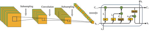
The CNN in the CNN–LSTM model is used to reduce dimensionality and extract high-order features from the input x_t and the output h_t−1 (Bai et al. 2018). Dilated convolutions are introduced in the structure of the CNN to expand the receptive field to the same length of time window through downsampling and aggregate the historical information of different time blocks by increasing the dilation rate of each layer. The look-back window with an interval of 1 is changed to an interval of d_l, which is the dilation rate of the lth layer. In the first hidden layer, the first convolution kernel is placed on the three elements at t, t − 1, and t − 2, the second convolution kernel is placed on the three elements at t, t − 3, and t − 6, and the third convolution kernel is placed on the three elements at t, t − 8, and t − 16, and so on. The dilated convolution formula is as follows: (3) $$\left(W\otimes h\right)\left(l,t,d_l\right)={\displaystyle \sum _{\tau =0}^{\lfloor k/d_l\rfloor }W\left(l,\tau \right)h_{t-d_l\tau }^l}$$(3) where h is the internal state of the lth hidden layer at time t, ⊗ is the convolution operator, W(l, τ) is the weight vector of the l convolution layer in the τth step, τ∈[1, 2, …, τ_max], ⌊ ⌋ is the forward rounding operation, and d_l is the dilation rate of the lth layer.

LSTM is used to select the retained and forgotten data and record the state of a hidden layer. The cell gates in the LSTM network include a forgetting gate, an input gate, and an output gate. The forgetting gate (degree of forgetting) determines the invalid information forgotten by a forgetting unit. The sigmoid activation function is used to output the forgetting gate according to the inputs x_t and h_t−1 in unit C_t−1: (4) $$f_t=\left(W_f\left[h_{t-1},x_t\right]+b_f\right)$$(4) where f_t is the output of a forgetting gate with the range of [0, 1], where 1 and 0 represent retention and forgetting, respectively, and W_f and b_f are the weight matrix and bias term of the forgetting gate, respectively.

The input gate determines the information to be discarded by using the sigmoid activation function to update the output of the input gate and the tanh function to process a cell state: (5) $$i_t=\sigma \left(W_i\left[h_{t-1},x_t\right]+b_i\right)$$(5) where i_t is the output of an input gate, W_i and b_i are the weight matrix and bias term of the input gate, respectively, and σ is the sigmoid activation function.

Similar to the input gate, the output gate uses the sigmoid layer to update information and the tanh layer to process a cell state: (6) $$o_t=\sigma \left(W_o\left[h_{t-1},x_t\right]+b_o\right)$$(6) where o_t is the output gate with the range of [−1, 1], W_o and b_o are the weight matrix and bias term of the output gate, and σ is the sigmoid activation function.

The temperature time-series data {x₁, x₂,…, x_t-1, x_t} are input into the CNN–LSTM model to predict another time series {x₂, x₃,…, x_t, x_t+1}. The temperature x_t+1 at the next time t + 1 can be expressed as (7) $$x_{t+1}=w_t{h}_t+b$$(7) (8) $$h_t=o_t\tanh \left(C_t\right)$$(8) where w_t is the weight connecting the LSTM layer and the output layer, b is the offset of the output layer, h_t is the output value of a neuron, o_t is the output of the input gate, and C_t is the cell state.

The input of the CNN–LSTM is a three-dimensional tensor (batch size, input length, and input channels), where the number of input channels is equal to six key meteorological elements: the daily average, minimum, and maximum temperatures, air pressure, dew point, and wind speed. The output of the CNN–LSTM is also a three-dimensional tensor (batch size, input length, output channels), where the output channels = 1, that is, air temperature.

A subsequence, which is a series of continuous meteorological elements with the input length equal to the convolution kernel size, is input to the CNN–LSTM, and performs a dot product operation with the kernel vector of the learning weights. Stride of the learning is equal to one, which means a convolution kernel window will be moved right to the next position of an element. Each output of a convolution layer is obtained using the same weight vector of convolution kernel. Additional zero values are added to the beginning or end of the input tensor to ensure that the output sequence has the same length as the input sequence. The number of convolution kernel weights is equal to kernel size × input channels × output channels. The number of elements in the intermediate vectors obtained after a convolution operation is equal to the number of input channels. All intermediate vectors are added to obtain the output vector. The above process is repeated for each input channel except for different convolution kernels are used each time.

2.4. Sensitivity analysis of the CNN–LSTM parameters

The Adam algorithm is used to update parameters such as the weight matrix and bias term because it can process sparse gradient and non-stationary targets with small memory requirements. Adam adjusts the learning rate of CNN–LSTM according to the first- and second-order moment estimations of gradient.

The values of parameters such as the number of hidden layers, the number of nodes in each layer, batch size, iteration times, and window length (data sampling interval) have a great impact on the training accuracy of the CNN–LSTM model. Therefore, the value of one parameter was adjusted constantly while the values of the others were left unchanged, and the optimal value of each parameter was determined when the loss function was lowest and the fitting accuracy was best in the training process.

2.5. Evaluation of CNN–LSTM performance

The mean absolute error (MAE), mean absolute percentage error (MAPE), root mean square error (RMSE), and percentage bias (PBIAS) are used to evaluate the performance of the CNN–LSTM model according to the predicted and measured temperatures: (9) $$MAE=\frac{1}{n}{\displaystyle \sum _{i=1}^n|}{P}_i-M_i|$$(9) (10) $$MAPE=\frac{1}{n}{\displaystyle \sum _{i=1}^n|\frac{P_i-M_i}{M_i}}|$$(10) (11) $$RMSE=\sqrt{\frac{1}{n}{\displaystyle \sum _{i=1}^n{\left(M_i-P_i\right)}^2}}$$(11) (12) $$PBIAS=100{\displaystyle \sum _i^n\left(M_i-P_i\right)}/{\displaystyle \sum _i^n\left(M_i\right)}$$(12) where n is the number of samples, and M_i and P_i are the measured and predicted temperatures, respectively, i = 1, 2, …, n.

The closer MAE is to zero, the better the prediction of the model. MAPE and RMSE represent the deviation of the predicted temperature from the measured one. PBIAS represents the average trend between the measured and the predicted temperatures. The smaller the value of PBIAS, the better the prediction performance. A positive PBIAS indicates that the predicted temperature is smaller than the measured one. In contrast, a negative PBIAS indicates that the predicted temperature is larger than the measured one.

Linear regressions between the measured and predicted hourly air temperatures obtained by the CNN, LSTM, and CNN–LSTM models are also used to verify the performance of the CNN–LSTM model. Regression analysis can be used to evaluate prediction accuracy of hourly temperature according to goodness of fit R² between the measured and predicted temperatures, which is the ratio of the explained variance to the total variance of the output (Mba et al. 2016). R² ∈ [0, 1] reflects the degree of agreement between the test data and the fitting function. The closer R² is to one, the better the regression fitting is.

2.6. Prediction process of hourly air temperature

Hourly air temperature is predicted using the CNN–LSTM model as shown in Figure 2.

Figure 2. Flowchart of hourly air temperature prediction using a CNN–LSTM.

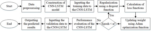
The prediction process of the CNN–LSTM model is as follows:

• Step 1. Initialize the network weight w and the offset vector b, and set the window length L and the maximum number of iterations T.

• Step 2. Standardize the values of the meteorological elements as x′ = {x₁′, x₂′, x₃′,…, x_n′} with the interval of [0, 1].

• Step 3. Divide the data set x′ into the training set x_ts′ = {x₁′, x₂′, x₃′,…, x_b′} and the validation set x_vs′ = {x_b+1′, x_b+2′, x_b+3′,…, x_n′}.

• Step 4. Obtain the predicted value x_t according to the training set x_ts′. Construct a new training set by combining x_ts′ with the L − 1 elements behind x_ts′, and input it to the CNN–LSTM network to obtain the predicted value x_t+1. Finally, a prediction set {x_t, x_t+1, …, x_n} is obtained.

• Step 5. Normalize the data set {x_t, x_t+1, …, x_n} inversely to obtain the predicted hourly temperature set {y_t, y_t+1, …, y_n}.

3. Results

The CNN–LSTM model was established in the Tensorflow framework and Python 3.6. The training set included the meteorological elements of the 204 months from January 2000 to December 2016 in Yinchuan. The validation set included the meteorological elements of the 46 months from January 2017 to October 2020.

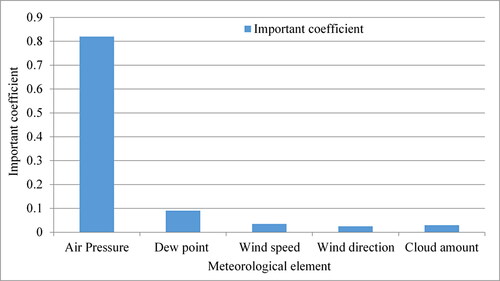
3.1. Selection of meteorological elements

The importance coefficient of each meteorological element was calculated using random-forest method as shown in Figure 3. A meteorological element is highly correlated with air temperature if the OOB error increases significantly after randomly changing the value of the meteorological element. The meteorological elements were sorted in descending order according to their importance. With an importance coefficient of 0.82, air pressure has the greatest impact on hourly air temperature, followed by dew point and wind speed. Therefore, the daily average, minimum, and maximum temperatures, air pressure, dew point, and wind speed were selected as the input variables of the CNN–LSTM model.

Figure 3. Importance coefficients of meteorological elements obtained by random forest.

3.2. Temperatures predicted from CNN–LSTM

The hourly air temperatures measured in Yinchuan from 1 January 2000 to 31 October 2020 were obtained statistically for comparison with the predicted ones as shown in Figure 4(a). The average, maximum, and minimum temperatures in Yinchuan were 10.48, 38.5, and −23.1 °C, respectively.

Figure 4. Comparison of the measured (a) and predicted temperatures (b) from 1 January 2000 to 31 October 2020 and from 1 October 2016 to 10 October 2016 (c) detailed from (b) with a black ellipse and curves of loss function in training and validation stages (d) obtained by CNN–LSTM.

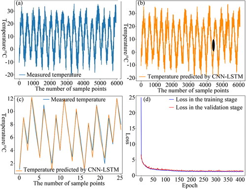
The hourly air temperature in the same period was predicted using the CNN–LSTM model as shown in Figure 4(b). Comparing Figure 4(b) and (a), the CNN–LSTM model has a good fitting effect for long time series of temperature data, especially regarding extreme temperatures.

To verify the generalization ability of the CNN–LSTM model, a short-term sub-dataset of hourly air temperature from 1 October 2016 to 10 October 2016 was selected to compare the predicted and measured temperatures (Figure 4(c)). Most of the predicted temperature curve overlaps with the measured one in the next 10 days. The peaks and troughs of the predicted and measured temperature curves in one day fit very well, with no displacement forward or backward. However, a few peaks and troughs obtained by the CNN–LSTM model are not overlapped by those from the measured temperature. The maximum difference between the predicted and measured temperatures is 1.5 °C, due possibly to data quality and the parameter settings of the model.

Figure 4(d) shows the curves of the loss function in the training and validation stages obtained by the CNN–LSTM model for 400 iterations. The loss curves tend to vary gently as the iterations proceed, and the loss function converges after approximately 100 iterations. The MAE generated by the CNN–LSTM model converges to 0.82 in the training stage and 1.02 in the testing stage (Table 2), which is a very small error between the predicted and measured temperatures. The loss curves from the training and validation sets basically overlap, indicating that the CNN–LSTM model has good generalization ability.

Table 2. Comparison of MAEs, MAPEs, RMSEs, and PBIASs obtained by the CNN, LSTM, and CNN–LSTM models.

Model	In the training stage			In the testing stage
	CNN	LSTM	CNN–LSTM	CNN	LSTM	CNN–LSTM
MAE	1.13	1.08	0.82	1.38	1.29	1.02
MAPE	1.14	0.98	0.63	1.27	1.09	0.8
RMSE	2.96	2.58	2.05	3.14	2.72	1.97
PBIAS/%	15.75	11.39	2.18	16.84	13.21	−0.08

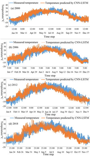
To further verify the generalization ability of the CNN–LSTM model, four sub-datasets of hourly air temperature with one-year interval in 2000, 2006, 2012, and 2018 were selected, respectively, from the dataset of temperature time series. Figure 5 shows the comparison of the measured and predicted hourly temperatures in 2000, 2006, 2012, and 2018 obtained by the CNN–LSTM model. The values of the parameters, such as the number of hidden layers, the number of nodes in each layer, batch size, and iteration times, of the CNN–LSTM model for one-year prediction were set as same as those for short-term prediction. The curves of the predicted hourly air temperatures for one year in advance have strong similarities to those of the measured ones. The predicted and measured hourly temperatures are in a good agreement, which prove the reliability of the CNN–LSTM model for the prediction. However, the deviations between the predicted and measured hourly temperatures with one-year interval are higher than those with 11-day interval (Figure 4(c)).

Figure 5. Comparison of the measured and predicted hourly temperatures obtained by CNN–LSTM with one-year interval in 2000 (a), 2006 (b), and 2012 (c) based on a training set, and 2018 (d) based on a testing set.

3.3. Performance validation of CNN–LSTM based on MAE and MAPE

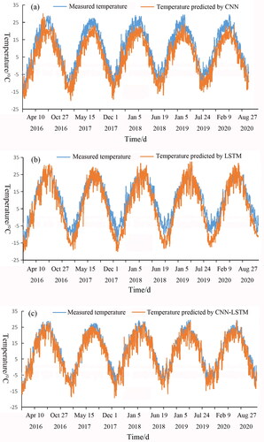
Separate LSTM and CNN models were constructed to validate the performance of the CNN–LSTM model in temperature prediction. Figure 6 shows the measured and predicted temperatures obtained by CNN, LSTM, three models (CNN, LSTM, and CNN–LSTM), and MAPEs obtained by CNN, LSTM, and CNN–LSTM between 1 October 2016 and 10 October 2016, respectively.

Figure 6. Comparison of measured and predicted temperatures obtained by CNN (a), LSTM (b), three models (CNN, LSTM, and CNN–LSTM) (c), MAPEs obtained by CNN, LSTM, and CNN–LSTM (d) between 1 October 2016 and 10 October 2016 detailed from Figure 4(b) with a black ellipse, and the predicted temperatures between 1 January 2016 and 31 January 2016 obtained by three models (e) based on a testing set.

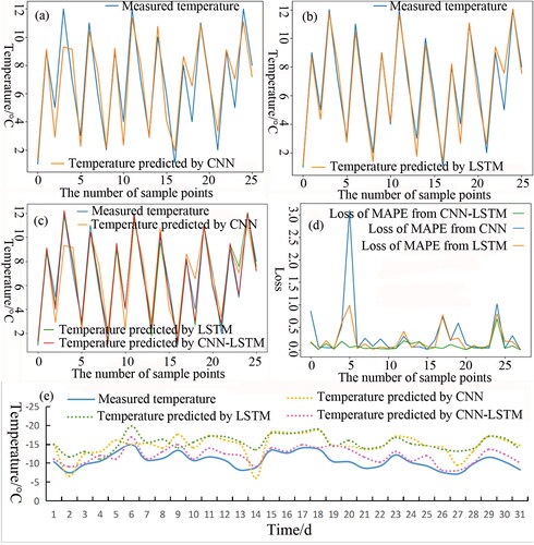
The deviation between the measured temperatures and those predicted by the CNN model is relatively large (Figure 6(a)). The fitting degree of most peaks and troughs in the curve obtained by the CNN model is poor compared with the measured temperature curve. The MAE is large, and its loss function converges to 1.13 in the training stage and 1.38 in the testing stage (Table 2). Therefore, the prediction accuracy of the CNN model is poor.

The fitting degree of the LSTM model for temperature prediction is better than that of the CNN model (Figure 6(b)). However, the peaks and troughs of the predicted temperature curve have large deviations compared with those of the measured temperature curve; some of the predicted temperatures are either larger or smaller than the measured ones. The loss function of the MAE obtained from the LSTM model converges to 1.08 in the training stage and 1.29 in the testing stage, which is smaller than that from the CNN model (Table 2), so the prediction accuracy of the LSTM model is better than that of the CNN model.

Figure 6(c) shows the curves of the measured temperatures and those predicted by the LSTM, CNN, and CNN–LSTM models between 1 October 2016 and 10 October 2016 detailed from Figure 4(b). Of the three models, the peaks, troughs, and temperature curve obtained by the CNN–LSTM model fit best to the measured ones.

Table 2 gives the MAEs, MAPEs, RMSEs, and PBIASs obtained by the CNN, LSTM, and CNN–LSTM models in the training stage and in the testing stage, respectively. The MAEs of the CNN–LSTM model are 27 and 24% in the training stage, and 26 and 21% in the testing stage, lower than those of the CNN and LSTM models, respectively. The MAPEs of the CNN–LSTM model are 45 and 36% in the training stage, and 37 and 27% in the testing stage, lower than those of the CNN and LSTM models, respectively. The RMSEs of the CNN–LSTM model are 31 and 21% in the training stage, and 37 and 28% in the testing stage, lower than those of the CNN and LSTM models, respectively. The PBIASs of the CNN–LSTM model are 86 and 81% in the training stage, and 100.5 and 100.6% in the testing stage, lower than those of the CNN and LSTM models, respectively. The negative PBIAS (−0.08%) obtained from the CNN–LSTM in the testing stage indicates that the predicted temperatures are slightly larger than the measured ones.

Figure 6(d) shows the curves of the MAPEs obtained by the CNN, LSTM, and CNN–LSTM models between 1 October 2016 and 10 October 2016 detailed from Figure 4(b). The separate LSTM and CNN models generate several abnormal MAPEs, but the MAPE curve of the CNN–LSTM model is relatively flat. The temperatures predicted by the CNN–LSTM model fit well with the measured ones, and the MAPE of the CNN–LSTM model is the smallest of the three. Therefore, the CNN–LSTM model has good accuracy in predicting hourly air temperature with long time series and large amounts of data.

The fitting curves of the measured and predicted temperatures from 1 January 2016 to 31 January 2016 obtained from the CNN, LSTM, and CNN–LSTM are shown in Figure 6(e). Three models predict the variation trend of temperature very well. In particular, the temperature predicted by the CNN–LSTM model has the highest fitting degree with the measured temperature. In contrast, the CNN has the largest error between the predicted and measured temperatures. The fitting degree of most peaks and troughs in the curve obtained from the CNN–LSTM model is higher than those obtained from the CNN and LSTM models compared with the measured temperature curve.

3.4. Performance validation of CNN–LSTM based on R²

Figure 7 shows regression lines between the predicted and measured temperatures one-day, one-month, and one-year ahead, respectively, obtained by the CNN–LSTM model. Hourly air temperatures on March 5, March 10, March 15, and March 20 in 2000 were selected as one-day-ahead prediction to obtain regression lines (Figure 7(a–d)). The dotted lines in Figure 7 are the fitted regression lines. The straight lines with a slope of one passing through the origin of coordinate system indicate the simulated temperatures are equal to the measured ones. The values of R² of one-day-ahead prediction of the four days obtained by the CNN–LSTM model are 0.7371, 0.7638, 0.7268, and 0.7544, respectively.

Figure 7. Regression lines between predicted and measured temperatures one-day ahead on March 5 (a), March 10 (b), March 15 (c), and March 20 (d) in 2000, one-month ahead in March (e), June (f), September (g), and December (h) in 2000, and one-year ahead in 2000 (i), 2006 (j), 2008 (k), and 2012 (l) obtained by the CNN–LSTM model based on a training set.

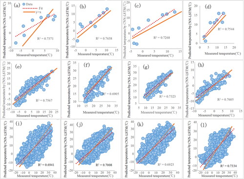
Hourly air temperatures in March, June, September, and December in 2000 were selected as one-month-ahead prediction to obtain regression lines (Figure 7(e–h)). The values of R² of one-month-ahead prediction of the four months obtained by the CNN–LSTM model are 0.7567, 0.6905, 0.7323, and 0.7605, respectively.

Hourly air temperatures in 2000, 2006, 2008, and 2012 were selected as one-year-ahead prediction to obtain regression lines (Figure 7(i–l)). The values of R² for one-year-ahead prediction of hourly air temperatures obtained by CNN–LSTM are 0.6941, 0.7008, 0.6923, and 0.7334, respectively. The CNN–LSTM model had high linear correlation coefficients and gave the best approximation of the measured hourly air temperature for one-day, one-month, and one-year prediction.

To further validate the performance of the CNN–LSTM model for the prediction of hourly air temperature, regression lines between the predicted and measured temperatures one-day, one-month, and one-year ahead are obtained by the CNN and LSTM models (Figure 8). Hourly air temperatures on March 5, March 10, March 15, and March 20 in 2000 were selected as one-day-ahead prediction to obtain regression lines (Figure 8(a–d, m–p)). The values of R² of one-day-ahead prediction of the four days obtained by the CNN model are 0.513, 0.4699, 0.5627, and 0.5126, respectively, which are less than those one-day ahead obtained by the CNN–LSTM model (Table 3). The values of R² of one-day-ahead prediction of the four days obtained by the LSTM model are 0.5027, 0.66, 0.6043, and 0.6321, respectively, which are less than those one-day ahead obtained by the CNN–LSTM model.

Figure 8. Regression lines between predicted and measured temperatures one-day ahead on March 5 (a), March 10 (b), March 15 (c), and March 20 (d) in 2000, one-month ahead in March (e), June (f), September (g), and December (h) in 2000, and one-year ahead in 2000 (i), 2006 (j), 2008 (k), and 2012 (l) obtained by the CNN model, and one-day ahead on March 5 (m), March 10 (n), March 15 (o), and March 20 (p) in 2000, one-month ahead in March (q), June (r), September (s), and December (t) in 2000, and one-year ahead in 2000 (u), 2006 (v), 2008 (w), and 2012 (x) obtained by the LSTM model based on a training set.

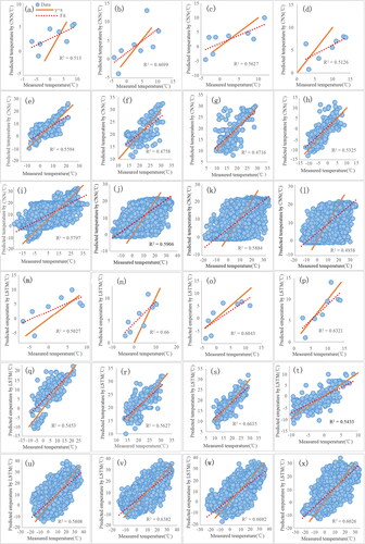
Table 3. Comparison of the values of R² for one-day, one-month, and one-year ahead prediction of hourly air temperatures obtained by CNN, LSTM, and CNN–LSTM.

Time ID	R^2 obtained by CNN–LSTM			R^2 obtained by CNN			R^2 obtained by LSTM
	One day	One month	One year	One day	One month	One year	One day	One month	One year
1	0.7371	0.7567	0.6941	0.513	0.5594	0.5797	0.5027	0.5453	0.5808
2	0.7638	0.6905	0.7008	0.4699	0.4758	0.5906	0.66	0.5627	0.6328
3	0.7268	0.7323	0.6923	0.5627	0.4716	0.5884	0.6043	0.6635	0.6082
4	0.7544	0.7605	0.7334	0.5126	0.5325	0.4938	0.6321	0.5433	0.6026
Average	0.7455	0.735	0.705	0.5146	0.5098	0.5631	0.5998	0.5787	0.6061
Re-average	0.7258			0.5291			0.5949

Hourly air temperatures in March, June, September, and December in 2000 were selected as one-month-ahead prediction to obtain regression lines (Figure 8(e–h, q–t)). The values of R² of one-month-ahead prediction of the four months obtained by the CNN model are 0.5594, 0.4758, 0.4716, and 0.5325, respectively, which are less than those one-month ahead obtained by the CNN–LSTM model. The values of R² of one-month-ahead prediction of the four months obtained by the LSTM model are 0.5453, 0.5627, 0.6635, and 0.5433, respectively, which are less than those one-month ahead obtained by the CNN–LSTM model.

Hourly air temperatures in 2000, 2006, 2008, and 2012 were selected as one-year-ahead prediction to obtain regression lines (Figure 8(i–l, u–x)). The values of R² for one-year-ahead prediction of hourly air temperatures obtained by CNN are 0.5797, 0.5906, 0.5884, and 0.4938, respectively, which are less than those one-year ahead obtained by the CNN–LSTM model. The values of R² for one-year-ahead prediction of hourly air temperatures obtained by LSTM are 0.5808, 0.6328, 0.6082, and 0.6026, respectively, which are less than those one-year ahead obtained by the CNN–LSTM model.

Prediction period, such as the intervals of one day, one month, and one year, has little effect on the accuracy of prediction for hourly air temperature. For example, the average values of R² of one-day, one-month, and one-year predictions obtained by the CNN–LSTM model are 0.7455, 0.735, and 0.705, respectively, with a very small rate of change. However, the CNN–LSTM model can obtain the largest average value of R² (0.7258), which means that predicted hourly air temperatures can adjust to the measured ones better than those obtained by the CNN (R² = 0.5291) and LSTM (R² = 0.5949) models. The sequence of model accuracy from best to worst for predicting hourly air temperature is CNN–LSTM > LSTM > CNN.

3.5. Performance validation of CNN–LSTM based on the testing set

Figure 9 shows the curves of the measured and predicted temperatures obtained from the CNN (Figure 9(a)), LSTM (Figure 9(b)), and CNN–LSTM (Figure 9(c)) based on the testing set of air temperatures from 1 January 2016 to 31 December 2020. The change of temperature predicted from the CNN was basically consistent with that of the measured temperatures (Figure 9(a)). There was no lagged displacement deviation between the measured and the predicted temperatures. However, there were large errors between the measured annual maximum temperatures and the predicted ones and between the annual minimum temperatures and the predicted ones. The predicted temperatures, especially the annual maximum and minimum temperatures, were smaller than the measured temperatures.

Figure 9. Comparison of measured and predicted temperatures from 2016 to 2020 obtained by CNN (a), LSTM (b), and CNN–LSTM (c) based on a testing set.

The LSTM model generated a better fitting effect on the change of temperatures than the CNN model (Figure 9(b)). Like the CNN model, lagged displacement deviation between the measured and predicted temperatures obtained from the LSTM is not found. However, there were large errors between the predicted and measured annual maximum temperatures and between the predicted and measured annual minimum temperatures. Most predicted temperatures were lower than the measured temperatures. The predicted annual temperature range was larger than the measured one. The predicted annual maximum temperatures were higher than the measured ones, and the predicted annual minimum temperatures were lower than the measured ones.

The CNN–LSTM obtained the best prediction accuracy during the testing stage of the deep leaning compared with the CNN and LSTM, especially for the high and low temperatures in a long time-series temperatures (Figure 9(c)). The temperatures predicted by the CNN–LSTM model coincided with the measured temperatures except for a few predicted abnormal annual minimum temperatures. Like the CNN and LSTM, there is no lag displacement deviation between the predicted and the measured temperatures.

3.6. Comparison of box plots based on the training and testing sets

Box plot is used to show the distribution of the temperature time-series data because it is not need to assume that the data obey a specific distribution form in advance, and does not have any restrictive requirements on the data. The temperatures collected from 1 January 2000 to 31 December 2015 are used as the observation data. The temperatures collected from 1 January 2016 to 31 December 2020 are used as the testing data. The CNN–LSTM model is used to train the observation data and validate its performance according to the testing data. Box plots are constructed with the four groups of data (measured temperatures for the training and testing of the CNN–LSTM and temperatures predicted from the training and testing of the CNN–LSTM; Figure 10).

Figure 10. Analysis of box plots based on the training and testing sets.

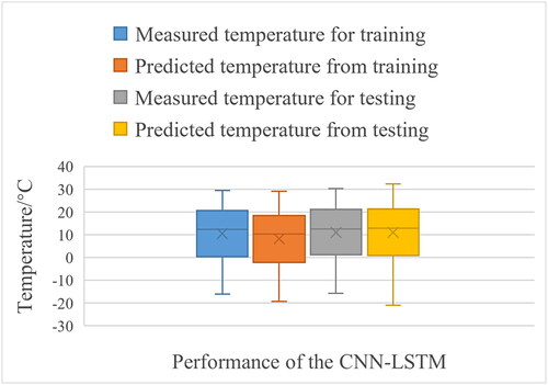
The box plots show the distribution characteristics of the maximum, minimum, median, and upper and lower quartiles of the measured temperatures in the training stage and the predicted temperatures in the testing stages. The quartiles and interquartile distances in the four box-plots show that there are no outliers in the four groups of data. The lengths and interquartile distances of the four box-plots are the same, indicating that the concentration and dispersion of the four groups of data are the same. The medians of the four groups of data are all located at the upper parts of the box plots, indicating that the four groups of data are left-skewed distribution.

The maximum, minimum, median, and average of the observed temperatures, which are used to test the performance of the CNN–LSTM (the third box plot in Figure 10), are slightly higher than those used to train the CNN–LSTM (the first box plot in Figure 10). The result shows the increasing in temperature year by year. The maximum, minimum, upper quartile, lower quartile, median, and average of the temperatures predicted from the training of the CNN–LSTM (the second box plot in Figure 10) are smaller than those of the observed temperatures used to train the CNN–LSTM (the first box plot in Figure 10). The upper quartile, lower quartile, median, and average of the temperatures predicted from the testing of the CNN–LSTM (the fourth box plot in Figure 10) are equal to those of the observed temperatures used to test the performance of the CNN–LSTM (the third box plot in Figure 10), while the maximum value is larger, and the minimum value is smaller, than those of the observed temperatures used for testing. The maximum, minimum, upper quartile, lower quartile, median, and average of the temperatures predicted from the testing (the fourth box plot in Figure 10) are larger than those predicted from the training (the second box plot in Figure 10). Although the characteristics of the box plots for the temperatures predicted from the training and testing are different from those for the observed temperatures used for training and testing, the difference is very small. Therefore, the CNN–LSTM can predict the temperature time-series data with high accuracies in the training and testing stages.

4. Discussion

The accurate prediction of hourly air temperature promotes plan establishment for business development, agricultural and industrial activities, and energy policy. Deep learning method can extract different characteristics of hourly temperature in a dataset by learning the long-term dependence between parameters to solve the dynamic instability of time series. The CNN–LSTM model has good accuracy in predicting hourly air temperature with long time series and large amounts of data. CNN in the CNN–LSTM model can process high-dimensional data, share convolution kernel, eliminate data noise, retain stable gradient, and extract high-order features automatically. While LSTM in the CNN–LSTM model can remember the time-series characteristics of air temperature with long-term dependence, and reduce the risk of over fitting (Hochreiter and Schmidhuber 1997).

The choices regarding iterations, batch size, window length, learning rate, and optimizer type have a great impact on the accuracy of air temperature (Hanoon et al. 2021). A deep-learning model might not converge with too small iterations but might over-fit with too large iterations. With too small batch size, the loss function might continue to decease, resulting in the model failing to converge; however, with too large batch size, the training rate might decrease, the training time might increase, and the computer equipment configuration might become higher than before. A large window length might cause some feature information to be lost, whereas a small window length might lead to data redundancy and reduce training speed. A small learning rate might cause slow decline of loss function, whereas a large learning rate might cause gradient explosion. Also, a good optimizer helps to improve the learning rate and the updating of weights to prevent over-fitting.

The sizes of the training and testing datasets influence on the performance of the CNN–LSTM model to predict the accuracy of hourly air temperature. The minimum size of training dataset should be determined after calculating all the variants of temperature time series. The minimum size of testing set is determined according to the minimum size of training dataset. The prediction accuracy of the training dataset with the minimum size should be compared with those with other sizes to analyze the impact of dataset size on the performance of the CNN–LSTM model.

Sequential sensitivity of the CNN–LSTM model should be tested using samples selected sequentially from a time series of dataset as input according to MAEs, MAPEs, RMSEs, and PBIASs of the model. The CNN–LSTM model can predict hourly temperatures with good accuracy within 48 h because the temperature time series are strongly correlated with different hourly interval times. However, the accuracy will gradually decline from medium-term, such as monthly interval time, to long-term, such as yearly interval time, prediction of hourly temperature time series. Short-, medium-, and long-terms samples should be selected, respectively, to test the sensitivity of the CNN–LSTM model.

Temperature time series data with hourly, daily, monthly, and annual intervals between different meteorological stations should be collected as the input of the CNN–LSTM model to verify the generalization ability of the model. Meteorological elements, such as air pressure, relative humidity, hourly precipitation, maximum wind speed, minimum visibility, solar radiation, water vapor pressure, and wind direction, might affect the prediction accuracy of hourly air temperatures. Therefore, more elements should be collected as many as possible to improve the prediction accuracy of the CNN–LSTM model.

The meteorological elements in Yinchuan meteorological station were collected in this study. However, those in adjacent meteorological stations of Yinchuan are not collected. Spatial locations of meteorological stations might have a certain impact on prediction results (Nury et al. 2017). In the future, the longitude and latitude coordinates and other spatial information, such as altitude, of adjacent meteorological stations should be collected.

Selecting the best input variables, including meteorological and geographical variables, for a particular deep-learning method is difficult because of the complexity and nonlinearity of temperature time series. The effect of relevant meteorological, such as maximum, minimum, and mean rainfall, temperature, and relative humidity, and geographical variables, such as longitude, latitude, and elevation, should be analyzed to improve the prediction accuracy of hourly air temperature (Murat et al. 2016). The useful input variables to predict hourly air temperature can be selected using feature selection methods, such as random forest, recursive feature elimination, and correlation coefficient.

5. Conclusion

Hourly air temperature prediction was performed by combining LSTM and a CNN (CNN–LSTM) to extract dynamic meteorological features according to network memorability. Future hourly temperatures were predicted using meteorological data obtained from January 2000 to December 2020 in Yinchuan, China. The experimental results show that of the CNN–LSTM model and separate CNN and LSTM models, the CNN–LSTM model has the best accuracy with an MAE, MAPE, RMSE, and PBIAS of 0.82, 0.63, 2.05, and 2.18 in the training stage and an MAE, MAPE, RMSE, and PBIAS of 1.02, 0.8, 1.97, and −0.08 in the testing stage. The temperature curve and its peaks and troughs obtained by the CNN–LSTM model fitted best to the measured ones compared with those given by the LSTM and CNN models. The average goodness of fits of regression lines one-day, one-month, and one-year ahead obtained by the CNN–LSTM, CNN, and LSTM model are 0.7258, 0.5291, and 0.5949, respectively. From best to worst, the sequence of model accuracy for predicting hourly air temperature is CNN–LSTM > LSTM > CNN. Therefore, the CNN–LSTM model can be used to improve the generalization and fault toleration for high-accuracy hourly temperature prediction with large amounts of meteorological data.

A graph network should be constructed using multiple meteorological stations. A graph convolutional network (GCN) should be constructed to extract spatial characteristics of temperature data (Zhu et al. 2022). A GRU should be constructed to extract the temporal characteristics of temperature data. The matrix multiplication of GRU can be replaced by a graph convolution operation to capture the spatiotemporal relationship of temperature data. A connection method of multi-order nearest neighbors should be used in GCN to reduce MAEs and MAPEs of a prediction model (Chhetri et al. 2020).

Disclosure Statement

No potential conflict of interest was reported by the authors.

Data availability statement

Dataset(s) derived from public resources and made available with the article. The datasets analysed during the current study are available in the [the National Oceanic and Atmospheric Administration (NOAA) of the United States] repository. These datasets were derived from the following public domain resources: [https://psl.noaa.gov/data/gridded/tables/temperature.html; ftp://ftp.ncdc.noaa.gov/pub/data/noaa/isd-lite/]

Correction statement

This article was originally published with errors, which have now been corrected in the online version. Please see Correction (http://dx.doi.org/10.1080/19475705.2022.2113684)

Additional information

Funding

This work was supported by the Natural Science Foundation of Ningxia Province in China [grant number 2022AAC03055].

References

- Abdollahi A, Pradhan B, Alamri A. 2020. An ensemble architecture of deep convolutional Segnet and Unet networks for building semantic segmentation from high-resolution aerial images. Geocarto Int. 3:1–16.
- Al-Najjar H, Kalantar B, Pradhan B, Saeidi V, Abdul HA, Ueda N, Mansor S. 2019. Land cover classification from fused DSM and UAV images using convolutional neural networks. Remote Sens. 11(12):1461.
- Asha J, Santhosh KS, Rishidas S. 2021. Forecasting performance comparison of daily maximum temperature using ARMA based methods. J Phys- Conf Ser. 1921(1):012041.
- Astsatryan H, Grigoryan H, Poghosyan A, Abrahamyan R, Asmaryan S, Muradyan V, Tepanosyan G, Guigoz Y, Giuliani G. 2021. Air temperature forecasting using artificial neural network for Ararat valley. Earth Sci Inform. 14(2):711–722.
- Bahi M, Batouche M. 2021. Convolutional neural network with stacked autoencoders for predicting drug-target interaction and binding affinity. IJDMMM. 13(1/2):81–−113.
- Bai S, Kolter JZ, Koltun V. 2018. An empirical evaluation of generic convolutional and recurrent networks for sequence modeling. arXiv:1803.01271.
- Bai P, Liu XM, Xie JX. 2021. Simulating runoff under changing climatic conditions: A comparison of the long short-term memory network with two conceptual hydrologic models. J Hydrol. 592(1):125779.
- Bayatvarkeshi M, Bhagat SK, Mohammadi K, Kisi O, Farahani M, Hasani A, Deo R, Yaseen ZM.,. 2021. Modeling soil temperature using air temperature features in diverse climatic conditions with complementary machine learning models. Comput Electron Agr. 185:106158.
- Bonjakovi B. 2012. Geopolitics of climate change: a review. Therm Sci. 16(3):629–−654.
- Byeongseong C, Mario B, Elie BZ, Matteo P. 2021. Short-term probabilistic forecasting of meso-scale near-surface urban temperature fields. Environ Modell Softw. 145(11):105189.
- Carrión D, Arfer KB, Rush J, Dorman M, Rowland ST, Kioumourtzoglou MA, Kloog I, Just AC. 2021. A 1-km hourly air-temperature model for 13 northeastern U.S. states using remotely sensed and ground-based measurements. Environ Res. 200:111477.
- Chevalier RF, Hoogenboom G, , Mcclendon RW, , Paz JA. 2011. Support vector regression with reduced training sets for air temperature prediction: a comparison with artificial neural networks. Neural Comput Appl. 20(1):151–−159.
- Chhetri M, Kumar S, Roy PP, Kim BG. 2020. Deep BLSTM-GRU model for monthly rainfall prediction: a case study of Simtokha, Bhutan. Remote Sens-Basel. 12(19):3174–3187.
- Ferreira PM, Faria EA, Ruano AE. 2002. Neural network models in greenhouse air temperature prediction. Neurocomputing. 43(1-4):51–75.
- Gos M, Krzyszczak J, Baranowski P, Murat M, Malinowska I. 2020. Combined TBATS and SVM model of minimum and maximum air temperatures applied to wheat yield prediction at different locations in Europe. Agr Forest Meteorol. 281:107827.
- Hanoon MS, Ahmed AN, Zaini N, Razzaq A, Kumar P, Sherif M, Sefelnasr A, El-Shafie A. 2021. Developing machine learning algorithms for meteorological temperature and humidity forecasting at Terengganu state in Malaysia. Sci Rep. 11(1):18935–18935.
- Hochreiter S, Schmidhuber J. 1997. Long short-term memory. Neural Comput. 9(8):1735–−1780.
- Immerzeel WW, Beek LPH, Bierkens MFP. 2010. Climate change will affect the Asian water towers. Science. 328(5984):1382–−1385.
- Jiang HW, Qin FW, Cao J, Peng Y, Shao YL. 2021. Recurrent neural network from adder’s perspective: Carry-look ahead RNN. Neural Netw. 144:297–−306.
- Johnson ZC, Johnson BG, Briggs MA, Devine WD, Snyder CD, Hitt NP, Hare DK, Minkova TV. 2020. Paired air-water annual temperature patterns reveal hydrogeological controls on stream thermal regimes at watershed to continental scales. J Hydrol. 587:124929.
- Kattenborn T, Leitloff J, Schiefer F, Hinz S. 2021. Review on convolutional neural networks (CNN) in vegetation remote sensing. ISPRS J Photogramm. 173:24–−49.
- Li ZL, Tang BH, Wu H, Ren HZ, Yan GJ, Wan ZM, Trigo IF, Sobrino JA. 2013. Satellite-derived land surface temperature: current status and perspectives. Remote Sens Environ. 131:14–37.
- Lin ML, Tsai CW, Chen CK. 2021. Daily maximum temperature forecasting in changing climate using a hybrid of multi-dimensional complementary ensemble empirical mode decomposition and radial basis function neural network. J Hydrol-Reg Stud. 38(12):100923.
- Liu Z, Zhan W, Lai J, Hong F, Quan J, Bechtel B, Huang F, Zou Z. 2019. Balancing prediction accuracy and generalization ability: A hybrid framework for modelling the annual dynamics of satellite-derived land surface temperatures. ISPRS J Photogramm. 151:189–206.
- Livera AMD, Hyndman RJ, Snyder RD. 2011. Forecasting time series with complex seasonal patterns using exponential smoothing. J Am Stat Assoc. 106(496):1513–−1527.
- Mba L, Meukam P, Kemajou A. 2016. Application of artificial neural network for predicting hourly indoorair temperature and relative humidity in modern building in humid region. Energy Build. 121:32–42.
- Moazenzadeh R, Mohammadi B, Duan Z, Delghandi M. 2022. Improving generalisation capability of artificial intelligence-based solar radiation estimator models using a bio-inspired optimisation algorithm and multi-model approach. Environ Sci Pollut Res Int. 29(19):27719–27737.
- Mohammadi B, Mehdizadeh S, Ahmadi F, Lien NTT, Linh NTT, Pham QB. 2021. Developing hybrid time series and artificial intelligence models for estimating air temperatures. Stoch Environ Res Risk Assess. 35(6):1189–1204.
- Mtibaa F, Nguyen KK, Azam M, Papachristou A, Venne JS, Cheriet M. 2020. LSTM-based indoor air temperature prediction framework for HVAC systems in smart buildings. Neural Comput Appl. 32(23):17569–−17585.
- Murat M, Malinowska I, Gos M, Krzyszczak J. 2018. Forecasting daily meteorological time series using ARIMA and regression models. Int Agrophys. 32(2):253–−264.
- Murat M, Malinowska I, Hoffmann H, Baranowski P. 2016. Statistical modelling of agrometeorological time series by exponential smoothing. Int Agrophys. 30(1):57–−65.
- Murthy KVN, Saravana R, Kumar GK, Kumar KV. 2021. Modelling and forecasting for monthly surface air temperature patterns in India, 1951–2016: Structural time series approach. J Earth Syst Sci. 130(1):21.
- Nury AH, Hasan K, Alam MJB. 2017. Comparative study of wavelet-ARIMA and wavelet-ANN models for temperature time series data in northeastern Bangladesh. J King Saud Univ Sci. 29(1):47–−61.
- Ortiz-Garcia EG, Salcedo-Sanz S, Casanova-Mateo C, Paniagua-Tineo A, Portilla-Figueras JA. 2012. Accurate local very short-term temperature prediction based on synoptic situation support vector regression banks. Atmos Res. 107:1–8.
- Patel J, Shah S, Thakkar P, Kotecha K. 2015. Predicting stock and stock price index movement using trend deterministic data preparation and machine learning techniques. Expert Syst Appl. 42(1):259–−268.
- Pradhan B, Al-Najjar HAH, Maher I, Tsang I, Alamri AM. 2020. Unseen land cover classification from high-resolution Orthophotos using integration of Zero-Shot learning and convolutional neural networks. Remote Sens. 12(10):1676.
- Prior MJ, Perry MC. 2014. Analyses of trends in air temperature in the United Kingdom using gridded data series from 1910 to 2011. Int J Climatol. 34(14):3766–−3779.
- Radhika Y, Shashi M. 2009. Atmospheric temperature prediction using support vector machines. Int J Comput Theory Eng. 1(1):55–58.
- Ramesh K, Anitha R. 2014. MARSpline model for lead seven-day maximum and minimum air temperature prediction in Chennai. J Earth Syst Sci. 123(4):665–672.
- Rowland ST, Boehme AK, Rush J, Just AC, Kioumourtzoglou MA. 2020. Can ultra short-term changes in ambient temperature trigger myocardial infarction? Environ Int. 143:105910.
- Şahin M. 2012. Modelling of air temperature using remote sensing and artificial neural network in Turkey. Adv Space Res. 50(7):973–985.
- Sekertekin A, Bilgili M, Arslan N, Yildirim A, Celebi K, Ozbek A. 2021. Short-term air temperature prediction by adaptive neuro-fuzzy inference system (ANFIS) and long short-term memory (LSTM) network. Meteorol Atmos Phys. 133(3):943–959.
- Shi L, Kloog I, Zanobetti A, Liu P, Schwartz JD. 2015. Impacts of temperature and its variability on mortality in New England. Nat Clim Chang. 5:988–991.
- Srivastava T, Vedanshu, Tripathi MM. 2020. Predictive analysis of RNN, GBM and LSTM network for short-term wind power forecasting. J Stat Manag Syst. 23(1):33–−47.
- Sun L, Wang WY, Jia C, Liu XR. 2021. Leaf area index remote sensing based on Deep Belief Network supported by simulation data. Int J Remote Sens. 42(20):7637–−7661.
- Tabrizi SE, Xiao K, Van Griensven Thé J, Saad M, Farghaly H, Yang SX, Gharabaghi B. 2021. Hourly road pavement surface temperature forecasting using deep learning models. J Hydrol. 603:126877.
- Tasadduq I, Rehman S, Bubshait K. 2002. Application of neural networks for the prediction of hourly mean surface temperatures in Saudi Arabia. Renew Energ. 25(4):545–554.
- Tran TTK, Bateni SM, Ki SJ, Vosoughifar H. 2021. A review of neural networks for air temperature forecasting. Water. 13(9):1294–1294.
- Ustaoglu B, Cigizoglu HK, Karaca M. 2008. Forecast of daily mean, maximum and minimum temperature time series by three artificial neural network methods. Met Apps. 15(4):431–−445.
- Xiao C, Chen N, Hu C, Wang K, Gong J, Chen Z. 2019. Short and mid-term sea surface temperature prediction using time-series satellite data and LSTM-Adaboost combination approach. Remote Sens Environ. 233:111358.
- Yang C, Hou JW, Wang YJ. 2021. Extraction of land covers from remote sensing images based on a deep learning model of NDVI-RSU-Net. Arab J Geosci. 14(20):2073.
- Ye L, Yang G, Ranst EV, Tang H. 2013. Time-series modeling and prediction of global monthly absolute temperature for environmental decision making. Adv Atmos Sci. 30(2):382–−396.
- Zhang Z, Dong Y. 2020. Temperature forecasting via convolutional recurrent neural networks based on time-series data. Complexity. 2020:1–8.
- Zhang Y, Yu C, Wang L. 2017. Temperature exposure during pregnancy and birth outcomes: an updated systematic review of epidemiological evidence. Environ Pollut. 225:700–712.
- Zhu K, Zhang S, Li JS, Zhou D, Dai H, Hu ZQ. 2022. Spatiotemporal multi-graph convolutional networks with synthetic data for traffic volume forecasting. Expert Syst Appl. 187:115992.