Reconstruction of liquefaction damage scenario in Northern Bihar during 1934 and 1988 earthquake using geospatial methods

Abstract

Northern Bihar witnessed severe liquefaction events during the 1934 (8.2 Mw) and 1988 (6.9 Mw) earthquakes. This study reconstructed the liquefaction damage scenario due to both earthquakes (1934, 1988). The liquefaction hazard map was prepared using two techniques (1) Rapid Response and Loss Estimation (Model A) and (2) the (Model B) Liquefaction Susceptibility Map (LSM) integrated with the Peak Ground Acceleration (PGA). The LSM was prepared using the multicriteria decision-making technique considering the site-specific thematic layers. The ground motion parameters (PGV and PGA) were retrieved from isoseismal maps prepared for both events. The hazard map prepared using Model B was classified into four classes very low, low, high, and severe, and the results obtained from both models were compared. The area under the curve (AUC) was determined for Model A 0.88 and 0.85 and Model B 0.94 and 0.84 for the 1934 and 1988 earthquakes, respectively. The prepared liquefaction hazard map may help policymakers demarcate the study area according to liquefaction hazard potential and mitigate future hazards.

Keywords:

• PGA
• PGV
• liquefaction
• site-specific

1. Introduction

The Northern Bihar in the eastern Ganga plain witnessed severe destruction due to earthquakes in the last 100 years. The great earthquake of 8.2 Mw (Sapkota et al. 2016) struck Bihar in 1934, causing extensive damage. Houses were slanted and buried in the soil from Bettiah to Purnea; another earthquake of magnitude 6.9 Mw occurred near the Nepal-Bihar border on August 21, 1988, causing damage to houses and structures (Mukarjee and Lavania 1998). The Indo-Gangetic plains are located near the Himalayan fault system, which has the potential to generate large earthquakes. The unconsolidated Holocene sediments of IGP deposited from the Ganga, Yamuna, and other tributary rivers create an ideal environment for liquefaction.

To estimate liquefaction potential, field and laboratory investigations were conducted in selected cities in the Indo-Gangetic plains, including Delhi, Patna, Allahabad, Kanpur and surrounding areas. It was shown that the cities of Patna and Allahabad are more prone to liquefaction than Kanpur (Naik et al. 2022). The Indian capital Delhi has severe-to-moderate liquefaction potential assessed by Rao and Satyam (2007). According to a field test conducted by Sitharam et al. (2013), a major chunk of Lucknow city has been classified as liquefaction vulnerable.

The IGP is made mostly of unconsolidated recent Holocene sediments that are prone to liquefaction following an earthquake. The PGA for IGP varies from 0.1 to 0.4 for a 10% probability of exceedance in 50 years and 0.3–1 for a 2% probability of exceedance in 50 years, according to the PSHA done by Nath and Thingbaijam (2012). Devastating earthquake damage in 1833 Nepal (7.6 Mw), 1934 Nepal-Bihar (8.2 Mw), 1988 Bihar-Nepal (6.9 Mw), 2011 Sikkim (6.9 Mw), and 2015 Nepal established the IGP's previous seismic hazard potential (7.8 Mw). During the 1934 Nepal-Bihar earthquake, the MMI ranged from V to IX, and in 1988, it was IV to IX in the IGP (Nath et al. 2019).

Variations in earthquake intensity are controlled by the geographical location and lithological conditions of the region. In addition to structural damage, landslides were frequent in the mountainous area, and liquefaction was seen in the alluvial plains during earthquakes. Severe liquefaction occurrences have been seen in Northern Bihar as a result of the earthquakes in 1934 and 1988 (Mar 1991; Gupta 1994). Liquefaction occurs when pore water pressure increases during earthquake shaking, and the soil’s stiffness significantly reduces. The increased pore water pressure transforms soil from a solid to a liquid state, which causes the liquefied soil to reach the surface, resulting in soil settlement and tilting of structures (Dixit et al. 2012).

Liquefaction is typically seen in saturated, unconsolidated soils (Seed and Idriss 1971; Satyam 2012; Nath et al. 2018; Putti and Satyam 2018). It is dependent on the properties of the soil, earthquakes intensity and environmental conditions (Satyam 2012). Considerable risk of liquefaction exists for sediments deposited in river environments and in areas with shallow groundwater tables (Youd and Hoose 1977). The leading causes of liquefaction are soil parameters and earthquake characteristics including relative density, grain size distribution, intensity, and ground motion duration (Seed and Idriss 1971; Dixit et al. 2012; Satyam 2012).

In order to assess the liquefaction potential of soils, some studies have utilized field-based procedures as the standard penetration test, cone penetration test, and shear wave test (Seed and Idriss 1971; Iwasaki et al. 1984; Robertson and Wride 1996; Andrus et al. 2000). Further, the simplified procedure proposed by Seed and Idriss (1971) was updated by Youd et al. (2001), and various recommendations were provided to enhance the model’s applicability. While the in-situ approaches for liquefaction hazard assessment are accurate, the processes were expensive, time-consuming, and labor-intensive. Although geospatial models may not be the substitute, the advantages associated with technology should be utilized.

Geospatial approaches were used very infrequently to conduct studies on liquefaction hazard assessment. The benefit of the geospatial technique is that it contributes to the fastest and least expensive regional understanding of the liquefaction event. Using parameters such surface roughness, shear wave from topographic slope, distance to the coast and water body, soil type, and ground motion parameter, a logistic regression approach was developed by Zhu et al. (2017), Bozzoni et al. (2021). Karpouza et al. (2021) evaluated the liquefaction using factors such as the age of the soil, compound topographic index, PGA, distance to streams, and site class. Additionally, lithological and geomorphological parameters were used to determine the likelihood of liquefaction (Ganapathy and Rajawat 2012). Pudi et al. (2019), established an analytical hierarchy process (AHP) based model where site-specific characteristics responsible for liquefaction were taken into account for susceptibility mapping.

The site-specific properties of the area define the possibility for liquefaction, whereas shaking is a triggering force necessary to cause a subsurface layer to liquefy. Several groundmotion parameters are used to quantify earthquake shaking; in this work, PGA was employed; these parameters are the driving force behind liquefaction; the PGA layer was independently integrated with the AHP model’s hazard map. Several historical occurrences and research have demonstrated that the North-Bihar area is subject to liquefaction risks, placing a huge population at danger. Because the study region lacked liquefaction hazard maps, we attempted to reproduce the liquefaction situation for the 1934 and 1988 earthquakes. The challenge here is determining whether the geospatial parameters used correlate with the processes causing liquefaction; the geospatial data used were derived from available research. The goal of the study was to assess the liquefaction damage scenario in prior earthquakes and propose ideas for future disasters.

This study used a rapid response and loss estimation model (Model A) and an AHP model (Model B) to prepare the liquefaction map for the 1934 and 1988 events. Liquefaction maps created using both methodologies were compared and validated; these maps might serve as reference data for future liquefaction hazard evaluations. Groundwater, structure density, soil texture, drainage buffer, deposit age, and geomorphology were the factors employed for the liquefaction map. PGA values generated due to reference earthquakes were not available, so the MMI (modified mercalie intensity) values were converted using the relationship proposed by Anbazhagan et al.,(2016). The hazard maps were validated using reference information from previously published literature and reports.

2. Study area

The Northern Bihar Figure 1 is a part of the eastern Ganga plains was considered for this research work. Dunn et al. (1939) provided thorough documentation of the great Bihar earthquake that occurred on January 15, 1934; the epicentre is indicated as being at 26.58 N and 86.58 E, about 60 km south of the MBT, with a magnitude of Ms 8.4 and a depth of 30 km (Richter 1958). The instrumentally relocated epicentre is located approximately 10 km south of Mt Everest at 27.55°N, 87.09°E (Chen and Molnar 1977), whereas many catalogues incorrectly retain Richter’s early erroneous Bihar epicentre nearly 200 km to the south. Singh and Gupta (1980) determined that this earthquake was caused by a combination of thrust and strike-slip fault mechanisms. Based on geodetic data, (Bilham et al. 1998) proposed that the rupture ended to the north of the Indian border; they ruled out the possibility that the rupture ended to the south, as (Seeber and Armbruster 1981). There is no evidence of faulting in the basement, and several observations suggest that the slumping was only superficial (Dunn et al. 1939; Molnar and Pandey 1989). The rupture zone is most likely beneath eastern Nepal’s Lesser Himalaya. The most severe destruction occurred along a 100-kilometer stretch parallel to the Himalaya, but destruction was not insignificant in the 300-kilometer stretch from Nepal’s eastern border to just west of Kathmandu. As a result, the rupture zone’s length is best described as 200 ± 100 km. The mesoseismal area with intensities ≥ VIII, covered more than 10,000 km² (Ambraseys and Douglas 2004; Sapkota et al. 2013; 2016). Chronicles also report triggered landslides along much of eastern Nepal. Liquefaction and slumping affected a 300-km long region farther south in Bihar.

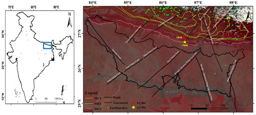
Figure 1. The major thrust faults, lineaments, and faults overlayed on the study area and the Satellite (Landsat OLI) image depicting the Northern Bihar region used for the liquefaction hazard assessment.

On 21 August, 1988 at 04: 55 a.m. an earthquake of magnitude of 6.9 Mw rocked eastern Nepal (Banghar 1991; Baruah et al. 2018). The epicenter of the earthquake was located in Udayapur district to the south of Siwalik hills and depth was 57 km. The seismic source parameters of the 1988 earthquake are well estimated thanks to the advent of the global digital seismic network: the epicentre at 26.728 N and 86.638 E, Mw 6.9, and depth 55–65 km (USGS, ISC and ERI). The GSI (1993) concluded that both of these events are deeper and caused by the East Patna fault, a long transverse fault that runs across the Indo-Gangetic plain and transverse to the Himalayan trend.

(Mukhopadhyay 1984; Kayal 2001) also argued that the central and eastern Himalayas’ transverse faults and subsurface ridges are seismogenic sources in the foothills region, and earthquakes occur primarily through strike-slip mechanisms. These findings indicate that the 1934 Great Bihar earthquake was not caused by a plane of detachment in the Himalayan seismic belt. Further evidence suggests that the source zone of the recent 1988 earthquake is significantly deeper (50 km) in the uppermost mantle of the under-thrusting Indian plate and that the source zone is linked to a transverse fault in the foredeep or foothills.

The sediment thickness in the foredeep basin in front of the Himalayas ranges from a few metres in the South to 1500–2500 m in the North (Valdiya 2016). The study area drained by rivers Gandak, Budhi Gandak, Bagmati, Kamla-Balan, Kosi and Mahananda. As a result of massive sedimentation of rivers and its closeness to the very active tectonic belt Himalaya, the IGP is vulnerable to destruction (Keshri et al. 2020).

Soil liquefaction occurs in cohesionless saturated sediments, and alluvial plains are ideal locations for such deposits; Figure 1 illustrates the research area’s Lithology map. North Bihar has a dense population; given the severity of prior liquefaction events, the region was chosen as the study area for the research.

The Main Central Thrust, Main Boundary Thrust, and the Himalayan Frontal Thrust are all parts of a highly active Himalayan fault system that is situated in the north of the study area (Verma and Bansal 2013; Philip et al. 2014). The Munger-Sehersa ridge and Madhubani Purnia depression are tectonic structures in the study area depicted in Figure 2 that have an influence on the region’s sedimentation and tectonic history (Dasgupta et al. 1987; Valdiya 2016). The study area has two basement faults: the West Patna Fault (WPF) and the East Patna Fault (EPF). The East Patna Fault was linked to the earthquakes of 1934 and 1988 (Verma et al. 2017). The Gandak fault influences the river, and it has also been noted that the river is moving eastward (Mohindra et al. 1992; Anbazhagan et al. 2015).

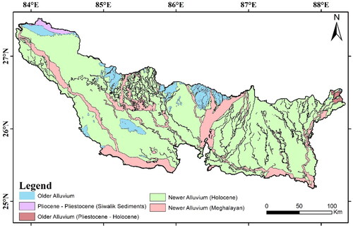
Figure 2. The lithological map of the study area showing different geological units classified in older alluvium from Pliocene to newer alluvium Meghalayan (BHUKOSH, GSI).

The intensity of earthquake-induced damage is categorized using the Modified Mercallie Intensity scale (MMI) (Wood & Neumann, 1931). Roman numerals from I to X (USGS) are used to classify damage based on the severity of the hazard. Northern Bihar is categorized as being in the Vth and IVth zones by India’s BIS, suggesting that there is a high risk of earthquake damage.

3. Methodology and materials used

The rapid response and loss estimation model (Model A) proposed by Zhu et al. (2017) and an AHP model (Model B) were used in this study to produce liquefaction hazard maps for the earthquakes that occurred in 1934 and 1988. The AHP method is widely used and employed for a variety of geological hazard evaluations. This method was used to construct the liquefaction susceptibility map, which was then combined with the PGA to create the final hazard map.

3.1. Liquefaction map using rapid response and loss estimation model (model A)

The risk of soil liquefaction is influenced by seismic stress, soil saturation, and soil density, several explanatory variables that strongly resemble these parameters were studied in (Zhu et al. 2017). The parameters used for model preparation included PGV for earthquake loading, shear wave for soil density and precipitation, and water table depth for soil saturation. The probability of liquefaction was evaluated using the logistic regression analysis.

Formulation of the model is (1) $$P\left(X\right)=\frac{1}{1+e^{-X}}$$(1) where P is the probability of liquefaction and X is defined as follows: (2) $$X=8.801+0.334\ln \left(\mathit{PGV}\right)-1.918\ln \left(V_{S30}\right)+0.05408p\mathit{recip}-0.2054d_w-0.0333wtd$$(2)

The spatial extent of liquefaction was then computed from the probability of liquefaction. PGV is Peak ground velocity, Vs30 is shear wave velocity, precip stands for precipitation, d_w is the distance to water body, and w_td is water table depth. Further, the probability values were converted as the spatial extent of liquefaction using the formula (3) $$L\left(P\right)=\frac{49.15}{{(1+42.40\mathrm{}{e}^{-9.165P})}^2}$$(3)

Model A requires as inputs, the peak ground velocity (PGV), groundwater, shear wave, precipitation, and distance to the river are all taken into consideration. The IDW tool in ArcGIS 10.5 was used to interpolate the groundwater data, which were obtained from the Central Ground Water Board’s online portal. Globally from 1970 to 2000, average precipitation data were accessed at http://WorldClim.org (Fick and Hijmans 2017). Shear wave data $V_{S30}$ were obtained from the USGS portal. Distance to river extracted from the SRTM DEM 30-m resolution using the hydrology tools in ArcGIS 10.5. Since there was no PGV available for either earthquake, the ground motion parameters were retrieved using the isoseismal map provided in Mukarjee and Lavania (1998) and Kayal (2010).

Mean period (T_m), PGA, PGV, arias intensity, cumulative absolute velocity (CAV), effective design acceleration (EDA), specific energy density (SED), acceleration spectrum intensity (ASI), velocity spectrum intensity (VSI) and characteristic intensity are examples of ground motion parameters based on frequency, amplitude and duration. These parameters are used to quantify seismic shaking, while for the qualitative measurement, the personal response of the population is considered. PGV and PGA were employed in the current study since they are frequently used parameters for various structural design codes, (Mukarjee and Lavania 1998; Rathje et al. 1998; Campbell and Bozorgnia 2010; Kayal 2014; Foulser-Piggott and Goda 2015; Chousianitis et al. 2018) used the damage reports and post-earthquake responses to estimate the MMI for both earthquakes. The variation in the spatial distribution of the PGA and PGV was addressed for different MMI values, and the mean of ground-motion parameters was taken for the calculation. The MMI values were then converted in ground-motion parameters PGA and PGV utilizing the simple regression (Anbazhagan et al., 2016). The expression for converting MMI intensity to PGV and PGA is given by (4) $$\mathit{MMI}=a+b\times \log \left(\mathit{PGV}\right)$$(4) where a = 3.422, b = 2.679 (5) $$\mathit{MMI}=a+b\times \mathit{PGA}$$(5) where a = 0.142, b = 3.233.

For the studied region during the earthquakes in 1934 and 1988, the estimated MMI values were VIII, IX, and X and VI, VII, VIII, and IX, respectively (Mukarjee and Lavania 1998; Kayal 2014). 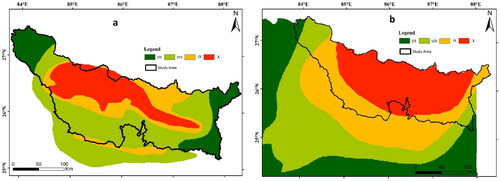The MMI values were put in Equations (4)(4) $$\mathit{MMI}=a+b\times \log \left(\mathit{PGV}\right)$$(4) and (5)(5) $$\mathrm{LSI}\mathrm{}=\mathrm{}{\text{groundwater*groundwater}}_w+{\text{Geomorphology*Geom}}_w+\text{Drainage buffer}{\text{*DF}}_W+{\text{age od deposits*age of deposits}}_w+{\text{Soil Texture*Soil Texture}}_w+{\text{structures density*structure density}}_w/\sum w$$(5) , and the PGA and PGV values were obtained for the study area for both the earthquake. Figure 3a, b shows the MMI intensity map of earthquakes 1934 8.2 and 1988 6.9 Mw.

Figure 3. Modified Mercallie Intensity map shown for 1934 earthquake (a) Modified after Kayal. (2010), and 1988 earthquake (b) Modified after GSI., 1993, Prajapati et al. (2017).

The intensity of an earthquake is influenced by soil properties; in loose soil, the observed amplification is significant when compared to rocky terrain (Zaman and Warnitchai 2017). Shear wave estimates helps with soil property analysis; in the developing countries like India, where shear wave measurements are limited or non-existent on a regional scale, Wald and Allen (2007) proposed a technique to estimate shear wave in the upper 30 m of soil for hazard analysis. The Northwest portion of the study area is red, indicating a strong S wave velocity. The location is located in the Himalayan Siwalik mountains, where the slope is steep and the accompanying shear wave runs from 700 to 900 m/s. The majority of the study area is in the plain region, where slope values range from 180 to 300, indicating the area in green color.

3.2. Liquefaction susceptibility map preparation using the multi-criteria decision-making technique (AHP)

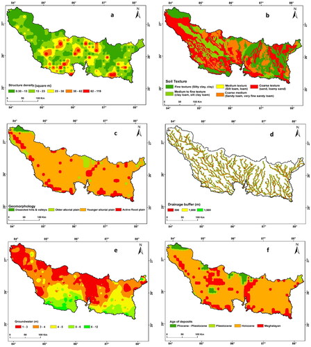
Analytical hierarchy process (AHP) was used to create a susceptibility map using six thematic layers indicated in Table 1: groundwater, structure density, soil texture, drainage buffer, age of deposits and geomorphology. The susceptibility map was then combined with a PGA layer to generate the final hazard map. Groundwater data were obtained from the Central Ground Water Board’s online portal, while geological data such as structures, age of deposits and geomorphology were obtained from BHUKOSH, the Geological Survey of India’s online portal. The NBSS Nagpur provided the soil texture data used in the study. Since the soil texture data were on printed maps at a scale of 1:5,00,000, the maps were scanned and digitized in the ArcGIS environment. The drainage density map was created using ArcGIS 10.5's hydrology tools using SRTM 30-m resolution data. The PGA layer was also included into the susceptibility map, and the final liquefaction hazard map for the study area was generated.

Table 1. Thematic layers and their importance in preparing the liquefaction susceptibility map.

Thematic layer	Liquefaction susceptibility	Data source
Groundwater table	The average water table depth for soil liquefaction is 2.05 m (Hartantyo, 2006), the water table depth was classified for the degree of hazard using the classification provided in (Chung & Rogers, 2013). Soil saturated with groundwater is susceptible to liquefaction (Bozzoni et al. 2021). The range of groundwater depth was adopted is 0–1.4 (Very highly susceptible), 1.4–3.2 (moderately susceptible), 3.2 − 4.5 (moderately susceptible), 4.5 − 7.4 (low susceptibility), >7.4 (none)	Central Ground Water Board online Portal
Structure density	The structures control the circulation and storage of groundwater, and these constitute secondary porosity (Pudi et al. 2019; Takorabt et al., 2018). A site near the structures receives more energy relative to a distant location. Classification of structure density for liquefaction susceptibility map was done using natural break application of ArcGIS. The range was distributed such as 13 (low susceptibility) > 23 (moderate susceptibility) > 38 (moderate susceptibility)> 62 (highly susceptible)> 119 (very highly susceptible)	BHUKOSH (GSI)
Soil texture	Sandy and loamy soils have relatively better water infiltration rates 20-30 mm/hr than clay-rich soils 1-10 mm/hr https://www.fao.org/3/s8684e/ s8684e0a.htm. Soil texture classification suggested in (https://www. geospatialworld.net/article/the-study-for-assessment-of-susceptibility-to-soil- liquefaction-in-taiwan/) was used in this study. The soil texture divided into coarse texture (Very highly susceptible ), medium coarse texture (highly susceptible), medium texture (moderate susceptibility), medium fine texture (moderate susceptibility), fine clay silt (Low susceptibility)	NBSS, Nagpur
Drainage buffer	Liquefaction is generally observed along the drainage (Zhu et al. 2015, 2017; Pudi et al. 2019; Bozzoni et al. 2021). The drainage buffer classified as 0–500 m from the drainage liquefaction likely, 500–1000 m liquefaction possible, and >1000 liquefaction not likely	SRTM DEM, 30m USGS
Age of deposits	Liquefaction susceptibility decreases as the alluvial and flood plains’ geologic age increases (Dobry, 1985). Meghalayan deposits are the recent deposits less than age < 10,000 yrs hence least compacted and susceptible to liquefaction. In this study, the age of deposits classified as Pliocene-Pleistocene (very low susceptibility), pleistocene (low susceptibility), Holocene (moderate susceptibility) and Meghalayan (highly susceptible). Recent deposits are common along rivers, so the drainage buffer is essential for liquefaction estimation.	BHUKOSH (GSI)
Geomorphology	Geomorphological units in the study area classified as dissected hills & valleys (very low susceptibility), piedmont slope (low susceptibility), older alluvial plain (moderate susceptibility), younger alluvial plain (highly susceptible) and active flood plain (very high susceptible)	BHUKOSH (GSI)

3.4. AHP model

AHP is a multi-criteria decision-making technique that assists the user in developing a preference scale from a collection of alternatives (Yalcin 2008). AHP is a theory of measurement dealing with quantifiable and intangible criteria applied to different decision-making problems (Vargas 1990). AHP breaks complex decision-making problems in the hierarchy of alternatives (Kumar and Anbalagan 2016). The relative importance of each parameter was given by considering the published literature and expert advice. In the first step, a pairwise comparison matrix was prepared in Table 2 by ranking the parameters from 1 to 9, where 1, 3, 5, 7, and 9 stands for equally, moderately, strongly, very strongly, extremely important and 2, 4, 6, and 8 show the compensation between odd ranks (Saaty 1990).

Table 2. Pairwise comparison matrix for site-specific parameters used to prepare the liquefaction susceptibility map.

	Groundwater	Structure density	Soil texture	Drainage buffer	Age of deposits	Geomorphology	Eigen Vector
Groundwater	1	2	3	4	4	5	0.35
Structure density	0.5	1	3	4	5	5	0.28
Soil texture	0.33	0.33	1	2	3	5	0.15
Drainage buffer	0.2	0.25	0.5	1	2	3	0.09
Age of deposits	0.25	0.2	0.33	0.5	1	2	0.06
Geomorphology	0.2	0.2	0.25	0.33	0.5	1	0.04
Total	2.48	3.98	8.08	11.83	15.5	21

Note: This analysis estimates the highest weightage 0.34 for groundwater and the lowest weightage 0.04 for geomorphology.

The rank assigned to different thematic layers are shown in Table 2; rank was given from 1 to 5 for error matrix calculation, the equal importance assumed groundwater and structure, then soil texture was slightly less important than drainage buffer and age of deposits assigned the same weightage and geomorphology allocated the 5 ratings least important relatively. Theme attributes rates were not assigned according to the AHP process; the thematic layers were reclassified from 1 to 5 hazard classes according to the details provided in Table 1.

Matrix calculation gives the weight of each parameter; also, consistency index (CI) and consistency ratio was calculated in the method to show the consistency of the decision-maker’s judgment during the evaluation. The maximum eigenvalue is also determined in this process. The expression for CI is (4) $$\mathrm{CI}\mathrm{}=\mathrm{}\frac{{\lambda }_{\mathit{max}}-N}{N-1},$$(4) where ${\lambda }_{\mathit{max}}$ is the principal eigenvalue, and N is the order of the judgment matrix. The value of CI should be less than 0.1. Consistency ratio (CR) can be calculated by the ratio CR/RI, where RI is a random index (Saaty 1990). Table 2 represents the comparison matrix for the site-specific parameters and their weightage to prepare a liquefaction susceptibility map.

The calculated weight for parameters is 0.35 for groundwater, 0.28 for structure density, 0.15 for soil texture, 0.09 for drainage buffer, 0.06 for the age of deposits, and 0.04 for geomorphology. The consistency ratio evaluated for the analysis was 0.05, which is less than 0.1. The next step is calculating the Liquefaction Susceptibility Index (LSI). GIS layers prepared in the ArcGIS 10.5 were integrated using the raster calculator tool by multiplying the raster layer and the corresponding weight of the layer. (5) $$\mathrm{LSI}\mathrm{}=\mathrm{}{\text{groundwater*groundwater}}_w+{\text{Geomorphology*Geom}}_w+\text{Drainage buffer}{\text{*DF}}_W+{\text{age od deposits*age of deposits}}_w+{\text{Soil Texture*Soil Texture}}_w+{\text{structures density*structure density}}_w/\sum w$$(5) where LSI is the liquefaction susceptibility index, and w is the weight of the individual layer.

3.5. Liquefaction hazard map

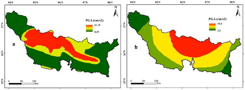
The liquefaction susceptibility map prepared in the previous step has been integrated with the PGA map. The MMI map presented in Figure 3 has been converted in the PGA Figure 6 and PGV Figure 4e, f using the simple regression relationship proposed by (Anbazhagan et al., 2016) (Figure 5). (7) $$\text{Liquefaction hazard}=\mathrm{}\sqrt{\text{Peak Ground Acceleration}\times \text{Liquefaction Susceptibility Index}}.$$(7)

Figure 4. Input layers used for liquefaction susceptibility evaluation using rapid response and loss estimation model (Zhu et al. 2017), (a) precipitation, (b) groundwater, (c) distance to water body, (d) shear wave, (e) PGV 1934, and (f) PGV 1988.

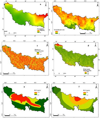
Figure 5. Input thematic layers used in the AHP model are (a) structure density, (b) soil texture, (c) geomorphology, (d) drainage buffer, (e) groundwater and (f) age of deposits. The GIS layers were scaled according to the degree of the liquefaction.

The PGA values acquired were interpolated for the study area, and a GIS layer for the PGA created is displayed in Figure 6a and b. To construct the final hazard map, the geometric mean of the PGA layer and the susceptibility map was determined using the AHP approach.

Figure 6. The PGA map prepared from the isoseismal map a) 1934 earthquake event 8.2 Mw (Kayal 2010) and (b) 1988, 6.9 Mw (Mukarjee and Lavania 1998). The PGA is in cm/sec². It is observed from the map that for 1934 high PGA values were observed than the 1988 event.

4. Results and discussion

The soil liquefaction scenario was reconstructed for the earthquakes in 1934 and 1988. The liquefaction damage scenario for both occurrences is shown in Figure 7a–d. The areas along the drainages have been indicated as high liquefaction zones on the Model A map, which displays the amount of liquefaction in percentage terms. The results revealed a strong correlation between both models (A and B) and the reference liquefaction sites, including Sitamarhi, Madhubani, Purnia and East Champaran, which were badly impacted by the earthquake. Model B also revealed a high zone around Patna and Munger, where high PGA values were found and significant liquefaction was reported. For the 1934 earthquake, the study area was categorized as very low (8%), low (48%), high (24%) and severe (20%).

Figure 7. (a, b) shows the liquefaction damage scenario during the 1934 earthquake using Model A and Model B, and (c, d) shows the liquefaction scenario during 1988 by model A and model B, respectively. The maps were classified into four zones such as very low, low, high and severe using a natural break in ArcGIS 10.5.

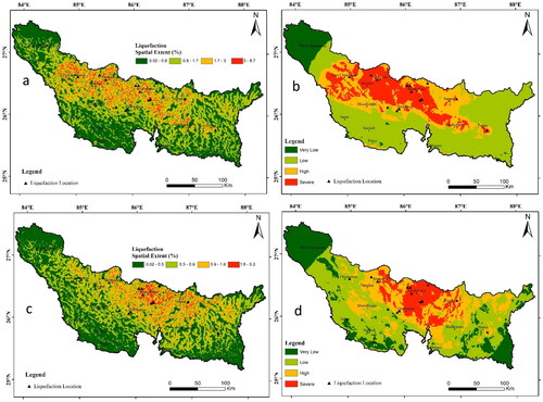
The 1988 earthquake hazard maps reveal significant liquefaction in the Madhubani, Sitamarhi, and Supaul areas where liquefaction records were discovered. The liquefaction damage intensity was found to be lower in this earthquake, implying that groundmotion factors are important in amplifying the liquefaction. The study area has been classified as Very low (23%), Low (36%), High (27%) and Severe (14%). The liquefaction hazard map produced with Model B yields data that match the Model A. The validation and comparison analysis is given in the next part to assess the accuracy of the models.

4.1. Validation

According to liquefaction reports from the 1934 earthquakes, events such as sand water geysers, ground fissuring, and sand boils were observed in Motihari, Muzaffarpur, Darbhanga, East Champaran, Madhubani, Saharsa and Purnea (Arya and Mishra 2013), which are located in the study area’s central and western regions.

Northern Bihar experienced several liquefaction events during the 1934 and 1988 earthquakes. The liquefaction has been reported in various published literature and field reports used as reference locations to validate the maps. Rajendran et al. (2016) have identified five liquefaction sites after trenching in selected sites in Northern Bihar. Sukhija et al. (2002) have identified six sites, where liquefaction was observed during past earthquake events: Narkatiya, Senvariya, Benibad, Kalikapur, Balwatola, and Tintolia. The validation included a few other sites such as Darbhanga jail, Taralahi, Sitamarhi, Purnia, Laheriasarai and Jhanjarpur.

4.2. Rmse calculation

The Root Mean Square Error (RMSE) is defined as the square root of the total of the squared differences between the categorized and reference data sets (Dehghan and Ghassemian 2006). The lower the RMSE, the more accurate the categorization (Bostanci and Bostanci 2013). The pixel values for the reference locations were extracted from the individual map prepared for both the events, and mean value was calculated. For 1934 and 1988 occurrences, the mean for reference pixels in Models A and B was estimated as 1.91, 1.18, 0.48 and 0.48. The RMSE was determined for each individual class (very low, low, high and severe) and listed in Table 3. The study revealed that the RMSE value for class ‘High’ is the lowest of all classes, implying that liquefaction locations were highly correlated with class ‘High’.

Table 3. RMSE determined for separate classes (very low, low, high and severe) in the liquefaction hazard map from the reference location.

	RMSE
Classes	1934 Model A	1934 Model B	1988 Model A	1988 Model B
Very low	1.21	0.38	0.76	0.26
Low	0.32	0.15	0.33	0.13
High	0.19	0.05	0.05	0.03
Severe	1.51	0.22	1.22	0.08

Notes: The RMSE describes how close the predicted value with the reference value. The ‘high’ class of the AHP model has the lowest RMSE value than other classes, which infers that the predicted liquefaction high zone is close to the reference liquefaction zone.

4.3. ROC analysis

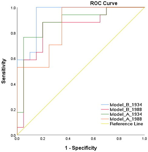
The receiver operating characteristics (ROC) curve was used to assess the models’ classification performance. The curve depicts the relationship between the true positive rate (Sensitivity) and false-positive rate (1-Specificity) (Sur et al. 2020). The model output was validated using past liquefaction manifestation locations described in the literature. The false-positive rate (FPR) is represented on the X-axis, while the true positive rate (TPR) is represented on the Y-axis. Finally, the area under curve (AUC) was calculated, it indicates the model comparison, with values ranging from 0.5 to 1. The greater the AUC, the more accurate the model (Wang et al. 2017).

The estimated AUC shown in Figure 8 for Model A was 0.88 and 0.85, while for Model B is 0.94 and 0.84 for the events 1934 and 1988, respectively. According to the AUC classification, the accuracy obtained for the 1934 earthquake using Model B is very good and good for Model B 1988 and both events of Model A.

Figure 8. The ROC curve generated using the SPSS tool shown for 1934 and 1988 earthquake for both models (a, b) the highest AUC found 0.94 for 1934 earthquake using Model B.

The liquefaction hazard is a catastrophic earthquake-induced secondary effect. The work is relevant in the today’s hazard assessment situation, when several geological hazards are considered concurrently. The approach may be used with various secondary impacts such as landslides, debris flows, floods and structural damage to assess the entire damage potential scenario in a location. Thus, decision makers may estimate the region where response planning is necessary by incorporating the secondary impacts of earthquakes or other occurrences. The study’s hazard maps may be used by urban planners to ensure that the city does not develop in the direction of a severe liquefaction zone.

5. Conclusion

The study indicates that liquefaction hazard maps created using Model B may also be used for previous earthquakes to examine damage patterns, and the information can be utilized to predict future hazards. Although spatial liquefaction maps lack precision and field-based testing are accurate, such maps and methodology will be beneficial for large area mapping and may be utilized as reconnaissance map and land demarcation tool prior to field-based surveys. In the future, the accuracy of the liquefaction susceptibility map may be improved by include litholog data, and the Probabilistic Seismic Hazard Assessment for the study region may be done to estimate the future scenario of liquefaction hazard.

Data availability statement

The data used to support the findings in this study will be available by the corresponding author upon reasonable request. Restrictions are applied to data, such as Soil Texture which is not freely available.

Disclosure statement

No potential conflict of interest was reported by the author(s).

References

- Ambraseys NN, Douglas J. 2004. Magnitude calibration of north Indian earthquakes. Geophys J Int. 159(1):165–206.
- Anbazhagan P, 2016. Relationship between intensity and recorded ground-motion and spectral parameters for the Himalayan region. Bull Seismol Soc Am. 106(4):1672–1689.
- Anbazhagan P, Bajaj K, Patel S. 2015. Seismic hazard maps and spectrum for Patna considering region-specific seismotectonic parameters. Nat Haz. 78(2):1163–1195.
- Andrus, RD, Kenneth HS. 2000. Liquefaction resistance of soils from shear-wave velocity. J Geotech Geoenviron Eng. 126(11):1015–1026.
- Arya AS, Mishra B. K. 2013. Damage scenario under hypothetical recurrence of 1934 earthquake intensities in various districts in Bihar.
- Banghar AR. 1991. Mechanism solution of Nepal-Bihar earthquake of August 20, 1988. J Geol Soc India 37:25–30.
- Baruah S, D’Amico S, Saikia S, Gautam J, Devi RK, Boruah G, Sharma A, Abdelwahed M. 2018. Study of fault plane solutions and stress drop using local broadband network data: The 2011 sikkim himalaya earthquake of mw 6.9 and its aftershocks. Ann Geophys. 61(1).
- Bilham R, et al. 1998. Geodetic constraints on the translation and deformation of India: Implications for future great Himalayan earthquakes. Curr Sci. 74:213–229.
- Bostanci B, Bostanci E. 2013. An evaluation of classification algorithms using McNemar’s test. in Proceedings of Seventh International Conference on Bio-Inspired Computing: Theories and Applications (BIC-TA 2012), p. 15–26.
- Bozzoni F, Bonì R, Conca D, Lai CG, Zuccolo E, Meisina C. 2021. Megazonation of earthquake-induced soil liquefaction hazard in continental Europe. Bull Earthq Eng. 19(10):4059–4082.
- Campbell KW, Bozorgnia Y. 2010. A ground motion prediction equation for the horizontal component of cumulative absolute velocity (CAV) based on the PEER-NGA strong motion database. Earthq Spectra. 26(3):635–650.
- Chen W-P, Molnar P. 1977. Seismic moments of major earthquakes and the average rate of slip in central Asia. J Geophys Res. 82(20):2945–2969.
- Chousianitis K, Del Gaudio V, Pierri P, Tselentis G-A. 2018. Regional ground-motion prediction equations for amplitude-, frequency response-, and duration-based parameters for G reece. Earthq Eng Struct Dyn. 47(11):2252–2274.
- Chung, Jae-Won, J. David Rogers. 2013. Influence of assumed groundwater depth on mapping liquefaction potential. Environ Eng Geosci. 19(4):377–389.
- Dasgupta S, Mukhopadhyay M, Nandy DR. 1987. Active transverse features in the central portion of the Himalaya. Tectonophysics. 136(3/4):255–264.
- Dehghan H, Ghassemian H. 2006. Measurement of uncertainty by the entropy: application to the classification of MSS data. Int J Remote Sens. 27(18):4005–4014.
- Dixit J, Dewaikar DM, Jangid RS. 2012. Assessment of liquefaction potential index for Mumbai city. Nat Hazards Earth Syst Sci. 12(9):2759–2768.
- Dobry, R. 1985. Liquefaction of soils during earthquakes, national research council (nrc), committee on earthquake engineering. Washington (DC): National Academy Press. Report No. CETS-EE-001.
- Dunn JA, et al. 1939. The Bihar–Nepal earthquake of 1934. Mem. Geol Surv India. 73:118–137.
- Fick SE, Hijmans RJ. 2017. WorldClim 2: new 1-km spatial resolution climate surfaces for global land areas. Int J Climatol. 37(12):4302–4315.
- Foulser-Piggott R, Goda K. 2015. Ground-motion prediction models for arias intensity and cumulative absolute velocity for Japanese earthquakes considering single- station sigma and within-event spatial correlation. Bull Seismol Soc Am. 105(4):1903–1918.
- Ganapathy GP, Rajawat AS. 2012. Evaluation of liquefaction potential hazard of Chennai city, India: Using geological and geomorphological characteristics. Nat Hazards. 64(2):1717–1729.
- Gupta MK. 1994. Liquefaction during 1988 earthquakes and a case study. Proceedings third international conference on case histories in geotechnical engineering, University of Missouri, Rolla, USA.
- Hartantyo, Eddy, S. K. 2014. Brotopuspito. Correlation of shallow groundwater levels with the liquefaction occurrence cause by May 2006 earthquake in the south volcanic‐clastic sediments Yogyakarta, Indonesia. Int J Appl Sci. 1:1–8.
- Iwasaki T, Arakawa T, Tokida KI. 1984. Simplified procedures for assessing soil liquefaction during earthquakes. Int J Soil Dyn Earthq Eng. 3(1):49–58.
- Karpouza M, Chousianitis K, Bathrellos GD, Skilodimou HD, Kaviris G, Antonarakou A. 2021. Hazard zonation mapping of earthquake-induced secondary effects using spatial multi-criteria analysis. Nat Hazards. 109(1):637–669. Springer Netherlands.
- Kayal JR. 2001. Microearthquake activity in some parts of the Himalaya and the tectonic model. Tectonophysics. 339(3/4):331–351.
- Kayal JR. 2010. Himalayan tectonic model and the great earthquakes: an appraisal. Geom Nat Haz Risk. 1(1):51–67.
- Kayal JR. 2014. Seismotectonics of the great and large earthquakes in Himalaya. Curr Sci. 106(2):188–197.
- Keshri CK, Mohanty WK, Ranjan P. 2020. Probabilistic seismic hazard assessment for some parts of the Indo-Gangetic plains, India. Nat Haz. 103(1):815–843.
- Kumar R, Anbalagan R. 2016. Landslide susceptibility mapping using analytical hierarchy process (AHP) in Tehri reservoir rim region, Uttarakhand. J Geol Soc India. 87(3):271–286.
- Mar M. 1991. Geotechnical damage due to Bihar earthquake of August 1988.
- Mohindra R, Parkash B, Prasad J. 1992. Historical geomorphology and pedology of the Gandak Megafan, Middle Gangetic Plains, India. Earth Surf Process Landforms. 17(7):643–662.
- Molnar P, Pandey MR. 1989. Rupture zones of great earthquakes in the Himalayan region. J Earth Syst Sci. 98(1):61–70.
- Mukarjee S, Lavania BVK. 1998. Soil Liquefaction in Nepal-Bihar Earthquake of August 21, 1988. International Conference on Case Histories in Geotechnical Engineering. 11:587–592. http://scholarsmine.mst.edu/icchge/4icchge/4icchge-session03/11.
- Mukhopadhyay M. 1984. Seismotectonics of transverse lineaments in the eastern Himalaya and its foredeep. Tectonophysics. 109(3/4):227–240.
- Naik SP, Patra NR, Malik JN. 2022. Cyclic behavior of late quaternary alluvial soil along Indo-Gangetic Plain: Northern India. Geo-Eng. 13(1):1–20.
- Nath SK, Adhikari MD, Maiti SK, Ghatak C. 2019. Earthquake hazard potential of Indo-Gangetic Foredeep: its seismotectonism, hazard, and damage modeling for the cities of Patna, Lucknow, and Varanasi. J Seismol. 23(4):725–769.
- Nath SK, Srivastava N, Ghatak C, Adhikari MD, Ghosh A, Sinha Ray SP. 2018. Earthquake induced liquefaction hazard, probability and risk assessment in the city of Kolkata, India: its historical perspective and deterministic scenario. J Seismol. 22(1):35–68.
- Nath SK, Thingbaijam KKS. 2012. Probabilistic seismic hazard assessment of India. Seismol Res Lett. 83(1):135–149.
- Philip G, Suresh N, Bhakuni SS. 2014. Active tectonics in the northwestern outer Himalaya: Evidence of large-magnitude palaeoearthquakes in pinjaur dun and the frontal Himalaya. Curr Sci. 106(2):211–222.
- Prajapati, Sanjay K., Harendra K. Dadhich, Sumer Chopra. 2017. Isoseismal map of the 2015 Nepal earthquake and its relationships with ground-motion parameters, distance and magnitude. J Asian Earth Sci. 133:24–37.
- Pudi R, Martha TR, Roy P, Vinod Kumar K, Rama Rao P. 2019. Regional liquefaction susceptibility mapping in the Himalayas using geospatial data and AHP technique. Curr Sci. 116(11):1868–1877.
- Putti SP, Satyam N. 2018. Ground response analysis and liquefaction hazard assessment for Vishakhapatnam city. Innov Infrastruct Sol. 3(1):1–14.
- Rajendran CP, John B, Rajendran K, Sanwal J. 2016. Liquefaction record of the great 1934 earthquake predecessors from the north Bihar alluvial plains of India. J Seismol. 20(3):733–745.
- Rao KS, Satyam DN. 2007. Liquefaction studies for seismic microzon of Delhi region, 92(5):646–654.
- Rathje EM, Abrahamson NA, Bray JD. 1998. Simplified frequency content estimates of earthquake ground motions. J Geotech Geoenviron Eng. 124(2):150–159.
- Richter CF. 1958. Elementary seismology. San Francisco, CA: W.H. Freeman and Company.
- Robertson PK, Wride CE. 1996. Cyclic liquefaction and its evaluation based on SPT and CPT: Summary Report. NCEER Workshop on Evaluation of Liquefaction Resistance of Soils (January 1997), pp. 41–88. https://www.cpt-robertson.com/PublicationsPDF/NCEERsummary.pdf.
- Saaty TL. 1990. How to make a decision: the analytic hierarchy process. Eur J Oper Res. 48(1):9–26.
- Sapkota SN, Bollinger L, Klinger Y, Tapponnier P, Gaudemer Y, Tiwari D. 2013. Primary surface ruptures of the great Himalayan earthquakes in 1934 and 1255. Nature Geosci. 6(1):71–76.
- Sapkota SN, Bollinger L, Perrier F. 2016. Fatality rates of the M w ∼8.2, 1934, Bihar-Nepal earthquake and comparison with the April 2015 Gorkha earthquake 4. Seismology the 2015 Gorkha, Nepal, Earthquake and Himalayan Studies: First Results. Earth Planets Space. 68(1)1–9.
- Satyam N. 2012. Review on liquefaction hazard assessment. In: Moustafa A, editor. Advances in geotechnical earthquake engineering–soil liquefaction and seismic safety of dams and monuments. Intech-Open.
- Seeber L, Armbruster JG. 1981. Earthquakes along the Himalayan arc quaternary and reworked tertiary J folding thrusting. Earthq Pred: Int Rev. 4:259–277.
- Seed HB, Idriss IM. 1971. Simplified procedure for evaluating soil liquefaction potential. J Soil Mech and Found Div. 97(9):1249–1273.
- Singh DD, Gupta HK. 1980. Source dynamics of two great earthquakes of the Indian subcontinent: The Bihar-Nepal earthquake of January 15, 1934 and the Quetta earthquake of May 30, 1935. Bullet Seismol Soc Am. 70(3):757–773.
- Sitharam TG, Kumar A, Anbazhagan P. 2013. Comprehensive seismic microzonation of Lucknow city with detailed geotechnical and deep site response studies. Proceedings of Indian Geotechnical Conference, December, pp. 1–21.
- Sukhija BS, et al. 2002. Palaeoliquefaction evidence of prehistoric large/great earthquakes in North Bihar, India. Curr Sci. 83(8):1019–1025.
- Sur U, Singh P, Meena SR. 2020. Landslide susceptibility assessment in a lesser Himalayan road corridor (India) applying fuzzy AHP technique and earth-observation data. Geomatics Nat Hazards Risk. 11(1):2176–2209.
- Takorabt, Mebarka, et al. 2018. Determining the role of lineaments in underground hydrodynamics using Landsat 7 ETM + data, case of the Chott El Gharbi Basin (western Algeria). Arab J Geosci. 11(4):1–19.
- Valdiya KS. 2016. Indo-Gangetic plains: Evolution and later developments (Goswami 1985). In: Valdiya KS, editor. The making of India. Cham: Springer; p. 723–745.
- Vargas LG. 1990. An overview of the analytic hierarchy process and its applications. Eur J Oper Res. 48(1):2–8.
- Verma AK, Pati P, Sharma V. 2017. Soft sediment deformation associated with the East Patna Fault south of the Ganga River, northern India: influence of the Himalayan tectonics on the southern Ganga plain. J Asian Earth Sci. 143:109–121.
- Verma M, Bansal BK. 2013. Active fault mapping: an initiative towards seismic hazard assessment in India. J Geol Soc India. 82(2):103–106.
- Wald DJ, Allen TI. 2007. Topographic slope as a proxy for seismic site conditions and amplification. Bull Seismol Soc Am. 97(5):1379–1395.
- Wang F, Xu P, Wang C, Wang N, Jiang N. 2017. Application of a GIS-based slope unit method for landslide susceptibility mapping along the Longzi River, southeastern Tibetan Plateau, China. IJGI. 6(6):172.
- Wood, Harry O., Frank Neumann. 1931. Modified Mercalli intensity scale of 1931. Bull Seismol Soc Am. 21(4):277–283.
- Yalcin A. 2008. GIS-based landslide susceptibility mapping using analytical hierarchy process and bivariate statistics in Ardesen (Turkey): Comparisons of results and confirmations. Catena. 72(1):1–12.
- Youd TL, Hoose SN. 1977. Liquefaction susceptibility and geologic setting. The 6th World Conference on Earthquake Engineering, p. 2189–2194.
- Youd TL, Idriss IM, Andrus RD, Arango I, Castro G, Christian JT, Dobry R, Finn WDL, Harder LF, Hynes ME, et al. 2001. Liquefaction Resistance of Soils: Summary Report from the 1996 NCEER and 1998 NCEER/NSF Workshops on Evaluation of Liquefaction Resistance of Soils. J Geotech Geoenviron Eng. 127(10):817–833.
- Zaman S, Warnitchai P. 2017. Topographically-derived near-surface shear wave velocity map for Pakistan. J Earthq Tsunami. 11(02):1650010.
- Zhu J, Baise LG, Thompson EM. 2017. An updated geospatial liquefaction model for global application. Bull Seismol Soc Am. 107(3):1365–1385.