Spatiotemporal analysis of monthly rainfall over Saudi Arabia and global teleconnections

Abstract

This research focuses on extracting the statistical features, in space and time, of the monthly rainfall in Saudi Arabia (SA) and the relation to the large-scale atmospheric variability through teleconnection for strategic water resources planning. These features are useful for future predictions. 28 stations distributed over SA for a period between 1970 and 2012 are utilized. According to the Kolmogorov–Smirnov (K-S) test, the Log-normal and Gamma distributions are dominant, while for the Chi-squared (Chi2) test, the Beta distribution is dominant. The K-S is preferable since it works with the original data rather than the Chi² that uses binning, and therefore, some information is lost. The L-moment analysis showed that Person type III is dominant for the wet season while there is no obvious distribution for the dry season. Empirical Orthogonal Function (EOF) analysis is applied to seasonal rainfall data for studying the dominant modes of climate variability and associated large-scale circulation patterns. Our results demonstrate a robust relationship between the wet season (November – April) with El Niño Southern Oscillation (ENSO) and Pacific Decadal Oscillation (PDO), whereas the dry season (June – September) is associated with the Indian Ocean Dipole (IOD). Moreover, the warm (cold) phase of PDO is associated with excess (deficit) rainfall, indicating some predictability of the seasonal rainfall over SA.

Keywords:

• Monthly rainfall
• statistical analysis
• empirical orthogonal function
• teleconnections

1. Introduction

Water resources in arid and semi-arid regions are suffering from scarcity. Governmental organizations are seeking an evaluation of the existing water resources in each country and seeking predictions of the future of water resources for strategic planning. Saudi Arabia (SA) is one of those countries. Therefore, the current study is focusing on the evaluation of the monthly rainfall pattern in space and time, as the main and natural fresh surface water resource in the country. The analysis is based on the available historical data (from the local ground rainfall stations and the global climate variability perspective). This, in turn, will help in developing realistic models for future predictions of rainfall in space and time.

For annual rainfall analysis over SA, Mashat and Abdel Basset (2011) studied rainfall using data from 28 stations distributed over SA in the period from 1970 up to 2003. The analysis focused on homogeneity tests (Bartlett 1937) of the stations. They concluded that the mean annual rainfall depth seems to be homogeneous at a 95% confidence level except at the Tabuk and Sharorah stations (Mitchell et al. 1966). The mean annual rainfall depth at the Jouf and Abha stations (in the southern part of SA) indicates some in-homogeneities. The highest amount of rainfall occurs during spring over the southwest, middle, and east of SA. Elfeki et al. (2013) studied the annual rainfall variability at some stations in SA. The study used the variance (power) spectrum density function to find out the frequency component that produces the peak variance in the data. Their study concluded that although the structural pattern of the variance is complicated due to the high degree of variability in the rainfall, there is a dominant 25-year cycle in the studied stations.

For monthly rainfall analysis, Alyamani and Sen (1993) used 29 stations over SA for 15 years of record to study the monthly rainfall data. They concluded that the monthly rainfall depth is almost log-normally distributed; however, they did not mention the type of statistical test they used in the analysis. However, in the current study, strict statistical tests are performed to test the rainfall distributions. Elfeki and Al-Amri (2011) modeled monthly rainfall time series using a two-state Markov chain (dry and wet months). However, it was limited to only three stations that do not represent the rainfall condition of SA as a whole. They also assumed that the Markov chain is homogenous which is not the case. The current study does not focus on the monthly time series in a sequential form however, it considers an in-depth statistical analysis of the monthly variability of rainfall over space and time from rainfall stations and the link to large-scale atmospheric variability through teleconnection to get a complete picture of the monthly and seasonal variability over SA and develop, in the future, a non-homogeneous monthly time series model for rainfall data.

For daily and sub-daily data, several studies dealt with daily rainfall and the development of intensity-duration-frequency (IDF) curves for the hydrological design (Al-Shaikh 1985, Al-Saleh 1994, Al-Hassoun 2011, Elsebaie 2012, Al-Anazi and El-Sebaie 2013, and Subyani and Al-Amri 2015). These studies considered some stations or some regions in SA, but the work by Ewea et al. (2017) considered SA as a whole. They developed IDF curves using the extreme value theory for stormwater design networks in the region.

Elfeki et al. (2014) analyzed the sub-daily storm data to provide the design storm pattern in each of the 13 districts in SA. These patterns are mainly useful in the hydrological applications of watersheds in the region for flood protection studies. Subyani and Hajjar (2016) studied the duration of dry and wet spells of daily rainfall series available in the period from 1971 to 2012 for the Jeddah region in the west of SA. They observed changes in the trend of the dry and wet spell durations and rainfall depths at different time scales (daily, monthly, and annual) time series. Subyani (2019) studied the spatial and temporal continuity of rainfall patterns using geostatistical models in space and time in the western part of SA. His study is based on a space-time standardized variogram to model the spatial-temporal structure of precipitation. There is a high temporal variability but low spatial variability in the studied region.

In other arid regions worldwide, there are no sufficient studies on monthly rainfall analyses. Some studies are found in Iran by Eslamian and Feizi (2007) where they used L-moment to analyze the maximum monthly rainfall in Isfahan Province. Zamani and Bazrafshan (2020) modeled the monthly rainfall data using zero-adjusted models in Iran. By this model, they were able to classify Iran into different rainfall regimes, especially for the semi-arid, arid, and extra-arid regions. Adnan et al. (2017) used monthly data to analyze the shifting of agro-climatic zones in Pakistan. They revealed that almost 87% of Pakistan is in extremely arid to semi-arid zones. Bouklikha et al. (2021) performed an innovative trend analysis (ITA) method of the annual, seasonal, and monthly rainfall in the Tafna watershed, North West of Algeria. The monthly rainfall shows a decreasing trend in the studied stations. Seasonal analysis indicates a downward trend in winter and spring.

Atmospheric variability on monthly and longer timescales is dominated by the presence of coherent large-scale spatial patterns (Saravanan and McWilliams 1998), which play an important role in atmosphere-ocean interactions. On sub-annual to inter-annual timescales, El Niño southern oscillation (ENSO) over the tropical eastern Pacific Ocean, Pacific Decadal Oscillations (PDO), and Indian Ocean Dipole (IOD) can also play an important role in such interactions. The recurring patterns in the large-scale atmospheric circulations (North Atlantic Oscillation and North Annular Mode), moisture transportation, fluxes of heat, and atmosphere-ocean system (such as ENSO) cause diverse climate variations (Iqbal and Athar 2018). These large-scale atmospheric-oceanic circulation patterns with time scales ranging from several weeks to years and their linkages to weather and climate anomalies are typically referred to as teleconnection patterns (Hannachi et al. 2017, Yu and Lupo 2019, Hannachi 2021). These patterns are also referred to as prominent modes of low-frequency variability, where many of the patterns are also planetary-scale in nature. The structure and frequency of occurrence of these planetary-scale teleconnection patterns have also been widely studied by several investigators (Wallace and Gutzler 1981; Saravanan 1998; Latif et al. 2017).

Precipitation is one of the most important components of the climate system, whose variability is strongly coupled to the atmosphere-ocean large-scale dynamics. Precipitation variability at local to regional scales is a major challenge for agriculture production, food security, natural resource management, climate change, hydrological modeling studies, and many more (Ebert et al. 2007; Gordon et al. 2010). Changes in precipitation occurrence, intensity, frequency, and spatiotemporal variability in a changing climate are expected to increase often leading to extreme events and affecting the water balance and the ecosystem (Bastiaanssen and Ali 2003). For investigating the dependencies of precipitation in SA on the occurrence and intensity (in terms of circulation indices) of particular teleconnection patterns, the Pearson correlation coefficient has been used extensively in the meteorological literature (Syed et al. 2012; Krichak et al. 2014; Plewa et al. 2019; Syed et al. 2022).

Weather and climate vary on a wide range of spatial and temporal scales. One of the particular interests here is the effect of the so-called large-scale and low-frequency modes of climate variability. These modes, by their very own nature, have longer time scales, compared to typical synoptic scales of weather systems (few days and few thousand kilometers), and therefore can persist longer and affect remote areas. These modes of variability are known in climate literature as teleconnections. Teleconnection patterns connect weather and climate over a large distance, which persists longer than typical baroclinic timescales. Teleconnection patterns have been widely studied in the past 100 years using different ocean-atmospheric variables viz., Sea Surface Temperature (SST), Sea Level Pressure (SLP), surface air temperature, and geopotential height for different pressure levels (see, for instance, Philander 1990; Hannachi and Stendel 2016; Iqbal and Athar 2018; Aamir and Hassan 2020; Atif et al. 2020). The identification of the occurrence of teleconnection patterns is commonly applied for assessing the climate variability on time scales ranging from months to years. Examples of the most common teleconnection patterns include the North Atlantic Oscillation (NAO), ENSO, IOD, Arctic Oscillation (AO), and Pacific Decadal Oscillation (PDO). The NAO, for example, reflects a seesaw in atmospheric mass (SLP) between the Azores and Icelandic region (see, for instance, Hannachi and Stendel 2016). It is the dominant mode of atmospheric variability in the northern hemisphere (NH) winter with centers of action located in the North Atlantic region. ENSO is the largest climate teleconnection on the planet and represents primarily a coupled ocean-atmosphere phenomenon in the tropical Pacific (Philander 1990). ENSO is reflected as a change of polarity in the SST anomalies in the eastern tropical Pacific, mainly in the NH wintertime. Those teleconnections affect weather and climate remotely in many ways (e.g., Hannachi et al. 2017). So far, very few studies have investigated the association between teleconnections and precipitation in the Arabian peninsula (Athar 2015; Kumar et al. 2016; Atif et al. 2020; Syed et al. 2022). However, the spatiotemporal analysis of seasonal (dry: June – September and wet: November – April) variability of rainfall and its connection to large-scale circulation patterns has not been studied yet. Therefore, this study may provides implications for the seasonal rainfall prediction in SA.

As mentioned in the literature, the available studies focused only on describing some limited monthly data (either by choosing a few stations e.g., Elfeki and Al-Amri 2011 or by considering short records and a few statistical analyses e.g., Alyamani and Sen1993) or at different time scales (e.g., annual time scale e.g., Mashat and Abdel Basset 2011, Elfeki et al. 2013 or daily and sub-daily time scale e.g., Al-Shaikh 1985, Al-Saleh 1994, Al-Hassoun 2011, Elsebaie 2012, Al-Anazi and El-Sebaie 2013, and Subyani and Al-Amri 2015, Ewea et al. 2017).

In the current study we focused on monthly data since they are more related to climate, i.e., long-term variability, and also seasonality, both are important components for long-term planning. The analysis is done systematically for the first time herein and combined with both a detailed statistical analysis of the monthly and seasonal rainfall data and the link to large-scale atmospheric variability through teleconnection patterns since these issues are not yet considered in climate studies in SA.

Therefore, the objectives of this study can be summarized as:

• Develop a detailed statistical analysis of the available monthly rainfall stations that are distributed across SA and the extraction of the statistical measures and probability distributions (based on various statistical tests: Chi² test, Kolmogorov–Smirnov test, and L-moments) to analyze the monthly rainfall variability in space and time. This will help in developing predictions of monthly rainfall in the future for water resources evaluation, strategic planning, and developing downscaling to a finer time scale.

• Examine the influence of large-scale circulation indices, i.e. ENSO, PDO, and IOD (also referred to as the Dipole Mode Index, DMI), on seasonal (dry and wet) rainfall in SA using Empirical Orthogonal Function (EOF) technique to get the common spatial patterns of variability and temporal projections of the associated patterns. The extracted rainfall features are especially useful to analyze the climatic variability in SA for future predictions of rainfall and consequently provide a reliable estimation of the surface water resources in the region.

The organization of the paper is as follows: Section 2 describes the data collection. Section 3 describes the methodology. Section 4 presents the results of the analysis, and the conclusion is given in the last section.

2. Data description

Monthly rainfall data are collected from the available 28 meteorological stations distributed over SA and managed by the General Meteorological Organization. The rainfall data covered the temporal period 1970 − 2012, but with different starting dates for different stations. The analysis was performed based on the available record for each station. This is the best one can do. In general, and worldwide there are always stations with different record lengths and researchers have to cope with the available record length.

Detailed information, including the number of storms for each station, is presented in Table 1. The distribution of the stations is uneven in the different provinces (Figure 1). Figure 2 shows the maximum, average, and standard deviation of the monthly rainfall depth along with the 90%, 95%, and 99% percentiles. It is obvious from the graph that June, July, and August are dry months for 17 stations. The rest of the stations (11 stations) has rainfall over the year-round with a high degree of variability. The maximum monthly rainfall depth (513.8 mm) is observed in Turaif in February 1980. The second maximum value is observed in Abha (415.2 mm) in March 1997. The third maximum value is observed in Jeddah (258.2 mm) in November 1995. The rest of the stations have maxima less than 250 mm (Figure 1).

Figure 1. Rainfall stations used in the study area.

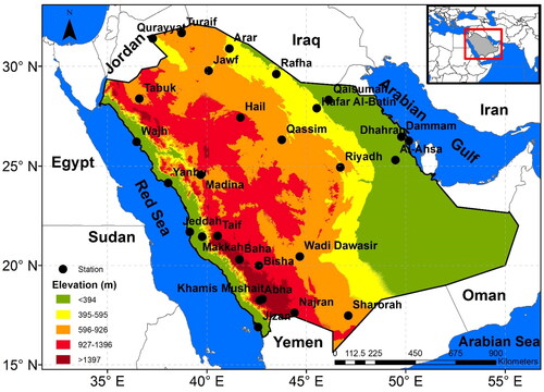
Figure 2. Maximum, mean, and standard deviation of monthly rainfall depth for the stations in the current study with 90%, 95% and 99% percentiles.

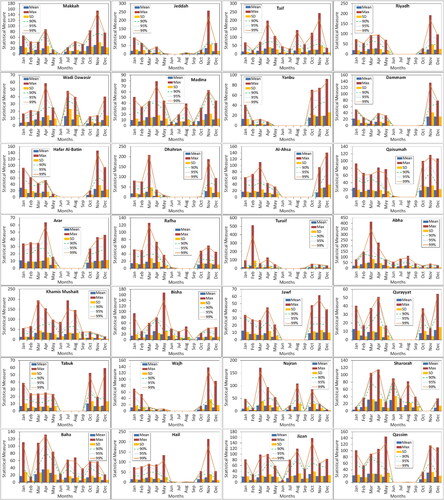
Table 1. Rainfall stations were used in the current study.

Z. NO.	Zone	Station number	Station name	Recorded storms		Coordinates		Total number of storms
				From	To	Longitude	Latitude
1	Makkah	41030	Makkah	1985	2012	39°46′08″	21°26′16″	392
		41024	Jeddah	1970	2012	39°08′54″	21°40′42″	317
		41036	Taif	1970	2012	40°32′56″	21°28′44″	1278
2	Riyadh	40437	Riyadh	1985	2012	46°43′19″	24°55′31″	691
		41061	Wadi Dawasir	1978	2012	44°40′49″	20°26′30″	350
3	Madina	40430	Madina	1970	2012	39°41′55″	24°32′53″	589
		40439	Yanbu	1978	2012	38°03′50″	24°08′24″	184
4	Eastern Region	40417	Dammam	1999	2012	49°46′59″	26°27′59″	323
		40377	Hafar Al-Batin	1990	2012	45°32′00″	27°54′00″	578
		40416	Dhahran	1970	2012	50°09′39″	26°15′34″	1216
		40420	Alahsa	1985	2012	49°29′11″	25°17′53″	644
		40373	Qaisumah	1978	2012	46°07′49″	28°19′08″	1203
5	Northern Borders	40357	Arar	1979	2012	41°08′26″	30°54′08″	752
		40362	Rafha	1978	2012	43°29′49″	29°37′17″	973
		40356	Turaif	1978	2012	38°44′22″	31°41′16″	1028
6	Asir	41112	Abha	1978	2012	42°39′39″	18°13′59″	1729
		41114	Khamis Mushait	1970	2012	42°48′23″	18°17′58″	1726
		41084	Bisha	1970	2012	42°37′09″	19°59′28″	943
7	Al-Jouf	40361	Jawf	1978	2012	40°05′55″	29°47′19″	673
		40360	Qurayyat	1985	2012	37°16′56″	31°24′27″	645
8	Tabuk	40375	Tabuk	1978	2012	36°36′25″	28°22′35″	501
		40400	Wajh	1978	2012	36°28′37″	26°12′19″	288
9	Najran	41128	Najran	1978	2012	44°24′49″	17°36′41″	497
		41136	Sharorah	1985	2012	47°06′29″	17°28′04″	228
10	Baha	41055	Baha	1985	2012	41°38′35″	20°17′41″	972
11	Hail	40394	Hail	1970	2012	41°41′28″	27°26′04″	1047
12	Jizan	41140	Jizan	1970	2012	42°35′05″	16°53′49″	556
13	Qassim	40405	Qassim	1978	2012	43°46′03″	26°18′28″	1037

To examine the spatiotemporal behavior of seasonal (dry: June – September and wet: November – April) rainfall variability, the 28-years (1985 − 2012) rainfall data of 27 meteorological stations are analyzed in association with the large-scale flow. Note that the Dammam station has been excluded from the list of 28 stations (Table 1), as it does not cover the whole study period. The data of monthly large-scale climatic indices (ENSO, PDO, and IOD) were obtained from Climate Explorer website (https://climexp.knmi.nl/selectindex.cgi). For ENSO index, the Niño 3, Niño 3.4, and Niño 4 data was used. The PDO (Kennedy et al. 2011) is a robust pattern of climate variability, defined by the leading principlal component of monthly SST variability in the extratropical north Pacific ocean (Mantua et al. 1997). It is characterized by positive (warm) and negative (cold) phases. During a warm (cold) phase, the west Pacific becomes more cooler (warmer) and part of eastern ocean warms (cools) (Wu 2013). The IOD is an irregular oscillation of SST, defined as the difference between western equatorial Indian ocean (10°S − 10°N latitude and 50°E − 70°E longitude) and south-eastern equatorial Indian Ocean (10°S − 0°N latitude and 90°E − 110°E longitude) SST anomalies (°C). During a positive (negative) phase, the eastern Indian ocean cools (warms) and part of western Indian ocean warms (cools). In this study, the circulation indices data sets for ENSO and IOD are based on HadISST1, whereas PDO is constructed based on HadSST3 product.

For analyzing the large-scale teleconnection patterns, associated with seasonal rainfall variability in the region, the monthly global mean Hadley Centre Sea Ice and Sea Surface Temperature (HadISST) SST data (Rayner et al. 2003) provided by the Hadley Centre, with a horizontal resolution of 1 degree × 1 degree, for the period 1985 − 2012 are used in this study.

3. Methodology

The methodology of this study can be divided into two parts: The first part is to derive the statistical measure of the monthly rainfall characteristics in space and time and obtain the best probability distribution that fits the monthly data per station based on Chi² and K-S tests for future predations of monthly rainfall. In the second part, we endeavor to investigate the linkage of seasonal rainfall with large-scale teleconnection patterns. The detail of the methodology is presented below.

Several statistical characteristics have been estimated from the data, namely: the monthly mean (µ), standard deviation (σ), coefficient of variation (CV), and skewness (γ). Some of these descriptors are shown below. Some monthly rainfall probability density functions (pdf) have been tested namely, the normal distribution, log-normal distribution, exponential distribution, gamma distribution, beta distribution, and Gumbel distribution (Table 2). The method of moments is used to estimate the parameters of each distribution (Kite 1978).

Table 2. The common pdfs, f(x), used in the analysis.

Distribution	Pdf formula	Pdf Parameters
		$\mu$	${\sigma }^2$
Normal	$f\left(x\right)=\frac{1}{\beta \sqrt{2\Pi }}{e}^{-\frac{1}{2{\beta }^2}{(x-\alpha )}^2}$-∞ < x < ∞	$\alpha$	${\beta }^2$
Log-Normal	$f\left(x\right)=\frac{1}{x\beta \sqrt{2\Pi }}{e}^{-\frac{1}{2{\beta }^2}{(\mathit{Lnx}-\alpha )}^2}$x > 0	$\alpha$	${\beta }^2$
Exponential	$f\left(x\right)=\frac{1}{\alpha }{e}^{-\alpha x}\alpha$>0,x > 0	$\frac{1}{\alpha }$	$\frac{1}{{\alpha }^2}$
Gamma	$f\left(x\right)=\frac{1}{\Gamma (\alpha )}{x}^{\alpha -1}{e}^{-(\frac{x}{\beta })}\alpha$ ,β > 0,x > 0	$\alpha \beta$	${\alpha \beta }^2$
Beta	$f\left(x\right)=\frac{\Gamma \left(\alpha \right)+\Gamma (\beta )}{\Gamma (\alpha )\Gamma (\beta )}{x}^{\alpha -1}{(1-x)}^{\beta -1}\alpha$ ,β > 0,x > 0	$\frac{\alpha }{\alpha +\beta }$	$\alpha \beta /{\left(\alpha +\beta \right)}^2\left(\alpha +\beta +1\right)$
Gumbel	$f\left(x\right)=\frac{1}{\beta }{e}^{\left[-\left(\frac{x-\alpha }{\beta }\right)e^{-\left(\frac{x-\alpha }{\beta }\right)}\right]}$-∞ < x < ∞	$\alpha +0.5772\beta$	$\frac{{\pi }^2}{6}{\beta }^2$

Two tests are considered, namely the Kolmogorov–Smirnov (K-S) test (Kolmogorov 1933, Smirnov 1933) and the Chi-square test (Greenwood and Nikulin 1996). The K-S test is applied to unbinned data to compare the cumulative distribution of the data against a specified null distribution:

$$H_{°}:\mathrm{}{x}_i\text{is distributed as the specified distribution}.$$$$H_1:\mathrm{}{x}_i\text{is not distributed as the specified distribution}.$$

where H_o is the null hypothesis,

H₁ is the alternative hypothesis, and

$x_i$ is the random variable that represents the monthly rainfall depth.

If the K-S test, given by Eq. (6)(6) $$K\_S={\max }_{i=1,\dots ,n}\left|F\left(x_i,\theta \right)-F_n\left(x_i\right)\right|$$(6) , (6) $$K\_S={\max }_{i=1,\dots ,n}\left|F\left(x_i,\theta \right)-F_n\left(x_i\right)\right|$$(6) where, $F\left(x_i,\theta \right)$ is the theoretical distribution function with parameters$\theta ,$ and

$F_n\left(x_i\right)$is the empirical cumulative distribution function (CDF),

is greater than the tabular value, then the null hypothesis is rejected at a given level of significance, α has been taken to be 5%. The best out of these distributions is the one with the minimum value of the test (Kite 1978).

The Chi-Squared test (${\chi }^2$) is also used and is based on binned data, and the number of bins (k) is defined as, (7) $$k\mathrm{}=\mathrm{}1\mathrm{}+\mathrm{}\log \left(2n\right)\mathrm{}$$(7) where n is the sample size, and the test is given by, (8) $${\chi }^2=\frac{\sum _{i=1}^{i=k}{(O_i-E_i)}^2}{E_i}$$(8) where O_i is the observed frequency from the data, and E_i is the expected frequency from the specified distribution for bin i.

The K-S test is generally preferred because binning the data takes away some information. However, in the current study, both tests are used to show the effect of the test on the choice of the distribution. The statistical descriptors are mapped using the geographical information system (GIS) technique based on the kriging method to analyze their variation in space and time.

L-moment analysis is also performed to analyze the regional trend in the data. The L-moment method used is explained in detail in Hosking (1990). A summary is given here. The L-moment ratios for the L-skewness coefficient, ${\tau }_3,$ and L-kurtosis coefficient, ${\tau }_4,$are given by, (9) $${\tau }_3=\frac{l_3}{l_2},\mathrm{}\mathit{and}\mathrm{}{\tau }_4=\frac{l_4}{l_2}$$(9) where, l₂, l₃, and l₄ are the sample L-moments for the second, third, and fourth months which are given by linear combinations of the product moments as, (10) $${l_2=2b}_1-b_0\mathrm{}$$(10) (11) $${l_3=6b_2-6b}_1+b_0\mathrm{}$$(11) (12) $${l_4=20b_3-30b_2+12b}_1-b_0\mathrm{}$$(12) where (13) $$b_r=\frac{1}{n}\sum _{i=1}^n{x}_i.{F\left(x_i\right)}^r,\mathrm{}r=1,\dots \mathrm{}$$(13) where x_i should be in ascending order, n is the number of data points, and the F(x_i) is the non-exceedance probability which can be estimated by the plotting position formula (Hosking 1990), (14) $$F\left(x_i\right)=\frac{i-0.35}{n}$$(14) where i is the rank of the data in ascending order.

The L-moments ratios in Equation 9(9) $${\tau }_3=\frac{l_3}{l_2},\mathrm{}\mathit{and}\mathrm{}{\tau }_4=\frac{l_4}{l_2}$$(9) are then compared with the L-moment ratio diagram presented by Hosking (1990) to define the suitable distribution of the data for regional trend analysis in the discussion section.

In the second part of this study, we applied an Empirical Orthogonal Function (EOF) analysis (Hannachi et al. 2007) on detrended seasonal rainfall anomalies for studying the spatiotemporal behavior of rainfall variability as well as its linkage to global teleconnections. EOF analysis is the most widely used statistical technique in climate research to determine the dominant spatial patterns of variability. Dominant modes of variability are usually given by the leading EOFs, i.e., the eigenvectors of the covariance matrix of the data, and the corresponding amplitudes in time (or principal component, PC, time series). The leading EOF and associated time series explain the maximum variance of the analyzed field. To identify the dominant (large-scale) teleconnection associated with a local climate process, such as rainfall in Arabia in this case, we first identified the dominant mode of variability (seasonal) of regional precipitation. The obtained time series (principal component, PC) of the leading precipitation EOF is then correlated with the global SST anomalies at each grid point.

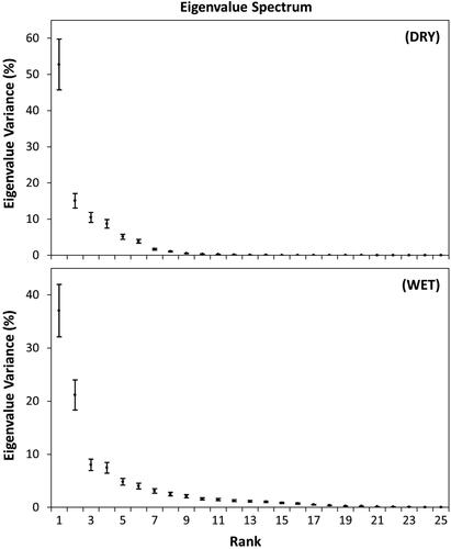
Monthly rainfall data of 27 meteorological stations are used covering 28 years (1985 − 2012) time period. In this study, only the first Principal Component (PC1) is taken into consideration, as it explains the largest fraction of the variance of the data. We calculated the uncertainties on the leading EOFs to further support our argument that the leading mode is separated from rest of the spectrum (Figure 3). The Pearson correlation coefficient (r) is used to measure the strength of a linear relationship between leading PC1 of rainfall and different circulation indices [ENSO (Niño 1.2, Niño 3, Niño 3.4, and Niño 4), Bivariate ENSO Timeseries (BEST), NAO, IOD, AO, and PDO] with α set to a 5% significance level. Only those indices which showed the statistical significance with PC1 (rainfall) have been selected for the analysis. The obtained large-scale map is then compared to documented teleconnection maps. The monthly data of circulation indices were averaged to obtain the values of dry and wet seasons.

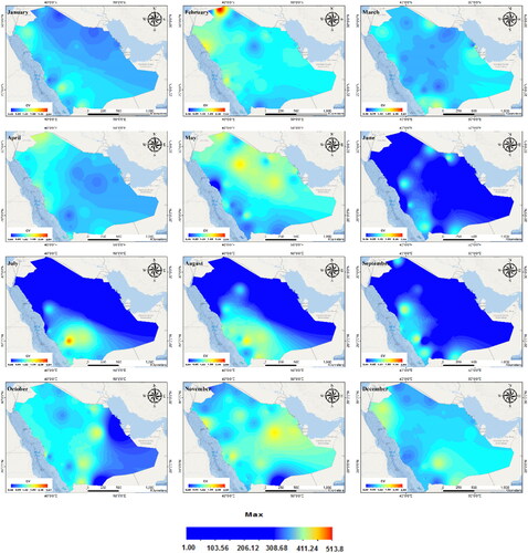
Figure 3. Spatiotemporal distribution of the maximum monthly rainfall depth for the stations in the current study from January to December.

To further substantiate the linkage of rainfall with ENSO and PDO, composites of SST and rainfall anomalies for wet season is discussed. In order to define the above-normal and below-normal phases, the SST climate indices are standardized. For ENSO cycle, the El Niño (warm phase) events are determined based on the criterion that the standardized seasonal (wet) Niño 3.4 index is ≥ to 0.5, whereas the La Niño (cold phase) events are identified when standardized Niño 3.4 index is ≤ to −0.5. Similarly, PDO cycles are defined following Kiem et al. (2003) as the standardized seasonal PDO index ≥ 0.5 is considered as the positive (warm) phase of PDO, whereas the negative (cold) phase of PDO is defined when the seasonal PDO index is ≤ −0.5, and neutral when PDO index lies between −0.5 and 0.5.

4. Analysis of the results

4.1. Statistical indicators

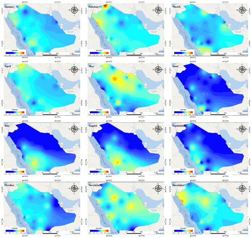
The results of the study are displayed in various maps and graphs to provide an interpretation of the spatiotemporal rainfall pattern, namely; the maximum (Figure 3), the median (Figure 4) monthly rainfall, addition to the coefficient of variation (Figure 5), and the skewness coefficient (Figure 6).

Figure 4. Spatiotemporal distribution of the median of the monthly rainfall depth for the stations in the current study from January to December.

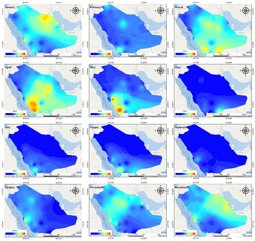
Figure 5. Spatiotemporal distribution of the monthly coefficient of variation (CV) for the stations in the current study from January to December.

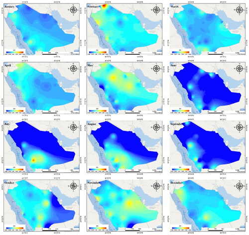
Figure 6. Spatiotemporal distribution of the monthly skewness for the stations in the current study from January to December.

In January (Figure 3), the rainfall region between 75 to 150 mm is located in the southwest, east, and north of the country. The remaining area has a rainfall of less than 75 mm. February corresponds to the largest amount of rainfall in comparison with other months, with maximum values ranging between 150 and 510 mm, located in the Al-Jouf region. In March, the maximum rainfall ranges between 150 mm and 440 mm, located in the southwestern part, while the middle and the eastern regions have maximum rainfall that ranges between 75 mm and 150 mm. The north and western parts have maximum rainfall of less than 75 mm. In April and May, the maximum rainfall ranges between 160 mm and 220 mm and is located in the southwestern part. The eastern and northern parts have maximum rainfall of less than 75 mm. In Jun the maximum is in general less than 75 mm. July and August are similar to June, except that the maximum rainfall is ranging between 75 and 150 mm in the southwest. September and October show the lowest maximum rainfall. November shows the location of maximum rainfall in the west spots with rainfall values ranging between 230 to 290 mm, while rainfall depth between 160 mm to 220 mm is located in the mid-west. Most of the region has maximum rainfall between 75 and 150 mm. December has a maximum rainfall of less than 75 mm, located in the middle and eastern parts of the region. The above results indicate the seasons and the geographic locations that are expected to flood and drought and therefore, assist in developing measures for resource management.

The median (Figure 4) ranges from 0.1 mm to 31 mm. The maximum median is located in the southwest in April, May, September, and October. The coefficient of variation, CV, (Figure 5) varies between 0.1 and 2.8. This indicates a significant variation in CV. The highest value of CV is located in the north in February whereas the lowest CV is in June, July, August, and September in the north, northwestern and eastern parts of the country. The skewness (Figure 6) varies between 0.19 and 5.2. This indicates a tendency toward low rainfall depths, which is typical for arid regions. The figure shows significant changes in the skewness over the months. The spatial patterns of the skewness are similar to those of CV. The highest value of skewness is located in the north during February. While the lowest is in June, July, August, and September in the north, northwest, and east of SA.

This observed variability from the previous figures is attributed to the topography of the region. The western part of the region has a chain of mountains along the Red Sea coast which is a key player in the climate regime in the region (Alyamani and Sen 1993).

Table 3 summarizes the upper and lower limits of the statistical descriptors of the monthly rainfall. Turaif has the highest rainfall, standard deviation, CV, and skewness γ in February. The maximum average monthly is 51.75 mm at Abha station in March, while the minimum is 0.63 mm at Qassim in August. The minimum standard deviation (0.30) and CV (0.48) are located at Qassim in August. The maximum median is observed in Najran in June. The sign of the skewness is positive which means that the distribution is skewed to the left towards the low rainfall regime. The maximum coefficient of kurtosis is located in Turaif station in February and the minimum in Wajh in May.

Table 3. Summary statistics.

Statistical descriptor	Value	Station name	Month	Year
Max	513.80 (mm)	Turaif	Feb	1980
Min	0.10 (mm)	Many Stations
Average Max	51.75 (mm)	Abha	Mar
Average Min	0.63 (mm)	Qassim	Aug
SD Max	92.47 (mm)	Turaif	Feb
SD Min	0.30 (mm)	Qassim	Aug
CV Max	2.84	Turaif	Feb
CV Min	0.48	Qassim	Aug
Median Max	45.05 (mm)	Najran	Jun
Median Min	0.10 (mm)	Many Stations
Skew Max	5.2	Turaif	Feb
Skew Min	0.03	Dhahran	Oct
Kurt max	27.8	Turaif	Feb
Kurt min	2.1	Wajh	May

Figure 7 is a sample station result that compares the theoretical CDF and the empirical probability distribution of Taif’s monthly rainfall. The best distribution, based on the K-S test, varies from month to month. In the case of Taif station, as shown in Table 4, the best distributions for January to December are respectively, Beta, Log-normal, Beta, Gamma, Beta, Log-normal, Exponential, Gamma, Gamma, Gamma, Log-normal, and Exponential. It is obvious from these distributions that the summer months (August, September, and October) have the same distribution (Gamma). The non-uniformity in the type of distribution of the stations over the months makes it difficult to provide future predictions using time series analysis. A non-stationary and non-homogenous time-series analysis should be used in this case to model such variability.

Figure 7. Comparison between the theoretical CDF and the empirical probability distribution of Taif monthly rainfall.

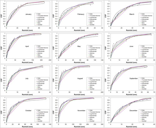
Table 4. Results of the K-S test for the rainfall distributions over the stations and the months of the year.

Station		Jan	Feb	Mar	Apr	May	Jun	Jul	Aug	Sep	Oct	Nov	Dec
Name	Number
Makkah	41030	Beta	LogNor	Beta	Gam	Gam	–	LogNor	LogNor	Gam	Beta	Gam	Beta
Jeddah	41024	LogNor	LogNor	Gam	LogNor	LogNor	–	–	Gam	Gam	Gam	LogNor	Beta
Taif	41036	Beta	LogNor	Beta	Gam	Beta	LogNor	Exp	Gam	Gam	Gam	LogNor	Exp
Riyadh	40437	Gum	LogNor	Gam	Gam	LogNor	–	–	–	–	LogNor	LogNor	Beta
Wadi Dawasir	41061	Beta	LogNor	Beta	Gam	LogNor	–	LogNor	LogNor	–	LogNor	Gam	LogNor
Madina	40430	LogNor	Gam	Gum	Gam	LogNor	LogNor	Gam	Gam	LogNor	Beta	Gam	Gum
Yanbu	40439	Gum	LogNor	LogNor	LogNor	–	–	–	–	–	Gam	Gam	LogNor
Dammam	40417	Nor	Gum	Beta	Beta	LogNor	–	–	–	–	–	Beta	Beta
Hafar Al-Batin	40377	Gam	LogNor	LogNor	Gam	LogNor	–	–	–	–	LogNor	Gam	Exp
Dhahran	40416	Gam	Gam	Non	Gam	Exp	–	–	–	–	Nor	Gam	Beta
Al-Ahsa	40420	Beta	LogNor	Beta	Beta	Gum	–	–	–	–	–	Gam	Gam
Qaisumah	40373	Gum	LogNor	Gam	LogNor	LogNor	Gam	–	–	–	LogNor	Beta	Beta
Arar	40357	Gam	Beta	Beta	Gam	LogNor	–	–	–	–	Gam	Gam	LogNor
Rafha	40362	Beta	LogNor	Gam	LogNor	LogNor	Gum	–	–	–	Gam	Gam	Beta
Turaif	40356	Exp	LogNor	Gam	Beta	LogNor	–	–	–	LogNor	Exp	Beta	Beta
Abha	41112	LogNor	Gam	LogNor	Gam	Beta	Beta	LogNor	Beta	LogNor	Beta	Gam	Beta
Khamis Mushait	41114	Gam	Gum	LogNor	Beta	Beta	LogNor	Gam	Exp	Gam	LogNor	LogNor	Beta
Bisha	41084	Gam	Beta	Beta	Beta	Exp	LogNor	LogNor	LogNor	–	Gum	Beta	LogNor
Jawf	40361	Beta	Beta	Beta	Gam	Gam	–	–	–	–	Gam	Gam	Exp
Qurayyat	40360	Exp	Gum	LogNor	LogNor	Gam	–	–	–	–	Gam	Beta	Gam
Tabuk	40375	LogNor	LogNor	LogNor	Gam	LogNor	–	–	Gam	–	LogNor	Beta	LogNor
Wajh	40400	Exp	LogNor	LogNor	LogNor	LogNor	–	–	–	–	Gum	LogNor	LogNor
Najran	41128	LogNor	Gum	LogNor	Gam	LogNor	–	Gam	LogNor	–	LogNor	LogNor	Beta
Sharorah	41136	Gam	Exp	Beta	LogNor	Beta	Gum	LogNor	Gam	LogNor	–	–	LogNor
Baha	41055	Gam	Gam	LogNor	Beta	Gam	LogNor	Gam	Gam	LogNor	LogNor	Gum	Beta
Hail	40394	Beta	Gam	Gam	Non	LogNor	Nor	–	LogNor	Gam	Gum	Gam	Gam
Jizan	41140	Beta	Beta	Gam	Gam	Beta	LogNor	LogNor	LogNor	Gam	Gam	Nor	LogNor
Qassim	40405	Gam	Beta	Exp	Exp	LogNor	–	–	Gam	–	Gam	Beta	Gam

(-) No enough data for statistical analysis (less than or equal 3 values), (LogNor) is lognormal, (Nor) is normal, (Exp) is exponential, (Gam) is Gamma, (Gum) is Gumbel, (Beta) is Beta, and (Non) none of the distributions fits the data.

Figure 8 is similar to Figure 7 but for Abha station and the results of the Chi-square test. The distributions (Table 5) for January to December are Beta, None, Log-normal, Beta, None, Log-normal, None, Beta, None, Beta, Beta, and Beta respectively. Note that none of the proposed distributions fitted February, May, July, and September. This makes it difficult to provide reliable predictions in these months at Abha station and therefore, another statistical measure should be considered such as the L-moment analysis given below.

Figure 8. Sample of the comparison between the theoretical frequency histogram and the frequency histogram of the data for Chi² test: Abha station from January to December.

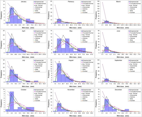
Table 5. Results of the Chi-square test for the rainfall distributions over the stations and the months of the year.

Station		Jan	Feb	Mar	Apr	May	Jun	Jul	Aug	Sep	Oct	Nov	Dec
Name	Number
Makkah	41030	Non	Beta	Beta	Non	Beta	–	Nor	Beta	Beta	Beta	Beta	Non
Jeddah	41024	Non	Non	Beta	Beta	Beta	–	–	Beta	Nor	Beta	Non	Non
Taif	41036	Beta	Non	Beta	Beta	Beta	Beta	Beta	LogNor	Non	Beta	Non	Beta
Riyadh	40437	Beta	Beta	Beta	Beta	Non	–	–	–	–	Beta	Non	Beta
Wadi Dawasir	41061	Beta	Beta	Non	Beta	Non	–	Nor	Beta	–	Beta	Beta	Beta
Madina	40430	Beta	Beta	Non	Beta	Beta	Beta	Beta	Beta	Beta	Beta	Non	Beta
Yanbu	40439	Non	Beta	Beta	Beta	–	–	–	–	–	Beta	Beta	Beta
Dammam	40417	Nor	Beta	Nor	Beta	Beta	–	–	–	–	–	Beta	Non
Hafar Al-Batin	40377	Beta	Non	Beta	Non	Non	–	–	–	–	Beta	Beta	Beta
Dhahran	40416	Beta	Non	Non	Beta	Beta	–	–	–	–	Nor	Beta	Beta
Al-Ahsa	40420	Beta	Beta	Beta	Beta	Beta	–	–	–	–	–	Beta	Beta
Qaisumah	40373	Beta	Beta	Beta	Beta	Non	Nor	–	–	–	Beta	Beta	Beta
Arar	40357	Beta	Beta	Non	Beta	Beta	–	–	–	–	Beta	Beta	Beta
Rafha	40362	Beta	Beta	Beta	Beta	Non	Nor	–	–	–	Beta	Beta	Beta
Turaif	40356	Beta	Non	Beta	Non	Non	–	–	–	Non	Beta	Beta	Non
Abha	41112	Beta	Non	LogNor	Beta	Non	LogNor	Non	Beta	Non	Beta	Beta	Beta
Khamis Mushait	41114	Beta	Beta	Non	Beta	Beta	LogNor	Beta	Beta	Beta	Beta	Beta	Beta
Bisha	41084	Beta	Beta	Beta	Non	Non	Non	Non	Non	–	Nor	Non	Beta
Jawf	40361	Beta	Beta	Beta	Non	Beta	–	–	–	–	Beta	Beta	Beta
Qurayyat	40360	Beta	Beta	Beta	Non	Beta	–	–	–	–	Beta	Nor	Non
Tabuk	40375	Non	Non	Beta	Beta	Non	–	–	Beta	–	Beta	Beta	Non
Wajh	40400	LogNor	Non	Beta	Beta	Nor	–	–	–	–	Beta	Non	Non
Najran	41128	Non	Beta	Non	Beta	Beta	–	Beta	Non	–	Beta	Beta	Nor
Sharorah	41136	Beta	Beta	Beta	Non	Nor	Nor	Beta	Beta	Beta	–	–	Beta
Baha	41055	Beta	Beta	Beta	Beta	Beta	Non	Beta	Non	Beta	Non	Beta	Beta
Hail	40394	Beta	Beta	Beta	Beta	Non	Nor	–	Nor	Beta	Beta	Non	Beta
Jizan	41140	Beta	Beta	Beta	Beta	Beta	Non	Beta	Beta	Beta	Beta	Beta	Non
Qassim	40405	Beta	Beta	Non	Beta	LogNor	–	–	Nor	–	Non	Beta	Non

(-) No enough data for statistical analysis (less than or equal 3 values), (LogNor) is lognormal, (Nor) is normal, (Exp) is exponential, (Gam) is Gamma, (Gum) is Gumbel, (Beta) is Beta, and (Non) none of the distributions fits the data.

Tables 4 and 5 show the results of both K-S and Chi-square tests, respectively. It is obvious from Table 4 that the best CDF varies from month to month with no specific pattern. It also varies over the stations. However, Table 5 shows that most of the distributions are beta. This makes it easy to use one probability model for future predictions. However, the effect of binning in the Chi-square test may not be reliable since information can be lost during the binning process.

Table 6 shows the percentage (over stations) of the best-fitted distributions for each month based on the K-S test. The table shows that Gamma and Beta constitute the maximum percentages (28.6% each) in January. For February, the Log-normal distribution is the highest (46.4%). March shows that Log-normal and Beta are dominant whereas the Gamma distribution is dominant in April (46.4%). In May, June, and July, the Log-normal distribution is dominant (55.6%, 54.5%, and 54.5% respectively). For August, September, October, and November, the Gamma is dominant (46.7%, 54.5%, 36%, and 44.4% respectively). Beta is dominant in December (42.9%). It is also worth mentioning that the Normal and Gumbel are not appropriate, most probably because of their respective zero and negative skewness.

Table 6. Percentage of the fitting distributions based on K-S test of the twelve months for KSA stations.

Distribution	Jan	Feb	Mar	Apr	May	Jun	Jul	Aug	Sep	Oct	Nov	Dec
Normal	3.6	0.0	0.0	0.0	0.0	9.1	0.0	0.0	0.0	4.0	3.7	0.0
Log-normal	17.9	46.4	32.1	25.0	55.6	54.5	54.5	40.0	45.5	32.0	22.2	28.6
Exponential	10.7	3.6	3.6	3.6	7.4	0.0	9.1	6.7	0.0	4.0	0.0	10.7
Gamma	28.6	17.9	25.0	46.4	14.8	9.1	36.4	46.7	54.5	36.0	44.4	14.3
Beta	28.6	17.9	32.1	21.4	18.5	9.1	0.0	6.7	0.0	12.0	25.9	42.9
Gumbel	10.7	14.3	3.6	0.0	3.7	18.2	0.0	0.0	0.0	12.0	3.7	3.6
None	0.0	0.0	3.6	3.6	0.0	0.0	0.0	0.0	0.0	0.0	0.0	0.0

Bold italics represents the maximum percentage of the fitted distribution for each month.

Table 7 shows the percentage of the best-fitted distributions for each month based on the Chi-square test over all stations. The table shows that Beta distribution is dominant for all months (the percentage varies between 51.9% in May to 84% in October) except June, where Normal distribution is dominant (36.4%). It should also be mentioned that the non-fitting distributions in the test are quite high, it ranges between (8% in October to 37% in May). The exponential and Gamma do not fit any data.

Table 7. Percentage of the fitting distributions based on Chi² test of the 12 months for KSA stations.

Distribution	Jan	Feb	Mar	Apr	May	Jun	Jul	Aug	Sep	Oct	Nov	Dec
Normal	3.7	0.0	3.6	0.0	7.4	36.4	18.2	13.3	9.1	8.0	3.7	3.7
Log-normal	3.7	0.0	3.6	0.0	3.7	18.2	0.0	6.7	0.0	0.0	0.0	0.0
Exponential	0.0	0.0	0.0	0.0	0.0	0.0	0.0	0.0	0.0	0.0	0.0	0.0
Gamma	0.0	0.0	0.0	0.0	0.0	0.0	0.0	0.0	0.0	0.0	0.0	0.0
Beta	77.8	71.4	67.9	77.8	51.9	18.2	63.6	60.0	63.6	84.0	70.4	66.7
Gumbel	0.0	0.0	0.0	0.0	0.0	0.0	0.0	0.0	0.0	0.0	0.0	0.0
None	14.8	28.6	25.0	22.2	37.0	27.3	18.2	20.0	27.3	8.0	25.9	29.6

Bold italics represents the max percentage of the fitted distribution for each month.

Table 8 displays a comparison of both the K-S and Chi-square tests for all the months. The Log-normal and Gamma distributions are dominant in the results based on the K-S test. They provide 35.2% and 30% respectively. However, based on the Chi-square test the Beta distribution is the highest with 67.9%.

Table 8. Summary of the test statistics over KSA stations for the 12 months.

Distribution	K-S test	Chi^2 test
Normal	1.5%	6.5%
Log-normal	35.2%	2.3%
Exponential	5.2%	0.0%
Gamma	30.0%	0.0%
Beta	21.3%	67.9%
Gumbel	6.0%	0.0%
None	0.7%	23.3%

Figure 9a shows the L-moment diagram for L-skewness (L-Skew) and L-kurtosis (L-Kurt) ratios. Image (a) in the figure shows the dry season for all stations. The points are scattered and show different distributions (Person type III, generalized Pareto, and Log-normal) however the majority of the points are out of the regions of the distributions between the Pearson type III and the overall lower bound. However, for the wet season in image (b), the data in the overall stations seems to follow generalized extreme value as an upper boundary, Person type III, Log-normal, generalized logistic, and generalized Pareto. Image (c) shows the average over the 12 months for the 28 stations. Most of the data lie between the Patriot distribution and the overall lower bound. There is no obvious probability distribution since the data is averaged over the 12 months. However, for image (d), where the average is performed over all stations for each month, there is an obvious probability distribution for the wet season (January, February, March, April, May, November, and December) which is Person type III while there is no obvious probability distribution for the dry months (June, July, August, September, and October). This might be due to data scarcity in these months.

Figure 9 . a. L-moment diagram for L-skewness (L-Skew) and L-kurtosis (L-Kurt) ratios: (a) dry season for all stations, (b) wet season over all stations, (c) average over all months, (d) average over all stations. Months that have data less than 3 values with the month at some stations are omitted from the figure. b. Relationship between kurtosis (Kurt) and skewness (Skew) over the months.

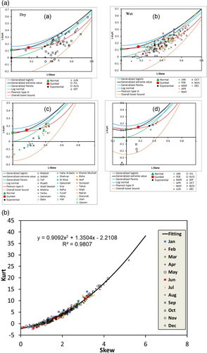
Figure 9b shows a scatter plot of the kurtosis (Kurt) versus skewness (Skew) for all the months and stations. The figure shows a kind of scaling law of the Kurt-Skew relationship for the region. A second-order polynomial provides a very good fit, with a high coefficient of determination R2 of 0.98. This result is contradictory to the study presented by Alyamani and Sen (1993) where they found a linear relationship. This might be due to the shorter time record they used in the analysis.

4.2. Link to large-scale teleconnections

The identification of the link between local processes, such as rainfall in this case, and large-scale modes of variability is very important in climate analysis. The variability of local precipitation can have remote (i.e., large-scale) and local (e.g., convective) sources. Local sources are highly variable with short-time scales and are hence difficult to predict. Large-scale teleconnections, on the other hand, have longer time scales and are hence more predictable. ENSO and NAO, for example, are frequently used as predictors in many climate studies. The identification of a large-scale teleconnection influence on a local scale process can lend predictive power to the latter. This is because large-scale teleconnections are quite predictable with a predictability time scale that can be up to several months ahead. To summarize, a large association of a local process with large-scale teleconnection can be used to gain some predictability skills of the former.

4.2.1. Empirical orthogonal function (EOF) analysis

Eigenvalue spectrum (% of the covariance matrix of seasonal rainfall with uncertainties estimates is shown is Figure 10. The uncertainties on the leading EOFs are calculated based on North’s Rule of Thumb. The figure clearly shows that the leading EOF is well-separated from rest of the eigenvalue spectrum and can be examined separately.

Figure 10. Eigenvalue spectrum (%) of the covariance matrix of rainfall for Dry (upper) and Wet (lower) seasons. The vertical bar shows the uncertainty estimates based on rule of thumb. The leadings 25 eigenvalues are shown.

In Saudi Arabia, the rainfall is mainly confined to the wet season, whereas a very little or no rainfall occurs in dry season, except for South Asian summer monsoon and topographically driven precipitation events over the southwestern parts (Hasanean and Almazroui 2015). The spatial patterns of the leading EOF mode for seasonal rainfall are shown in Figure 11. In dry season, the first EOF leading pattern (EOF1) explains 52.7% of the total variance showing uniform positive signs across the entire domain, except Al-Ahsa station in the northeastern part of the domain, indicating coherent inter-annual variations over the study area (Figure 11a). It is noted that the highest positive values are centered over the south-western part, as this region receives most of the precipitation during the dry season (Syed et al. 2019), which is linked to the northward shifting of inter Tropical Convergence Zone (ITCZ).

Figure 11. (a) Spatiotemporal distribution of the first leading mode of EOF analysis on the interannual variation of June – September (Dry) rainfall. (b) Same as (a), except for the Wet (November – April) season.

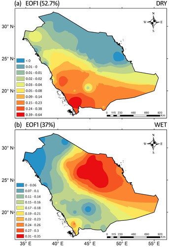
For the wet season, the first mode explains 37% of the total variance showing positive values over the whole domain, with the highest values centered over the central-eastern parts (Figure 11b) indicating that the rainfall is coupled over the whole region in wet season. Therefore, rainfall variability in this season could be governed by some large-scale phenomena. According to Syed et al. (2019), the rainfall during wet season is mainly associated with the cyclonic weather systems originated in Mediterranean Sea and advected eastward by the upper-level subtropical westerlies.

Correlations (%) between the leading (detrended) PC of the observed rainfall and SST (HadISST) anomalies (1985 − 2012) for dry and wet seasons are shown in Figure 12. It is observed that the leading PC of rainfall, related to a dry season, shows significantly negative correlation (r = −0.41) with IOD in the tropical Indian ocean, consistent with earlier work by Athar (2015). He found negative dominancy of correlation coefficient with IOD in JJA (dry) season. Moreover, Chakraborty et al. (2006) pointed out the role of atmospheric moisture flux with IOD. They reported that atmospheric moisture flux decreases (increases) during the negative (positive) phase of IOD, which supports our findings on the relationship between IOD and rainfall. The time series of PC1 of rainfall and IOD index is shown in Figure 13a.

Figure 12. (a & b) Correlation (%) of detrended PC1 of rainfall with SST (HadISST) for Dry (JJAS) and Wet (NDJFMA) seasons, respectively for the period 1985 – 2012. The dotted regions show values at 5% significance level.

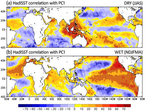
Figure 13. (a) Time series of PC1 of rainfall for dry season over KSA and the average Dipole Mode Index (DMI) during 1985 – 2012. (b) Same as (a), except for the Niño 3, Niño 3.4, and Niño 4 indices for wet season. (c) Same as (b), except for Pacific Decadal Oscillations (PDO) index. All the values of the correlations between PC1 of rainfall and climate indices are statistically significant at 95% level.

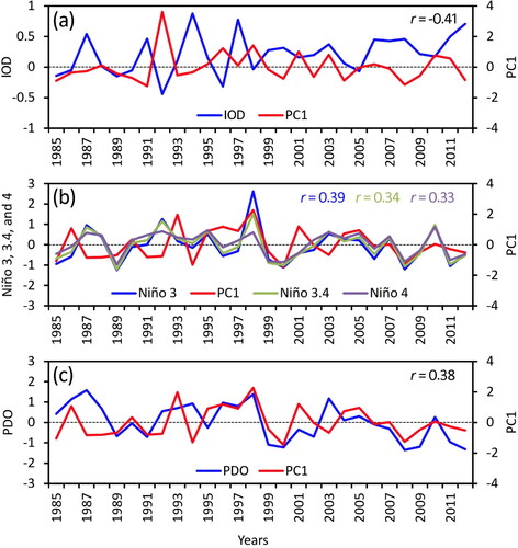
For the wet season (Figure 12b), the correlation of the first principal component (PC1) with SSTs clearly shows a positive (warm) phase of both ENSO (El Niño) in the eastern equatorial Pacific Ocean and PDO in the north Pacific ocean. The correlation between PC1 and Niño 3, Niño 3.4, Niño 4, and PDO are 0.39, 0.34, 0.33, and 0.38, respectively (Figure 13b and c). The Figure 12b further shows Interdecadal Pacific Oscillation (IPO)-like mode, i.e., positive SST anomalies in the eastern equatorial Pacific Ocean and along the west coast of North America, (Power et al. 1999; Folland et al. 2002, Christensen et al. 2013; Kirtman et al. 2013) during the wet season. However, PC1 of rainfall doesn’t show a significant correlation value (R = 0.29) with HadISST1 anomalies during the wet rainy season. The SA rainfall variations could be linked to this low-frequency climate variability mode (i.e., IPO) in the Pacific Ocean basin, as the obtained correlation value (0.29) is close to the critical value of R (0.317) in addition to the spatial pattern of IPO. Moreover, the correlation of PC1 with Bivariate ENSO Timeseries (BEST) is 0.35 (not shown). Therefore, the presented results clrealy show that the leading mode of rainfall variability for wet season in SA is significantly linked to the warm phase of both ENSO and PDO.

Figure 13 shows a comparison of time series of IOD, ENSO, and PDO indices with rainfall in the wet season. We note that the warm or positive phase of ENSO (El-Niño) and PDO corresponds to higher rainfall, whereas a cool or negative phase of both ENSO and PDO leads to a very little rainfall in SA (Figure 13b and 13c). The recent drought years (e.g., 2007, 2008, 2009, 2011, and 2012) in SA are consistent with the negative values of both PDO and El Niño indices. For details of drought episodes for the period 1985 − 2020, see Syed et al. (2022). Therefore, we may conclude that the rainfall over KSA in wet season is enhanced (suppressed) during El Niño (La Niña) phase.

4.2.2. Composites of SST and rainfall anomalies

To further substantiate the linkage and non-linear association of rainfall with ENSO and PDO, composites of SST and rainfall anomalies for wet season are presented in Figure 14. Based on the criteria for determining the positive and negative phases of ENSO and PDO (discussed in data section), the number of years included in the composite analysis of SST and rainfall anomalies for the period 1985 − 2012 are 9, 11, 10, and 9 for El Niño, La Niña, positive PDO, and negative PDO, respectively. Figure 14a displays the composite of SST anomalies during El Niño years, showing a strong positive anomalies in the central and eastern tropical pacific with a horseshoe-shaped spatial pattern, flanked by weak negative anomalies on both sides of the equator. The spatial structure of the SST composite anomalies associated with La Niña is similar to El Niño, but with opposite sign (Figure 14c). The strong negative anomalies are confined in the central Pacific. Figure 14b shows the composite of rainfall anomalies associated with the El Niño events. Clearly the El Niño or warm phase of ENSO is linked to the positive (negative) rainfall anomalies over the eastern (western) half of the country, indicating wet (dry) conditions. The La Niña composite of rainfall (Figure 14d) indicates negative anomalies over almost the whole region, indicating drought conditions.

Figure 14. (a and b) El Niño composite of SST and rainfall anomalies, respectively, for wet season. (c – d, e – f, and g – h) Same as first row, except for La Niña, Warm PDO, and Cold PDO composites, respectively. Units are degrees Celsius (°C) for SST and mm/month for rainfall.

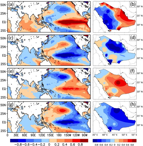
Figure 14e shows the composite of SST anomalies during warm phase of PDO. The positive anomalies along the west coast of North America wrap in a horseshoe-shaped pattern around a core of negative SST anomalies in the central part of the north Pacific. The spatial pattern of the SST composite anomalies associated with cold phase of PDO is similar to the warm phase of PDO, but with opposite sign (Figure 14g). The positive and negative PDO composites of rainfall anomalies are examined for obtaining the relationship between SST patterns and the rainfall of SA. We note that the positive PDO composite shows wet conditions (above normal rainfall) over SA (Figure 14f), whereas the negative PDO composite indicates dry conditions over the study region (Figure 14h), indicating a robust relationship between PDO and rainfall in wet season over the country.

5. Summary and conclusion

In this paper, we have investigated the monthly rainfall characteristics and the variability associated with ground station observations in Saudi Arabia (SA) for the period 1970-2012. In particular we focused our analysis on the variability of the descriptive statistics in space and time over KSA and the best pdf that fits the monthly rainfall data using several statistical tests (Chi², K-S test, and L-moment). Since the local rainfall is influenced by the large-scale ocean and atmospheric variability, therefore, we have linked the influence of large-scale climate indices with rainfall patterns in the region. The following conclusions have been drawn from this analysis:

• The skewness coefficient is positive indicating a tendency towards low rainfall depths which is a common feature in arid regions.

• The K-S and the Chi-square tests are applied with different distributions for the stations under study and at different months. The K-S statistic is preferred as a test to choose the best distribution since it works with the original data, and also because the Chi-square test uses binning, which yields a loss of information during the binning process.

• According to the K-S test, the log-normal and Gamma distributions are dominant. They fit 35.2% and 30% of the stations and over the months at a 5% significant level respectively.

• According to the Chi-square test, the Beta distribution is dominant fitting about 68% of the stations and months at a 5% significant level. The exponential distribution fits 2.3% of the stations, Gamma, and Gumbel did not fit any of the data.

• The Kurt-Skew relationship shows a kind of (universal) scaling law for all stations and all months, which can be considered a characteristic feature of the region.

• The L-moment analysis shows that Person type III is dominant for the wet season (January, February, March, April, May, November, and December) while there is no obvious probability distribution for the dry months (June, July, August, September, and October) which can be accounted for the limited data in these months.

• Our results revealed a robust association between rainfall and large-scale ocean and atmospheric climate indices such as ENSO, PDO, and IOD on seasonal (dry and wet) time scale. It is found that the positive or warm phase of PDO is significantly linked to rainfall surplus, whereas the negative or cold phase leads to rainfall deficit in wet season over the country.

• ENSO is another most dominant mode of coupled ocean-atmosphere variability causing rainfall variability in the wet season. El Niño (La Niña) phase of ENSO is associated with positive (negative) rainfall anomalies over the eastern (western) half of the country, indicating wet (dry) conditions during the wet season.

The leading mode of rainfall, associated with dry season, is negatively correlated with IOD (negative phase) in the tropical Indian ocean.

The results of this study will be followed by another research study, in the future, that incorporates the outcome to develop a non-homogeneous spatiotemporal time series model for the monthly rainfall predictions in SA and introduces downscaling from monthly to daily time scales. This is aimed at providing decision-makers with future scenarios of the water resources conditions in KSA for strategic planning.

Acknowledgment

The authors, therefore, gratefully acknowledge DSR technical and financial support.

Disclosure statement

No potential conflict of interest was reported by the author(s).

Data availability statement

The authors have no permission to submit the data since it belongs to the ministry.

Additional information

Funding

This project was funded by the Deanship of Scientific Research (DSR), King Abdulaziz University, Jeddah, under grant No. (DF-748-155-1441).

References

- Aamir E, Hassan I. 2020. The impact of climate indices on precipitation variability in Baluchistan, Pakistan. Tellus A: Dynamic Meteorol Oceanograph. 72(1):1833584.
- Adnan S, Ullah K, Gao S, Khosa AH, Wang Z. 2017. Shifting of agro-climatic zones, their drought vulnerability, and precipitation and temperature trends in Pakistan. Int J Climatol. 37(S1):529–543.
- Al-Anazi KK, El-Sebaie IH. 2013. Development of intensity-duration-frequency relationships for Abha city in Saudi Arabia. Int J Comput Eng Res. 3:2250–3005.
- Al-Hassoun SA. 2011. Developing an empirical formulae to estimate rainfall intensity in Riyadh region. J King Saud Univ–Eng Sci. 23:81–88.
- Al-Saleh MA. 1994. Frequency analysis of rainfall in Al-Quwayiyah area. Saudi Arabia. Riyadh: King Saud University. (Research Papers in Geography; no 17).
- Al-Shaikh AA. 1985. Rainfall frequency studies for Saudi Arabia. [M.Sc. thesis]. Riyadh: Civil Engineering Department, King Saud University.
- Alyamani MS, Sen Z. 1993. Reginal variation of monthly rainfall amounts in the Kingdom of Saudi Arabia. JKAU: Earth Sci. 6PI':113–133.
- Athar H. 2015. Teleconnections and variability in observed rainfall over Saudi Arabia during 1978–2010. Atmos Sci Lett. 16(3):373–379.
- Atif RM, Almazroui M, Saeed S, Abid MA, Islam MN, Ismail M. 2020. Extreme precipitation events over Saudi Arabia during the wet season and their associated teleconnections. Atmos Res. 231:104655.
- Bartlett MS. 1937. Properties of sufficiency and statistical tests. Proc Roy Stat Soc Series A 160:268–282.
- Bastiaanssen WG, Ali S. 2003. A new crop yield forecasting model based on satellite measurements applied across the Indus basin, Pakistan. Agric Ecosyst Environ. 94(3):321–340.
- Bouklikha A, Habi M, Elouissi A, Hamoudi S. 2021. Annual, seasonal and monthly rainfall trend analysis in the Tafna watershed, Algeria. Appl Water Sci. 11(4):77.
- Chakraborty A, Behera SK, Mujumdar M, Ohba R, Yamagata T. 2006. Diagnosis of tropospheric moisture over Saudi Arabia and influences of IOD and ENSO. Monthly Weather Rev. 134(2):598–617.
- Christensen JH, et al., et al. 2013. Climate phenomena and their relevance for future regional climate change. In: Stocker TF, editor. Climate change 2013: the physical science basis. Contribution of Working Group I to the Fifth Assessment Report of the intergovernmental panel on climate change. Cambridge: Cambridge University Press; p. 1217–1308.
- Ebert EE, Janowiak JE, Kidd C. 2007. Comparison of near-real-time precipitation estimates from satellite observations and numerical models. Bull Amer Meteor Soc. 88(1):47–64.
- Elfeki AMM, Al-Amri N. 2011. Modeling monthly rainfall records in arid zones using Markov Chains: Saudi Arabia case study. Int J Water Resourc Arid Environ. 1(6):441.
- Elfeki AM, Al-Amri N, Bahrawi J. 2013. Analysis of annual rainfall climate variability in Saudi Arabia by using spectral density function. Int J Water Resourc Arid Environ. 2(4):205–212.
- Elfeki AM, Ewea HA, Al-Amri NS. 2014. Development of storm hyetographs for flood forecasting in the Kingdom of Saudi Arabia. Arab J Geosci. 7(10):4387–4398.
- Elsebaie IH. 2012. Developing rainfall intensity–duration–frequency relationship for two regions in Saudi Arabia. J King Saud Univ – Engin Sci. 24(2):131–140.
- Eslamian S, Feizi H. 2007. Maximum monthly rainfall analysis using L-moments for an arid region in Isfahan Province, Iran. J Appl Meteorol Climatol. 46(4):494–503.
- Ewea HA, Elfeki AM, Al-Amri NS. 2017. Development of intensity–duration–frequency curves for the Kingdom of Saudi Arabia. Geomatics, Nat Hazards and Risk. 8(2):570–584.
- Folland CK, Renwick, JA, Salinger MJ, Mullan,AB. 2002. Relative influences of the interdecadal Pacific oscillation and ENSO on the South Pacific convergence zone. Geophys Res Lett. 29(13):21–1–21-4.
- Gordon LJ, Finlayson CM, Falkenmark M. 2010. Managing water in agriculture for food production and other ecosystem services. Agric Water Manag. 97(4):512–519.
- Greenwood PE, Nikulin MS. 1996. A guide to chi-squared testing. New York: Wiley. ISBN 0-471-55779-X.
- Hannachi A. 2021. Pattern identification and data mining in weather and climate. Switzerland; Springer Nature; p. 600.
- Hannachi A, Jolliffe IT, Stephenson DB. 2007. Empirical orthogonal functions and related techniques in atmospheric sciences: a review. Int J Climatol. 27(9):1119–1152.
- Hannachi A, Stendel M. 2016. What is the NAO? In: Colijn, editor. Appendix 1 in Quante, North Sea region climate change assessment. Berlin-Heidelberg: Springer; p. 489–493.
- Hannachi A, Straus DM, Franzke C, Corti S, Woollings T. 2017. Low-frequency nonlinearity and regime behaviour in the northern hemisphere extratropical atmosphere: A review. Rev Geophys. 55(1):199–234.
- Hasanean H, Almazroui M. 2015. Rainfall: features and variations over Saudi Arabia, a review. Climate. 3(3):578–626.
- Hosking JRM. 1990. L-moments: Analysis and estimation of distributions using linear combinations of order statistics. Roy Stat Soc. 52(1):105–124.
- Iqbal MF, Athar H. 2018. Variability, trends, and teleconnections of observed precipitation over Pakistan. Theor Appl Climatol. 134(1–2):613–632.
- Kennedy JJ, Rayner NA, Smith RO, Parker DE, Saunby M. 2011. Reassessing biases and other uncertainties in sea surface temperature observations measured in situ since 1850: 2. Biases and homogenization. J Geophys Res. 116(D14).
- Kiem AS, Franks SW, Kuczera G. 2003. Multi‐decadal variability of flood risk. Geophys Res Lett. 30(2).
- Kirtman B, et al. 2013. Near-term climate change: projections and predictability. In: Stocker TF, editors. Climate change 2013: the physical science basis. Contribution of working group I to the Fifth Assessment Report of the intergovernmental panel on climate change. Cambridge: Cambridge University Press; p. 953–1028.
- Kite GW. 1978. Frequency and risk analyses in hydrology. Fort Collins, CO: Water Resources Publications
- Kolmogorov AN. 1933. Sulla determinazione empirica di una legge di distribuzione. Giornale Dell’ Istituto Italiano Degli Attuari. 4:83–91.
- Krichak SO, Breitgand JS, Gualdi S, Feldstein SB. 2014. Teleconnection–extreme precipitation relationships over the Mediterranean region. Theor Appl Climatol. 117(3–4):679–692.
- Kumar KN, Ouarda TB, Sandeep S, Ajayamohan RS. 2016. Wintertime precipitation variability over the Arabian Peninsula and its relationship with ENSO in the CAM4 simulations. Clim Dyn. 47(7–8):2443–2454.
- Latif M, Syed FS, Hannachi A. 2017. Rainfall trends in the South Asian summer monsoon and its related large-scale dynamics with focus over Pakistan. Clim Dyn. 48(11–12):3565–3581.
- Mantua NJ, Hare SR, Zhang Y, Wallace JM, Francis RC. 1997. A Pacific interdecadal climate oscillation with impacts on salmon production. Bull Am Meteor Soc. 78(6):1069–1079.
- Mashat A, Abdel Basset H. 2011. Analysis of rainfall over Saudi Arabia. MET. 22(2):59–78.
- Mitchell JM, Dzerdzeevskii B, Flohn H, Hofmery WL. 1966. Climatic change. In: WMO Tech. Note 79. WMO No. 195. TP-100, Geneva, p. 79. Geneva: World Meteorological Organization (WMO).
- Philander SGH. 1990. El Niño, La Niña, and the Southern Oscillation. New York: Academic Press.
- Plewa K, Perz A, Wrzesiński D. 2019. Links between teleconnection patterns and water level regime of selected Polish lakes. Water. 11(7):1330.
- Power S, Casey T, Folland C, Colman A, Mehta V. 1999. Inter-decadal modulation of the impact of ENSO on Australia. Clim Dyn. 15(5):319–324.
- Rayner NAA, Parker DE, Horton EB, Folland CK, Alexander LV, Rowell DP, Kent EC, Kaplan A. 2003. Global analyses of sea surface temperature, sea ice, and night marine air temperature since the late nineteenth century. J Geophys Res. 108(D14):4407–4437.
- Saravanan R. 1998. Atmospheric low-frequency variability and its relationship to midlatitude SST variability: Studies using the NCAR Climate System Model. J Climate. 11(6):1386–1404.
- Saravanan R, McWilliams JC. 1998. Advective ocean–atmosphere interaction: An analytical stochastic model with implications for decadal variability. J Climate. 11(2):165–188.
- Smirnov NV. 1933. Estimate of deviation between empirical distribution functions in two independent samples. Bull Moscow Univ. 2:3–16.
- Subyani AM. 2019. Climate variability in space-time variogram models of annual rainfall in arid regions. Arab J Geosci. 12(21):1–13.
- Subyani AM, Al-Amri NS. 2015. IDF curves and daily rainfall generation for Al-Madinah city, western Saudi Arabia. Arab J Geosci. 8(12):11107–11119.
- Subyani AM, Hajjar AF. 2016. Rainfall analysis in the contest of climate change for Jeddah area, Western Saudi Arabia. Arab J Geosci. 9(2):122.
- Syed FS, Adnan S, Zamreeq A, Ghulam A. 2022. Identification of droughts over Saudi Arabia and global teleconnections. Nat Hazards. 112(3):2717–2737.
- Syed FS, Yoo JH, Körnich H, Kucharski F. 2012. Extratropical influences on the inter-annual variability of south-Asian monsoon. Clim Dyn. 38(7–8):1661–1674.
- Wallace JM, Gutzler DS. 1981. Teleconnections in the geopotential height field during the northern hemisphere winter. Mon Wea Rev. 109(4):784–812.
- Wu CR. 2013. Interannual modulation of the Pacific Decadal Oscillation (PDO) on the low-latitude western North Pacific. Prog Oceanogr. 110:49–58.
- yed FS, Latif M, Al-Maashi A, Ghulam A. 2019. Regional climate model RCA4 simulations of temperature and precipitation over the Arabian Peninsula: sensitivity to CORDEX domain and lateral boundary conditions. Clim Dyn. 53(11):7045–7064.
- Yu B, Lupo AR. 2019. Large-scale atmospheric circulation variability and its climate impacts. Atmosphere. 10(6):329.
- Zamani H, Bazrafshan O. 2020. Modeling monthly rainfall data using zero-adjusted models in the semi-arid, arid and extra-arid regions. Meteorol Atmos Phys. 132(2):239–253.