Wavelet-like denoising of GNSS data through machine learning. Application to the time series of the Campi Flegrei volcanic area (Southern Italy)

Abstract

The great potential of the Global Navigation Satellite System (GNSS) in monitoring ground deformation is widely recognized. As with other geophysical data, GNSS time series can be significantly noisy, hiding elusive ground deformation signals. Several denoising techniques have been proposed to improve the signal-to-noise ratio over the years. One of the most effective denoising techniques has been proved to be multi-resolution decomposition through the discrete wavelet transform. However, wavelet analysis requires long data sets to be effective, as well as long computation times, that hinder its use as a real or near real-time monitoring tool. We propose training by a Convolutional Neural Network (CNN) to perform the equivalent of wavelet analysis to overcome these limitations. Once trained, the CNN model provides answers within seconds, making it feasible as a real-time data analysis tool. Our Machine Learning algorithm is tested on daily GNSS time series collected in the Campi Flegrei caldera (Southern Italy), which is a highly volcanic risk area. Without significant gaps, the retrieved RMSE and R² values vary in the ranges 0.65–0.98 and 0.06–0.52 cm, respectively. These results are encouraging, as they hint at the possibility of applying this methodology in more effective real-time monitoring solutions for active volcanoes.

Keywords:

• GNSS time series
• neural networks
• machine learning
• volcano monitoring
• Campi Flegrei

1. Introduction

The Global Navigation Satellite System (GNSS) has become an important tool for observing and modelling geodynamic phenomena, such as plate tectonics and other geophysical processes and/or anthropogenic activities inducing ground deformation. Despite the huge advances in technology and measurement accuracy achieved in recent decades (Bock and Melgar 2016), GNSS observations, like any experimental measurement, have to be realistically described as the sum of a useful signal and noise (He et al. 2017). Since noise in geodetic position time series is ubiquitous, and some of it appears to be spatio-temporally correlated, it is commonly referred to as common mode error (CME) (Wdowinski et al. 1997). In principle, CME may mask (or even hide) target surface displacements caused by a variety of tectonic processes, such as volcanic inflation/deflation (Larson et al. 2010; Riccardi et al. 2018; De Martino et al. 2021), coseismic deformation (Devoti et al. 2018), aseismic episodic tremor and slip events on faults, or alluvial plain subsidence, due to groundwater dynamics (King et al. 2007; Vitagliano et al. 2020).

Efforts have been made to reduce CME in the data, resulting from unmodelled or incorrectly modelled effects, during data processing (Dong et al. 2006; Tian and Shen 2016), to better explore the sources of tectonic deformation. It has been found that the seasonal and longer-term timescale-scatter of geodetic coordinates can be attributed to continental hydrological loading caused by land surface and subsurface mass redistributions (Argus et al. 2005; Tregoning and van Dam 2005; Amos et al. 2014; Borsa et al. 2014). In order to address spatial variability, CME estimation has now evolved from the unweighted uniform stacking approach of Wdowinski et al. (1997) to more sophisticated studies based on Principal Component Analysis (PCA) (Serpelloni et al. 2013; He et al. 2015; Li and Shen 2018) or Independent Component Analysis (ICA) (Milliner et al. 2018). The strength of these approaches is that they estimate CME as a set of principal/independent components that will explicitly reduce regional signal variation, with each time series having a different response to each component. Indeed, there is a need to break-up the geodetic signal in single components which could be related to physically distinct sources. In fact, geodetic signals often consist of non-linear, non-stationary series with multiple physically significant components. Very often, we are interested in studying one or more of these components of geodynamic significance in isolation on the same time scale as the original data. This is why multi-resolution analysis has been extensively employed in the analysis of GNSS time series. It consists of splitting a signal into components that, when re-aggregated, yield exactly the original signal. Of course, for a reliable data analysis, it is important to know how the signal is decomposed. The components ideally decompose the variability of the data into physically meaningful and interpretable parts. A multi-component and multi-source procedure was proposed by Vitagliano et al. (2020) to individuate the physical mechanisms of both permanent and periodic subsidence components observed in the geodetic data collected in the Po Plain (Italy).

Empirical mode decomposition (EMD), a data-driven adaptive decomposition method, has been widely applied to non-linear and non-stationary series that can decompose into modal components in different frequency bands ranging from high to low (Huang et al. 1998; Cui and Chen 2015; Bai et al. 2018).

Common features between hydro-meteorological and GPS time series were detected by Vitagliano et al. (2020), by means of frequency analyses based on cross wavelet transform (XWT) and wavelet transform coherence (WTC) (Grinsted et al. 2004). Chen et al. (2019) exploited wavelet denoising methods to improve the signal-to-noise-ratio of GNSS reflectometry (GNSS-R) data and reconstruct reliable tidal waveforms from in-situ sea surface height (SSH) measurements. For an effective reduction of the noise level in GNSS coordinate series, Tao et al. (2021) proposed a new method and provided a complete mathematical theory for a multi-scale decomposition similar to the EMD. The new method, called empirical wavelet transform (EWT), decomposes the different signals through the application of appropriate wavelet filters and adaptively constructs the wavelet basis functions.

However, despite recent progress in GNSS data denoising through wavelet analysis, such a tool still remains time-consuming as it relies on the analysis of very long GNSS time series. Even though this characteristic does not pose a problem for GNSS data denoising as a whole, it can be ineffective when dealing with real-time and quasi-real-time applications of GNSS data analysis.

For this reason, a new denoising strategy for GNSS time series, based on a Machine Learning approach, is proposed to benefit the wavelet capabilities, even in a quasi-real-time scenario. The proposed strategy relies on the training of an Artificial Neural Network to approximate the wavelet analysis on a window of GNSS data. In particular, a Convolutional Neural Network (CNN) is built and trained for this purpose due to its ability to deal with both temporal and spatial correlations (Shin et al. 2016; Gu et al. 2018). Once trained, a Neural Network can promptly provide quasi real-time denoised GNSS time series for monitoring purposes.

The proposed approach is tested on vertical positioning time series of the GNSS stations in Campi Flegrei caldera, a very high volcanic risk area located to the west of the city of Naples (Southern Italy).

2. New proposal for GNSS data denoising based on machine learning

As mentioned in the introduction, the wavelet analysis requires long series of data in order to be effective and its calculation can be time-consuming. These characteristics hamper its use as a real-time monitoring tool.

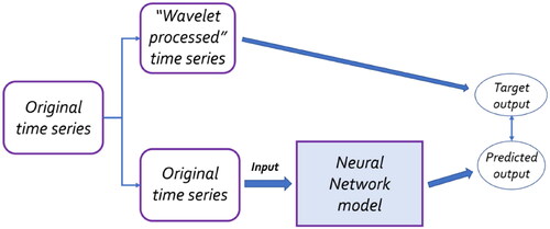
In the present study, we attempt to overcome these limitations by training a Neural Network (NN) to perform the equivalent of wavelet analysis on GNSS data. The main advantage is that a NN model, once trained, provides answers within seconds, thus making it feasible as a real-time data analysis tool. The proposed approach can be summarized as follows (Figure 1): i) the wavelet analysis is performed on GNSS time series from different stations in a permanent network; ii) a Convolutional Neural Network is trained using original time series as input and the ‘Wavelet processed’ series as target output; iii) the trained model is used on newly recorded GNSS data to perform real-time wavelet denoising.

Figure 1. Simplified flowchart of the proposed approach. The original signal is used as input, while its decomposed wavelet version is the target output.

2.1. Wavelet denoising

In the same way as the better-known Fourier transform, the wavelet transform measures the similarity between a signal and an analysing function. Both transforms use a mathematical tool called an inner product as a measure of similarity. The two transforms differ in the choice of analysing function. This results in different ways for the two transforms to represent the signal and the type of information that can be extracted. The wavelet concept was first introduced by Morlet (1983), then Grossmann and Morlet (1984) formalized the continuous wavelet transform (CWT), calculated as the inner product of the empirical wavelet function and the measured data $〈f,{\psi }_{a,b}〉,$ as follows: (1) $$W_{\psi }f\left(a,\mathrm{ }b\right)=〈f,{\psi }_{a,\mathrm{b}}〉=a^{-1/2}{\int }_{-\mathrm{\infty }}^{+\mathrm{\infty }}f\left(t\right)\overline{\psi }\left(\frac{t-b}{a}\right)dt,\mathrm{ }$$(1) where a indicates the scale parameter, b refers to the time parameter, ψ(t) is an analysing wavelet, and $\overline{\psi }$ symbolizes the complex conjugate of ψ. The inverse transform of CWT is given by (2) $$f\left(t\right)=\frac{1}{C_{\psi }}{\int }_{-\mathrm{\infty }}^{+\mathrm{\infty }}\left\{W_{\psi }f\left(a,\mathrm{ }b\right)\left[a^{-1/2}\psi \left(\frac{t-b}{a}\right)db\right]\right\}\frac{da}{a^2},\mathrm{ }$$(2) where a, b and t are continuous variables; therefore, they must be discretized in digital signal time series analysis. The discrete wavelet transform (DWT) derives from the discretization of the scale a and the time b, as in the following (3) $$a=a_0^j,\mathrm{ }b=k{a}_0^j{b}_0$$(3) with j and k as integers, so that the continuous wavelet function Wψf(a, b) transforms into the DWT, given by (4) $$C_{j,k}={\int }_{-\mathrm{\infty }}^{+\mathrm{\infty }}f\left(t\right){\overline{\psi }}_{j,k}\left(t\right)dt,\mathrm{ }$$(4) where, ψ_j,k(t)=2^-j/2(2^-jt-k). The inverse transform of DWT is defined by (5) $$f\left(t\right)=\sum _{j\in Z}\sum _{k\in Z}{C}_{j,k}{\psi }_{j,k}\left(t\right).\mathrm{ }$$(5)

Mallat (1989) proposed a fast DWT algorithm which decomposes and reconstructs the signal using the wavelet filters (Figure 2). The decomposition algorithm is given by (6) $$\left.\begin{array}{c}{A}_0\left[f\left(t\right)\right]=f\left(t\right)\\ A_j\left[f\left(t\right)\right]=\sum _{k}H\left(2t-k\right)A_{j-1}\left[f\left(t\right)\right]\\ D_j\left[f\left(t\right)\right]=\sum _{k}G\left(2t-k\right)A_{j-1}\left[f\left(t\right)\right]\end{array}\right\},\mathrm{ }$$(6) where t = 1, 2 …, N is the discrete time serial number, N is the signal length, f(t) represents the original signal, j = 1, 2 …, J is the decomposition level, J is the maximum decomposition level; H and G are the wavelet low-frequency and high-frequency pass decomposition filters, respectively, Aj and Dj are the wavelet coefficients of f(t) in the low-frequency and the high-frequency part of the j^th layer, respectively. The full set of H and G represents a filter bank that can use different scales; ten wavelet bandpass filters per octave are routinely used. The highest-frequency passband is designed so that the magnitude falls to half the peak value at the Nyquist frequency. Figure 2(a) shows the wavelet decomposition filter model.

Figure 2. Conceptual scheme of wavelet decomposition (a) and reconstruction filter model (b).

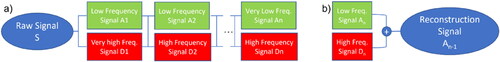
As a consequence of the wavelet filtering (Eq. (6)(6) $$\left.\begin{array}{c}{A}_0\left[f\left(t\right)\right]=f\left(t\right)\\ A_j\left[f\left(t\right)\right]=\sum _{k}H\left(2t-k\right)A_{j-1}\left[f\left(t\right)\right]\\ D_j\left[f\left(t\right)\right]=\sum _{k}G\left(2t-k\right)A_{j-1}\left[f\left(t\right)\right]\end{array}\right\},\mathrm{ }$$(6) ), each signal has the following decomposition and reconstruction relationship: S = A1 + D1; A1 = A2 + D2; A2 = A3 + D3; A3 = A4 + D4. In addition, the relationship of each signal is: S = a3 + d3 + d2 + d1, a3 = d3 + d2 + d1.

The reconstruction (Figure 2(b)) is given by (7) $$A_j\left[f\left(t\right)=\sum _{k}h\left(2t-k\right)A_{j+1}\left[f\left(t\right)\right]+\sum _{k}g\left(2t-k\right)D_{j+1}\left[f\left(t\right)\right]\right],\mathrm{ }$$(7) where h and g represent the wavelet low and high-pass reconstruction filter, respectively; other symbols are the same as in Eq. (6)(6) $$\left.\begin{array}{c}{A}_0\left[f\left(t\right)\right]=f\left(t\right)\\ A_j\left[f\left(t\right)\right]=\sum _{k}H\left(2t-k\right)A_{j-1}\left[f\left(t\right)\right]\\ D_j\left[f\left(t\right)\right]=\sum _{k}G\left(2t-k\right)A_{j-1}\left[f\left(t\right)\right]\end{array}\right\},\mathrm{ }$$(6) .

2.2. Convolutional neural networks

Originally developed for processing images, Convolutional Neural Networks (CNNs) are now successfully applied in different fields, ranging from speech recognition to self-driving cars (Borovykh et al. 2017; Gu et al. 2018). The main reason behind this success is the ability of CNNs to deal with spatial and temporal correlations, making them a powerful and effective tool in different contexts (Shin et al. 2016; Gu et al. 2018), which has proven to provide higher accuracy compared to other standard approaches (LeCun et al. 2015). This ability to handle temporal dependencies in the data prompted us to choose CNN over other Neural Network configurations. In fact, as stated in the previous section, the wavelet decomposition of a time series should better highlight temporal correlations in a time series by virtue of the increased signal-to-noise ratio and, consequently, emphasize the properties of the deformation field to be correlated with the field sources. Therefore, a NN sensitive to such correlations is crucial to achieve the highest possible accuracy in approximating the wavelet transform, which is the end goal of the present study.

A CNN is a multi-layered feed-forward neural network whose hidden layers are convolutional layers. The latter consist of different filters, which can be one or two-dimensional arrays of weights, depending on the input dimensions, and whose value is iteratively adjusted to improve the network accuracy. Specifically, each filter is moved over the input, performing a matrix multiplication each time until the complete input is covered. The final output of a convolutional layer with n filters consists of n filtered (or convolved) data. As the training goes on, the weights of the filters are automatically changed through a gradient descent algorithm and, by the end of the training process, each of these filters has learnt to extract different features from the same data. Once filtered, the data are usually sent to a downsampling layer, also known as a ‘pooling’ layer, which averages the filtered data. This process can be repeated an arbitrary number of times before sending the data to a final activation layer, to produce the expected output (e.g. an image label, a score, or a series of numbers).

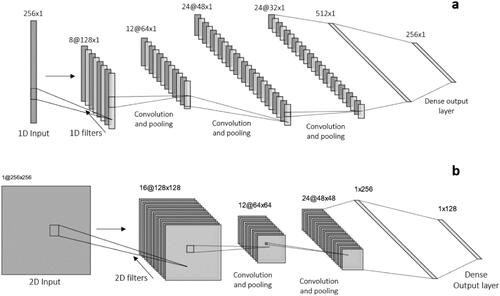
According to the filters’ dimension, a CNN can be 1D or 2D. Simplified examples of 1D and 2D CNN are shown in Figure 3. Further details on CNNs can be found in O’Shea and Nash (2015).

Figure 3. Examples of 1D and 2D Convolutional Neural Networks. (a) 1D input is filtered 8 times, producing, after a pooling layer, 8 filtered arrays with 128 x 1 elements; (b) 2D input is filtered 16 times, producing, after a pooling layer, 16 filtered images: each with 128 x 128 elements. In both configurations, the processing continues until a dense output layer is used to produce the desired output.

2.3. CNN as a ‘proxy’ wavelet

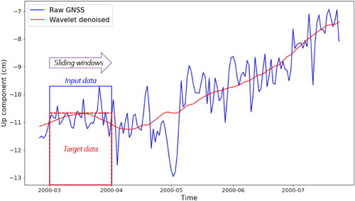
In the present research, a 1D Convolutional Neural Network is used to learn how to transform a noisy GNSS time series into a wavelet processed one. Thus, the input data is a time-window of GNSS time series and the target data is the same data window after wavelet denoising processing. The CNN is, therefore, trained to learn a non-linear transfer function between noisy time series and wavelet processed data by fine-tuning the filters’ weights and biases. An example of input and output is shown in Figure 4, where a GNSS (Up component) time series is used. It can be seen that input and output data are generated by moving a sliding time-window over a GNSS time series.

Figure 4. Input and target data for a GNSS time series. The input is a raw GNSS time series, while the target is its denoised wavelet. In this example, a 30-day window is used to train the data.

3. Application to the test area

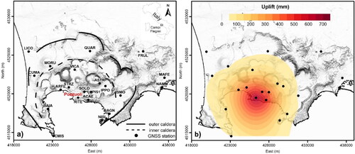
The proposed methodology was tested on daily GNSS vertical time series recorded in the Campi Flegrei volcanic area (Naples, Italy). This is a restless caldera, characterized by the bradyseism phenomenon, with repeated uplift episodes followed by subsidence periods. Several significant uplift episodes occurred in the last 100 years (namely the bradyseismic crises of 1950–1952, 1969–1972, and 1982–1984), with a total vertical displacement of about 4.3 m in Pozzuoli (Del Gaudio et al. 2010) (Figure 5). Since 2005, a new uplift phase has been observed and is still ongoing, with different rates over time (De Martino et al. 2021). The resulting total uplift recorded at the RITE GNSS station located in Pozzuoli is about 1 m. The ground deformation pattern, captured by GNSS data, shows a high degree of symmetry (bell-shaped geometry (Figure 5(b))), with a central sector where the RITE, ACAE and SOLO GNSS stations are located (Figure 5(a)), and where the maximum vertical displacements are observed, which decrease as one moves away from the caldera centre. The uplift phases are generally characterized by increased seismicity and high degassing activity; this is also the case at present (Chiodini et al. 2012, 2016; Giudicepietro et al. 2021; Tramelli et al. 2021, 2022). For this reason, the Campi Flegrei volcanic area is a suitable site to test our algorithm, as the availability of reliable GNSS data in this context is of crucial importance for both volcano monitoring and hazard assessment (Rosi et al. 2022).

Figure 5. (a) Schematic map of Campi Flegrei caldera with location of GNSS stations; (b) vertical deformation pattern from 2016 to 2022.

3.1. Dataset and pre-processing

The dataset used in this research consisted of daily GNSS time series (De Martino et al. 2021) recorded by the Neapolitan Volcanoes Continuous GPS (NeVoCGPS) network, operated by the Istituto Nazionale di Geofisica e Vulcanologia–Osservatorio Vesuviano (INGV-OV), developed in the early 2000s for ground deformation monitoring of the Campi Flegrei caldera, Somma–Vesuvius volcano, and Ischia–Procida Islands. Currently, the network comprises 37 permanent stations and 21 of them are operating in the Campi Flegrei area (see Figure 5(a)). For further details on the NeVoCGPS network design, instrumentation, data management and data processing, the reader is referred to De Martino et al. (2021).

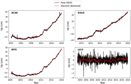
The Campi Flegrei daily GNSS vertical displacement represents the input dataset. Since the ground deformation in the Campi Flegrei caldera consists mostly of vertical movements, we chose to focus only on the Up component of each GNSS station. The output dataset is the wavelet decomposition of the original time series. The maximal overlap discrete wavelet transform (MODWT) function implemented in Matlab® was used to obtain a low-pass filtered component of the time series. Two important steps characterize the wavelet denoising: i) the choice of the appropriate wavelet function Wψf(a, b); and ii) the selection of the decomposition level. Regarding the choice of the wavelet function, the Daubechies (dbN) and Haar and Symlets (SymN) functions are commonly used for wavelet analysis. Since the main goal of this step of the proposed methodology was to obtain a smoother signal to be used for training a Convolutional Neural Network, we did not carry out a detailed study to produce the best possible wavelet denoising result. However, several authors (Chen et al. 2019) have shown that when the decomposition level is less than 6, the three mentioned wavelets produce very similar performance. Concerning the choice of decomposition level, since our aim was to increase the signal-to-noise ratio, we had to choose which signal was useful. In order to target the test method in an area of geodynamic relevance, due to bradyseism (i.e. slow ground uplift), which was expected to detect a trend in the daily GNSS time series, we arbitrarily set a spectral limit between the useful signals and noise to clean up the trend. We considered the low frequency component (f < 0.03 cycles/day; T > ∼30 days) of the raw signal as the useful signal and then designed a 'low-pass’ wavelet reconstruction filtering with a suitable cut-off frequency. We decided not to set a ‘severe’ cut-off frequency, to preserve near-monthly oscillations that have been highlighted by several authors (Romano et al. 2018; Tammaro et al. 2021) in the Campi Flegrei ground deformation. Therefore, frequencies greater than 0.03 cycles/day were suitably eliminated by settling the wavelet development at level 5. As an example, Figure 6 shows the results of wavelet decomposition under Sym4 wavelet with decomposition level 5, and the original signal S is the GNSS time series collected at the RITE station of the NeVoCGPS network (see Figure 5). The following only considers the results provided by the Sym4 wavelet with decomposition level 5, for a subset of four selected GNSS stations, three of which are in the central sector of the Campi Flegrei caldera (ACAE, SOLO, RITE in Figure 7), currently characterized by the most intense dynamics. The fourth (LICO in Figure 7) is located outside the caldera and reflects a different level of deformation than the previous three stations.

Figure 6. Results of wavelet decomposition of Sym4 wavelet at level 5 (S = a5 + d5 + d4 + d3 + d2 + d1).

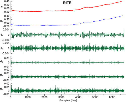
Figure 7. GNSS vertical daily time series collected at four selected permanent stations in the Campi Flegrei area (see Figure 5 to locate the stations).

3.2. Network structure and hyperparameter tuning performance evaluation

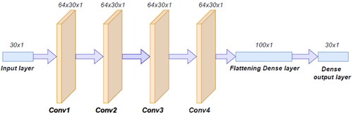
As described in Section 2.2, a Convolutional Neural Network (CNN) consists of layers of filters. The number of layers and filters per layer must be chosen in advance, before starting the training process. The optimal number of both cannot be determined theoretically; however, as a rule of thumb, we followed the Occam’s razor approach and selected the simplest possible configuration from those which provided the highest accuracy. Thus, the selection of the final CNN followed a trial and error phase, where different configurations were tested. This network consists of four convolutional layers, each with 64 filters and a kernel of size 3 (Figure 8). The last layer is a flattening layer that receives the filtered time series and transforms them into a 1D vector. Once defined, the network architecture and optimization hyperparameters were selected. We tested different configurations and achieved the highest accuracy with the Adam optimizer and the mean absolute error loss function.

Figure 8. Schematic structure of the CNN used in this work. The initial time-window input is passed through four convolutional layers with 64 filters before reaching the final output layers.

An additional parameter that must be defined before starting the training is the length of the GNSS time series window. We chose to focus on 30-day time-windows because, as mentioned before, they may include significant deformation patterns. However, we also applied our methodology to different time-window lengths and the obtained results are shown in Section 4.

3.3. Performance evaluation

To assess the accuracy of the developed model, we used two metrics: Root Mean Square Error (RMSE) and coefficient of determination (R²). These are standard metrics, commonly employed with time series modelling and regression problems (Brockwell and Davis 2016). Specifically, the RMSE is the square root of the average of the square of all the errors: (8) $$\mathit{RMSE}=\mathrm{ }\sqrt{\frac{1}{n}\sum _{t=1}^n{(S_t-O_t)}^2},\mathrm{ }$$(8) where S_t and O_t are the predicted and observed values of the target variable, respectively. The RMSE is measured in the same units as the predicted quantity, which makes it possible to quantify the average distance of each prediction from the true value. On the other hand, the coefficient of determination, R², quantifies the amount of variance of the observed data that is explained by the developed model. It is, therefore, a measure of the quality of the fit and is estimated as follows: (9) $$R^2=1-\mathrm{ }\frac{\sum _{t=1}^n{\left(S_t-O_t\right)}^2}{\sum _{t=1}^n{\left(S_t-\overline{O}\right)}^2},\mathrm{ }$$(9) where $\overline{O}$ represents the average of the observations. R² can theoretically vary between -$\mathrm{\infty }$ and 1; however, it is usually confined between 0 and 1. A value close to 0 implies that the model perfectly predicts the average value of the observed data, while a value close to 1 means that the model perfectly predicts the observed values.

Like all metrics, both the RMSE and the R² score have some limitations. Indeed, the RMSE does not consider the magnitude of the observed values and, therefore, does not provide information about the relative or percentage error in the estimates, which is sometimes as important as the average distance. On the other hand, R² is heavily influenced by the outliers as it is a squared measure. The presence of a single outlier in a set of otherwise good predictions can severely decrease R², erroneously leading to the discarding of a model. Only the combination of both the metrics, aided by visual evaluation of the predictions, allows us to have a clear picture of the model’s accuracy.

4. Results

The proposed methodology was tested on data coming from all of the 21 stations in the NeVoCGPS monitoring network. However, for the sake of brevity, only the results obtained for the four stations in Figure 7 (RITE, ACAE, SOLO and LICO) are shown.

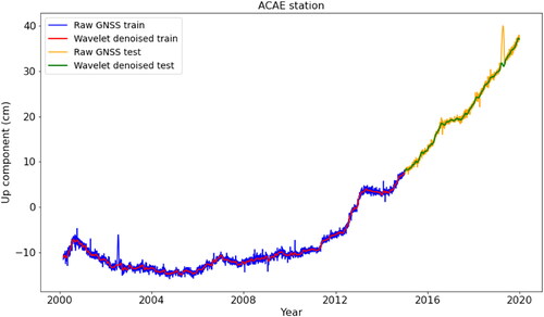
For each time series, the dataset was split into a ‘training’ and a ‘test’ set, with a ratio of 75:25, namely the first 75% of the data was used for training and the remaining 25% for testing, as shown in Figure 9. The latter presents an example of the training and test sets used for the ACAE station.

Figure 9. Example of training and test sets for both the input (train and test data in the legend) and the output (denoised wavelet in the legend).

The quality of the predictions obtained for the four selected stations is high overall (Figure 10 and Table 1), with a minimum R² value of 0.72 for the LICO station and a maximum of 0.98 for both the SOLO and RITE stations. The RMSE also reflects a high accuracy, with a minimum value of 0.22 cm for the SOLO station and a maximum value of 1.16 cm for the ACAE station. It is worth noting that when a deformation trend is present in the time series, the quality of the predictions seems to decrease slightly with time. This can be explained by the train-test split used to develop the model. In fact, the model was tested on the last 25% of the data. Therefore, by moving forward in time, the distance from the last training data window increases and, thus, there is the possibility that new ‘undetected’ trends or noise will appear in the data. If new trends and/or noise affect the data, even if they are small, the network may fail to predict them, as it has never trained on them, and this could result in a slight decrease of the prediction accuracy. Such an occurrence is a consequence of the well-known behaviour of time series, which tend to show a stronger temporal correlation with recent data than with data further back in time. However, it should be noted that this will not be a problem in real-time applications, since the developed network will be constantly retrained once new data are acquired.

Figure 10. Prediction results obtained on test data for ACAE, SOLO, RITE and LICO stations.

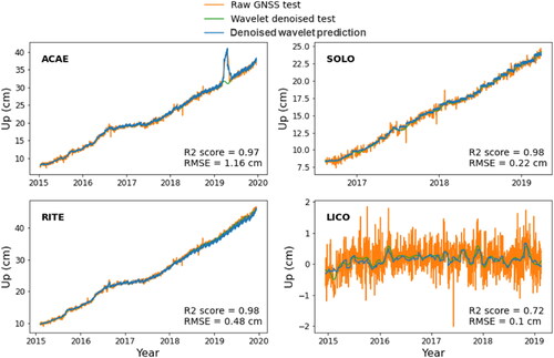
Table 1. Accuracy metrics resulting from 30-day window test sets for each station of the Campi Flegrei section of the NeVoCGPS network.

Station	R^2	RMSE (cm)
ACAE	0.97	1.16
ARFE	0.98	0.32
ASTR	0.94	0.15
BAGN	0.93	0.16
BAIA	0.98	0.25
CMIS	0.75	0.11
CUMA	0.53	0.14
FRUL	0.13	0.36
IPPO	0.97	0.24
ISMO	0.39	0.2
LICO	0.65	0.11
MORU	−5.02	1.91
NISI	0.96	0.29
PIS1	0.97	0.25
QUAR	0.97	0.33
SOLO	0.98	0.22
VICA	0.97	0.02
RITE	0.98	0.48

Table 1 lists the prediction accuracy for 18 stations of the NeVoCGPS monitoring network in the Campi Flegrei caldera, the prediction accuracy being high overall. In fact, the prediction quality is only low for three stations, i.e. FRUL, IPPO and MORU, with a negative R² score for the last two stations. A further analysis of the GNSS time series for these three stations suggests that the obtained low-quality predictions are likely to be related to the presence of large gaps in the training data, probably due to temporary station malfunctions. When a CNN model is trained only on the portion of these signals without gaps, a high accuracy is also obtained for these three stations. These results show that the proposed methodology can only be successfully applied to continuous GNSS time series, or whenever only small gaps (1–2 days) affect the recordings, which can be effectively treated with interpolation techniques. In the case of longer (>2 days) data gaps, indeed, the data retrieved with any interpolation technique are not reliable and, consequently, the Wavelet decomposition fails. When such a bias is introduced in the input data, the NN learning capability is severely limited.

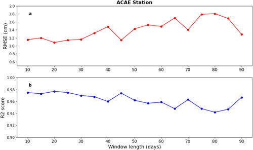
The effect of the time-window length was analysed by applying the proposed methodology to different time-windows. Figure 11 shows the results obtained for the ACAE GNSS station and it can be seen that the variability of RMSE and R² as a function of the window length indicates that the accuracy remains high with a time-window length ranging from 10 to 90 days. This result is promising, as it suggests that the developed denoising technique is robust and can be successfully used to process even shorter time windows, which can be useful for real-time applications.

Figure 11. RMSE (a) and R² (b) as a function of window length for the ACAE station.

5. Conclusions

In this study, we propose a new GNSS data denoising strategy for recognizing transients in ground deformation time series that could be used in real-time as a monitoring tool for active volcanic and geodynamic areas. It is well known that such areas can show very rapid changes in physical parameters and the early recognition of such variations can be crucial in recognizing the precursors of imminent phenomena, such as eruptive activity, alluvial plain subsidence, etc. We have, therefore, aimed to develop a technique based on Machine Learning with a high degree of computational efficiency, which is capable of outperforming classical denoising techniques. Specifically, the proposed strategy aims to denoise GNSS data by training a Convolutional Neural Network to perform an equivalent of the wavelet decomposition on such data. In this way, the power of the wavelet denoising could also be exploited in those situations where a real-time analysis is required.

The developed methodology has been tested on GNSS time series data recorded at the Campi Flegrei volcanic area, which is characterized by intense uplift periods followed by subsidence phases (bradyseism). The effectiveness of the proposed approach is testified by the RMSE and R² values obtained for the 21 analysed GNSS stations, which reflect an overall high accuracy of the retrieved predictions, as well as the robustness of the developed denoising technique in processing even short time windows of the GNSS data sets. In particular, it should be noted that, when the time series do not present huge recording gaps, the RMSE and R² values vary in the ranges 0.65-0.98 and 0.06-0.52 cm, respectively. These findings are promising, as they suggest that the proposed methodology can be successfully applied for the GNSS data denoising, paving the way for the development of more effective real-time monitoring solutions.

Acknowledgements

The authors are grateful to the Associated Editor and two anonymous Reviewers for their comments and suggestions that improved the paper.

Disclosure statement

No potential conflict of interest was reported by the author(s).

Data availability statement

The data that support the findings of this study are available from the corresponding author [UR] upon reasonable request.

References

- Amos CB, Audet P, Hammond WC, Bürgmann R, Johanson IA, Blewitt G. 2014. Uplift and seismicity driven by groundwater depletion in central California. Nature. 509(7501):483–486.
- Argus DF, Heflin MB, Peltzer G, Crampé F, Webb FH. 2005. Interseismic strain accumulation and anthropogenic motion in metropolitan Los Angeles. J Geophys Res. 110: b04401.
- Bai L, Han Z, Li Y, Ning S. 2018. A hybrid denoising algorithm for the gear transmission system based on CEEMDAN-PE-TFPF. Entropy. 20(5):361.
- Bock Y, Melgar D. 2016. Physical applications of GPS geodesy: a review. Rep Prog Phys. 79(10):106801.
- Borovykh A, Bohte S, Oosterlee CW. 2017. Conditional time series forecasting with convolutional neural networks. ArXiv. https://doi.org/10.48550/arxiv.1703.04691.
- Borsa AA, Agnew DC, Cayan DR. 2014. Remote hydrology. Ongoing drought-induced uplift in the western United States. Science. 345(6204):1587–1590.
- Brockwell PJ, Davis RA. 2016. Introduction to time series and forecasting. Cham: Switzerland AG Springer.
- Chen Z, Liu B, Yan X, Yang H. 2019. An improved signal processing approach based on analysis mode decomposition and empirical mode decomposition. Energies. 12(16):3077.
- Chiodini G, Caliro S, De Martino P, Avino R, Gherardi F. 2012. Early signals of new volcanic unrest at Campi Flegrei caldera? Insights from geochemical data and physical simulations. Geology. 40(10):943–946.
- Chiodini G, Paonita A, Aiuppa A, Costa A, Calir S, De Martino P, Acocella V, Vandemeulebrouck J. 2016. Magmas near the critical degassing pressure drive volcanic unrest towards a critical state. Nat Commun. 7:13712.
- Cui B, Chen X. 2015. Improved hybrid filter for fiber optic gyroscope signal denoising based on EMD and forward linear prediction. Sensors Actuat A: Phys. 2(30):150–155.
- De Martino P, Dolce M, Brandi G, Scarpato G, Tammaro U. 2021. The ground deformation history of the Neapolitan volcanic area (Campi Flegrei Caldera, Somma–Vesuvius Volcano, and Ischia Island) from 20 years of continuous GPS observations (2000–2019). Remote Sens. 13(14):2725.
- Del Gaudio C, Aquino I, Ricciardi GP, Ricco C, Scandone R. 2010. Unrest episodes at Campi Flegrei: a reconstruction of vertical ground movements during 1905–2009. J Volcanol Geoth Res. 195(1):48–56.
- Devoti R, De Martino P, Pietrantonio G, Dolce M. 2018. Coseismic displacements on Ischia island, real-time GPS positioning constraints on earthquake source location. Ann Geophys. 61(3):SE337.
- Dong D, Fang P, Bock Y, Webb F, Prawirodirdjo L, Kedar S, Jamason P. 2006. Spatiotemporal filtering using principal component analysis and Karhunen-Loeve expansion approaches for regional GPS network analysis. J Geophys Res. 111: b03405.
- Giudicepietro F, Ricciolino P, Bianco F, Caliro S, Cubellis E, D’Auria L, De Cesare W, De Martino P, Esposito AM, Galluzzo D, et al. 2021. Campi Flegrei, Vesuvius and Ischia Seismicity in the Context of the Neapolitan Volcanic Area. Front Earth Sci. 9:662113.
- Grinsted A, Moore JC, Jevrejeva S. 2004. Application of the cross wavelet transform and wavelet coherence to geophysical time series. Nonlin Processes Geophys. 11:561–566.
- Grossmann A, Morlet J. 1984. Decomposition of hardy functions into square integrable wavelets of constant shape. SIAM J Math Anal. 15(4):723–736.
- Gu J, Wang Z, Kuen J, Ma L, Shahroudy A, Shuai B, et al. 2018. Recent advances in convolutional neural networks. Pattern Recognit. 77:354–377.
- He X, Hua X, Yu K, Xuan W, Lu T, Zhang W, Chen X. 2015. Accuracy enhancement of GPS time series using principal component analysis and block spatial filtering. Adv Space Res. 55:1316–1327.
- He X, Montillet J-P, Fernandes R, Bos M, Yu K, Hua X, Jiang W. 2017. Review of current GPS methodologies for producing accurate time series and their error sources. J Geodyn. 106:12–29.
- Huang NE, Shen Z, Long SR, Wu MC, Shih HH, Zheng Q, Yen N-C, Tung CC, Liu HH. 1998. The empirical mode decomposition and the Hilbert spectrum for non-linear and non-stationary time series analysis. Proc Royal Soc London A Math Phys Eng Sci. 454(1971):903–995.
- King NE, Argus D, Langbein J, Agnew DC, Bawden G, Dollar RS, Liu Z, Galloway D, Reichard E, Yong A, et al. 2007. Space geodetic observation of expansion of the San Gabriel Valley, California, aquifer system, during heavy rainfall in winter 2004–2005. J Geophys Res. 112(B3):B03409.
- Larson KM, Poland M, Miklius A. 2010. Volcano monitoring using GPS: developing data analysis strategies based on the June 2007 Kīlauea Volcano intrusion and eruption. J Geophys Res. 115(B7):B07406.
- LeCun Y, Bengio Y, Hinton G. 2015. Deep learning. Nature. 521(7553):436–444.
- Li W, Shen Y. 2018. The consideration of formal errors in spatiotemporal filtering using principal component analysis for regional GNSS position time series. Remote Sensing. 10:534.
- Mallat SG. 1989. A theory for multiresolution signal decomposition: the wavelet representation. IEEE Trans Pattern Anal Mach Intell. 11(7):674–693.
- Milliner C, Materna K, Bürgmann R, Fu Y, Moore AW, Bekaert D, Adhikari S, Argus DF. 2018. Tracking the weight of Hurricane Harvey’s stormwater using GPS data. Scientific Adv. 4(9):eaau2477.
- Morlet J. 1983. Sampling theory and wave propagation. Issues in acoustic signal—image processing and recognition. Nato Asi. 1:233–261.
- O'Shea K, Nash R. 2015. An introduction to convolutional neural networks. ArXiv:1511.08458 [Cs]. http://arxiv.org/abs/1511.08458
- Riccardi U, Arnoso J, Benavent M, Velez E, Tammaro U, Montesinos FG. 2018. Exploring deformation scenarios in Timanfaya volcanic area (Lanzarote, Canary Islands) from GNSS and ground based geodetic observations. J Volcanol Geotherm Res. 357:14–24.
- Romano V, Tammaro U, Riccardi U, Capuano P. 2018. Non-isothermal momentum transfer and ground displacements rate at Campi Flegrei caldera (Southern Italy). Phys Earth Planet Inter. 283:131–139.
- Rosi M, Acocella V, Cioni R, Bianco F, Costa A, De Martino P, Giordano G, Inguaggiato S. 2022. Defining the pre-eruptive states of active volcanoes for improving eruption forecasting. Front Earth Sci. 0:170.
- Serpelloni E, Faccenna C, Spada G, Dong D, Williams SDP. 2013. Vertical GPS ground motion rates in the Euro-Mediterranean region: new evidence of velocity gradients at different spatial scales along the Nubia-Eurasia plate boundary. J Geophys Res Solid Earth. 118(11):6003–6024.
- Shin HC, Roth HR, Gao M, Lu L, Xu Z, Nogues I, Yao J, Mollura D, Summers RM. 2016. Deep convolutional neural networks for computer-aided detection: CNN architectures, dataset characteristics and transfer learning. IEEE Trans Med Imaging. 35(5):1285–1298.
- Tammaro U, Obrizzo F, Riccardi U, La Rocca A, Pinto S, Brandi G, Vertechi E, Capuano P. 2021. Neapolitan volcanic area Tide Gauge Network (Southern Italy): ground displacements and sea-level oscillations. Adv Geosci. 52:105–118.
- Tao Y, Liu C, Liu C, Zhao X, Hu H. 2021. Empirical wavelet transform method for GNSS coordinate series denoising. J Geovis Spat Anal. 5:9.
- Tian Y, Shen Z-K. 2016. Extracting the regional common-mode component of GPS station position time series from dense continuous network. J Geophys Res Solid Earth. 121:1080–1096.
- Tramelli A, Giudicepietro F, Ricciolino P, et al. 2022. The seismicity of Campi Flegrei in the contest of an evolving long term unrest. Scientific Rep. 12:2900.
- Tramelli A, Godano C, Ricciolino P, Giudicepietro F, Caliro S, Orazi M, et al. 2021. Statistics of seismicity to investigate the Campi Flegrei Caldera unrest. Scientific Rep. 11:7211.
- Tregoning P, van Dam T. 2005. Atmospheric pressure loading corrections applied to GPS data at the observation level. Geophys Res Lett. 32(22):L22310.
- Vitagliano E, Riccardi U, Piegari E, Boy J-P, Di Maio R. 2020. Multi-component and multi-source approach for studying land subsidence in deltas. Remote Sens. 12(9):1465.
- Wdowinski S, Bock Y, Zhang J, Fang P, Genrich J. 1997. Southern california permanent GPS geodetic array: spatial filtering of daily positions for estimating coseismic and postseismic displacements induced by the 1992 Landers earthquake. J Geophys Res. 102(B8):18057–18070.