A local regression approach to analyze the orographic effect on the spatial variability of sub-daily rainfall annual maxima

Abstract

In this work we investigate the spatial variability of sub-daily rainfall extremes over Italy considering the influence of local orographic effects. We consider the average annual maxima computed from the recently-released Improved Italian – Rainfall Extreme Dataset (I²-RED) in about 3800 time series with at least 10 years of data (1916–2020 period) and we analyze the orographic effects through a local regression approach which gathers stations in a grid cell-centered area of 1 km resolution. Several constraints are considered to tackle problems determined by the low data density of some areas and by the extrapolation at low/high elevations. Different criteria for selecting the local sample are examined. This work confirms with increased detail previous findings, such as a generally positive gradient of the 24 h average annual maxima and the evidence of negative gradients in large mountainous areas for the 1 h maxima. The use of a local regression approach allows to identify the areas showing the reverse orographic effect, providing material for future investigations on the physical explanation of this evidence. Moreover, the reconstructed maps will allow to apply more accurate approaches in works related to the spatial variability of other rainfall statistics, such as the quantiles required for hydrologic design.

Keywords:

• Rainfall
• extremes
• elevation
• orographic effect
• Italy

1. Introduction

Datasets of rainfall features with large coverage in space and time can be relevant in a vast range of applications, like hydraulic design, water resources management and climate change impact assessment. Not many of these datasets refer to the features of precipitation extremes, which are of increasing interest for both scientists and practitioners because of the evolution of the hydrologic hazard in the recent years (Fowler et al. 2021a, 2021b).

Dataset related to large areas are generally created by spatial interpolation of irregularly spaced rain gauge data into a regular grid (Daly et al. 1994, 2002; Thornton et al. 2021; Crespi et al. 2018). To control the quality of the interpolation it is necessary to understand the spatial distribution of the rainfall features, particularly by investigating some geographic factors that can be considered responsible for the spatial variability of the rainfall amounts. One such factor is the relief.

In regions with almost flat orography, rainfall variability can be handled with interpolation techniques (e.g. inverse distance weighting and ordinary kriging) that do not require to consider other spatial covariates. On the other hand, in regions with significant elevation variability, interpolation requires methods that can explicitly account for the elevation effect (e.g. Prudhomme and Reed 1999; Daly 2006; Claps et al. 2022). Several of the approaches available in the literature consider the elevation as an explanatory variable, such as: simple and multiple regression models (Basist et al. 1994; Prudhomme and Reed 1998, 1999; Allamano et al. 2009; Mazzoglio et al. 2022), local regressions or georegressions (Daly et al. 1994), geographically-weighted regressions (Thornton et al. 1997; Brunsdon et al. 2001; Daly et al. 2002; Di Piazza et al. 2011; Crespi et al. 2018; Thornton et al. 2021), residual or regression kriging (Prudhomme and Reed 1999; Di Piazza et al. 2011; Crespi et al. 2018), kriging with external drift (Goovaerts 1999; Pellicone et al. 2018) and cokriging (Diodato and Ceccarelli 2005; Pellicone et al. 2018).

Among the methods listed above, univariate and multivariate linear regression models have the advantage of producing results that are statistically stable with respect to small errors in the observations; they also explain a large portion of the rainfall variability (Daly 2006). Nevertheless, when applied to large areas with complex terrain features, the use of a unique regression model can lead to evident clustering of the residuals. This is why simple or multiple linear regressions usually provide better results if applied over small regions (Daly 2006; Mazzoglio et al. 2022).

Geographically-weighted regression techniques have been developed to deal with local relationships between rainfall and geography. For instance, in the first version of PRISM, i.e. the Parameter-elevation Regressions on Independent Slopes Model (Daly et al. 1994), the precipitation-elevation relationship is investigated with reference to any individual grid cell. The approach uses a local regression model that selects rain gauges located within a specific radius on topographic facets having an orientation similar to the one of the estimation cell. An improved version of PRISM (Daly et al. 2002) uses a complex geographically-weighted regression model based on weighting functions that account, for every station, for the effects of elevation, terrain orientation, coastal proximity and a two-layer atmosphere introduced to handle non-monotonic variations with the elevation (Daly et al. 2002; Daly 2006). In both the PRISM versions, the optimal search radius is identified through cross-validation and ranges from 30 to 100 km, in an attempt to adapt to the station density. Other works (Brunsdon et al. 2001; Fotheringham et al. 2002) implemented a geographically-weighted regression with fixed or adaptive spatial kernels (using a Gaussian or exponential decay function). These latter approaches avoid the a priori selection of the radius used to select the points in the analysis of the spatially varying precipitation vs elevation relationships. A mixed approach is used in the Daymet model (Thornton et al. 1997, 2021): a truncated Gaussian spatial kernel is applied only to stations located within a specific search radius defined using a data density evaluation algorithm. In all these applications, each rain gauge included in the regression function is weighted by its distance from the grid cell where rainfall is to be estimated. This approach makes data measured far from the target cell irrelevant.

Due to the lack of a complete national rainfall database, until recently, analyses based on geo-regression models were not extensively conducted over Italy. The only study available for the entire country (Crespi et al. 2018) considers monthly and annual precipitations. Some studies are available for selected regions of Italy: Di Piazza et al. (2011) focused on monthly rainfall in Sicily, Golzio et al. (2018) and Crespi et al. (2021) analyzed monthly rainfall in the Central Alps region, while Frei and Schär (1998) and Isotta et al. (2014) addressed daily rainfall in Northern Italy. None of them, whatever the spatial coverage, has considered rainfall extremes of sub-daily durations.

In addressing the goal of accurately reconstructing sub-daily extreme rainfall indices (as the mean values, that is the focus of this work) at a national scale, we can take advantage of: i) a database of sub-daily annual maximum rainfall depths (Mazzoglio et al. 2020) and ii) some preliminary results reported in Mazzoglio et al. (2022) that demonstrated the influence of elevation in the spatial variability of sub-daily annual maxima. Within the framework of the spatial analysis of rainfall extremes, and based on the above considerations, the aims of this research are to: i) investigate the relationships between orography and the mean values of the sub-daily annual maximum rainfall depths (the so-called ‘index rainfall’ (Dalrymple 1960)) in Italy and ii) build maps of sub-daily average annual maxima that can be used for describing the spatial variability of the extremes over Italy. Both these issues represent the main novelties introduced in this work, in which we develop: i) a new criteria for the definition of the optimal search radius on the basis of the station density, as an extension of something attempted in Daymet (Thornton et al. 2021); ii) a methodology that allows to investigate the presence of negative orographic gradients for short durations (according to Allamano et al. 2009; Avanzi et al. 2015; Mazzoglio et al. 2022), not considered in PRISM; iii) an approach for the selection of constraints in the process of pooling the local sample, that can solve some well-known artifacts remarked in Daymet, such as negative or excessive estimated values; iv) new maps of sub-daily average annual maximum rainfall depths in Italy. The approach undertaken is based on an improved local regression approach, that is able to preserve local features and to prevent the spatial clustering of the residuals.

2. Methods

The nature of the approach proposed involve a strict relationship between data and methods. The reason is that the selection of the sample to be subjected to local regression is based itself on the quality of the results of the regression applied. In this section, the interactions between the two components is preliminary exposed.

2.1. Data catalog

Rainfall data used in this analysis comes from the Improved Italian – Rainfall Extreme Dataset (I²-RED; Mazzoglio et al. 2020), a collection of short-duration (1, 3, 6, 12 and 24 h) annual maximum rainfall depths measured from 1916 until 2020 by more than 5200 rain gauges located over Italy. In this study we use only time series with at least 10 years of data (from more than 3800 stations). At-site average annual maxima for the 5 durations are computed and constitute our reference data catalog.

In this work, we do not consider the possible variability of the mean values over time. Regarding the area of interest of this work, previous studies (Libertino et al. 2019; Mazzoglio et al. 2022) pointed out that an increase in rainfall extremes over the entire territory is not detectable and not statistically significant over a large part of Italy. Therefore, we decided to consolidate the knowledge in the perspective of stationarity.

Elevation data of the rain gauges and of the surrounding terrain come from the Shuttle Radar Topography Mission (STRM) Digital Elevation Model (DEM) at 30 m resolution (Farr et al. 2007) resampled at 1-km resolution using a cubic interpolation, as in Daymet (Thornton et al. 2021). The elevation of the rain gauges was derived from the resampled DEM using the station coordinates, following the approach suggested in PRISM (Daly et al. 1994, 2002) and adopted in Daymet (Thornton et al. 1997, 2021). This step is not trivial and has methodological implications. In fact, the authors involved in the development of PRISM pointed out that the relationship between precipitation and elevation is more representative if local elevations are derived from a low-resolution DEM, that is able to describe better the scale of orographic processes and to filter out local elevation details.

2.2. Linear regression model

In order to examine the relations between sub-daily rainfall depths and orography, local linear regression models have been built. The linear regression model that we use is (1) $$h_d=\mathit{\text{a}}+\mathit{\text{b}}\times \mathit{\text{z}}+\mathrm{\epsilon }$$(1) where h_d is the average annual maximum of an assigned duration d (with d = 1, 3, 6, 12 and 24 h in our case), a is the intercept, b is the slope (that represents the rainfall gradient), z is the elevation and ε is the residual of the regression.

As mentioned in the Introduction, approaches that use a unique linear regression model applied over vast areas are known to produce high residuals and high bias (see also Brunsdon et al. 2001; Mazzoglio et al. 2022). For this reason, we allow the parameters a and b to be space-dependent, i.e. Eq. (1)(1) $$h_d=\mathit{\text{a}}+\mathit{\text{b}}\times \mathit{\text{z}}+\mathrm{\epsilon }$$(1) assumes the form (2) $$h_d(x,y)=a(x,y)+b(x,y)\times z(x,y)+\mathrm{\epsilon }(x,y)$$(2) where h_d, a, b, z and ε have the same meaning as in Eq. (1)(1) $$h_d=\mathit{\text{a}}+\mathit{\text{b}}\times \mathit{\text{z}}+\mathrm{\epsilon }$$(1) but are related to a generic position with coordinates (x,y).

Similarly to the Daymet model (Thornton et al. 1997), we consider linear rainfall-elevation relationships by using slope coefficients b(x,y) dependent only on the planimetric coordinates. In most applications of the PRISM model, the minimum allowable slope coefficient b(x,y) is set to zero, because Daly et al. (2002) argue that the rainfall depth can only increase with elevation. Considering that previous works conducted over Italy suggest that a reduction of rainfall depth with elevation is possible (e.g. Allamano et al. 2009; Avanzi et al. 2015; Libertino et al. 2018; Formetta et al. 2022; Mazzoglio et al. 2022), in our work we do not disregard negative values obtained for the b(x,y) parameter. Nevertheless, values of the b(x,y) parameter need to be in a reasonable range, as will be explained in Section 3.3.

2.3. Local sample identification

To estimate the parameters of the local regression (Eq.2(2) $$h_d(x,y)=a(x,y)+b(x,y)\times z(x,y)+\mathrm{\epsilon }(x,y)$$(2) ) in every (x,y) position, a ‘local’ reference sample must be identified with a number n of station included in an area adequate for a regression. Similarly to Daly et al. (2002), we proceed by selecting n stations available in a circular area of radius r, whose center coincides with the centroid of the grid cell to which the regression is referred. The length of the radius and the minimum number of stations required for reaching a reasonable local estimate are parameters that have to be conveniently tuned.

If r is small, a low number of rain gauges would be selected (in some cases, the low data density can imply that no rain gauge can be selected). If r is large, the relationship ceases to be ‘local’, and model performance can degrade. The definition of the number of stations necessary for the regression is strongly driven by the station density and its uniformity on the territory, being desirable that the regression model is applicable on a high percentage of the territory. To provide a baseline, we started to use local samples gathered in circles of varying radii, to perform a rain gauge density analysis. The search of the modal value of stations available in circles of different radius can be a first approach for defining n. As a reference, when the PRISM model considers all the stations (independently on the orientation of the topographic facet on which these stations are installed), the authors account for the availability of 10 to 30 stations within a radius of 30 to 100 km (Daly et al. 2002).

To define the most appropriate radius of the area needed for selecting the local sample, in this work two approaches have been adopted:

• to use a unique, fixed radius r = r_fix;

• to use a radius interval, variable from r_min to r_max, that depends on data density.

In the first approach we evaluate the regression parameters using the data of rain gauges that are located inside a circular area of radius r = r_fix, whatever the statistical significance of the regression model. This approach is similar to the one used in the PRISM and in Daymet models. In the second approach, the radius increases from r_min to r_max in each cell, until a statistically-significant regression model is found (p-value < 0.05). The r_max is set to avoid regression models that gather data from areas that are too large. If, when reaching r_max, the model pools together at least n rain gauges, but the regression is not statistically significant, two alternatives can be considered: a) the model is applied without considering the p-value threshold; b) the predicted value is set to the mean rainfall value evaluated using the n nearest stations. If n stations are not present even within a circle of radius r_max, the model is applied to the n nearest stations, regardless of their position.

It is worthwhile to observe that the evaluation of the average annual maxima, using the mean values of the n nearest stations, can be applied all over the territory. This approach, despite its simplicity, can provide a valid starting point for additional comparisons with most complex methods. It is interesting to notice that all the previously referenced works do not provide this comparison.

2.4. Artifacts and model corrections in high/low elevations

Application of systematic criteria for the selection of both the local sample and of the reference radius can involve the presence of artifacts in the final results. The analyses carried out in this research have shown that artifacts are mainly due to two causes: i) a non-consistent rainfall gradient; and ii) a level of extrapolation leading to unreasonable results.

As regards the first issue, we realized that an insufficient elevation range in the data sample was the cause of anomalously high (positive and negative) rainfall local gradient. To prevent the occurrence of this effect, we envisaged to impose a minimum elevation range Δz (i.e. the difference between the highest and the lowest rain gauge) to undergo to the regression analysis.

Considering the extrapolation aspects, it is well known that regression models applied in data scarce regions with a complex rainfall-elevation relationship can produce unrealistic results (Brunsdon et al. 2001; Crespi et al. 2018). In Crespi et al. (2018) no constraint is assigned to grid cells with elevation higher than those of the rain gauges used in the local sample. Also in the first version of PRISM model (Daly et al. 1994) extrapolation is allowed almost without constraints; nevertheless, if the stations of the local sample have a lower elevation compared to the grid cell for which the estimation is performed, and the elevation range covered by the station elevation is small (less than 1000 m), a different slope coefficient is used in the precipitation-elevation function above the elevation of the highest station. In an improved version of PRISM (Daly et al. 2002) the extrapolation is differently handled: the atmosphere is divided into two layers, and thus a different weight is assigned to each rain gauge depending on its elevation.

To decide how to handle the extrapolation in our work, we identified the situations in which extrapolation leads to inconsistent results. A model correction appears to be necessary both in mountainous and in very flat regions. Inconsistencies due to extrapolation can be encountered over the peaks or in narrow valleys, when all the rain gauges are located over the mountain slopes. In this case, the local sample includes only rain gauges installed at location higher than the selected one. Another inconsistency can be encountered in grid cells of a plain area when the local sample of the model includes stations located over an isolated small hill. To face similar situations, different approaches have been tested, looking for more robust estimates at ungauged grid cells. Three alternative constraints are finally considered in the regression models:

1. extrapolation is never allowed: in grid cells with an elevation z* that is higher/lower than those of all the data of the local sample, the regression model is not applied and the predicted value is set as the value obtained by the model in correspondence of the elevation of the highest/lowest rain gauge used (see the ordinate h_d(z*), i.e. the dashed line in Figure 1a);

2. extrapolation is allowed to a limited extension, while elsewhere the regression limit value are used: in grid cells with an elevation z* that is higher/lower than those of the data of the local sample by an amount e_max, the model is not applied and the predicted value is set as the value obtained by the model at an elevation that is e_max higher/lower than those of the highest/lowest rain gauge of the sample (see h_d(z*), i.e. the dash-dot line in Figure 1b);

3. extrapolation is allowed to a limited extension, while elsewhere the mean value is used: in grid cells with an elevation z* that is e_max higher/lower than those of the data of the local sample, the model is not evaluated and the predicted value is computed using the 5 nearest stations (see h_d(z*), i.e. the dash-dot line in Figure 1c).

Figure 1. Visual representation of the three approaches used to handle the extrapolation effect described in Section 2.4 for the estimation of the average annual maximum rainfall depth h_d at the elevation z*. The black line represents the fit of the local sample; the vertical grey bars in case (b) and (c) represent the case of extrapolation e_max = 100 m allowed.

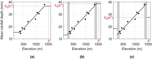
To summarize, in the last two cases (Figure 1b, c) an extrapolation is allowed up to a level e_max, while in the first one (Figure 1a) no extrapolation is allowed. In the third case (Figures 1c) marked discontinuities can appear when applying the constraint over a group of pixels, while in the first two cases (Figure 1a, b) discontinuities are not present. In all cases, extrapolation is not allowed when the elevation of the estimation cell is e_max higher than those of the rain gauges of the local sample.

In the subsequent Sections, we present the results obtained applying the different alternative constraints mentioned above. The final value for e_max is also defined after proper testing.

3. Application

According to what defined above, we approach to the analysis of the spatial variability of the average annual maxima in Italy through a local regression framework. The definition of the model configuration passes through the setting of the model configuration parameters introduced in Section 2. In this section, the parameter values are estimated for the Italian territory and a list of plausible model configurations is obtained.

3.1. Definition of the local sample

Italy has a ≈ 300,000 km² wide territory having marked mountainous characteristics (Figure 2a), that undermine the possibility of having a uniform rain gauge density. Even though an unprecedent rainfall data coverage is now available with the Improved Italian – Rainfall Extreme Dataset (Mazzoglio et al. 2020), the search for algorithms that predict extreme rainfall indices based on local data will face a marked spatial data heterogeneity in station density, with changes up to half an order of magnitude in different areas of the country.

Figure 2. Elevation data (a) and number of rain gauges available for each cell within a 15 km radius (b). Source: Shuttle Radar Topography Mission (Farr et al. 2007).

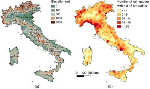
For each grid cell all over Italy we evaluated the number of rain gauges (with a time series of at least 10 years of data) available within circles with radius of 10, 15, 20 and 25 km. The results are shown in Table 1 in terms of the mean, median, modal and standard deviation values found.

Table 1. Mean, median, modal and standard deviation values of the rain gauges falling in circles of variable radius.

Radius (km)	Mean (n° of stations)	Median (n° of stations)	Mode (n° of stations)	Standard deviation (n° of stations)
10	3.9	3	2	2.7
15	8.2	7	5	5.2
20	14.3	13	7	8.4
25	21.8	19	14	12.2

The values shown in Table 1 are useful both to understand what could be a reasonable minimum local sample size n and to the selection of r. We then evaluated that a local sample of 5 stations within a 15 km radius can provide a reference set similar to the one used in PRISM (1 station every 3 km of radius in average).

More specifically, using a fixed 15-km radius we get a local sample of at least 5 rain gauges in over 227,150 grid cells (Figure 2b), leading to an equal minimum density in about 75% of Italy. As we do not consider reliable a regression fitted using a local sample with less than 5 values, for the remaining 25% of the cells over Italy we computed the average annual maxima using the 5 nearest stations, independently on their distance from the reference cell. It is interesting to note that the spatial coverage of this 25% of under-threshold density cells (that can be recognized as the yellow areas of Figure 2b) is quite coherent, i.e. cells are spatially connected. These areas often coincide with flat regions, where we expect a limited influence of the orographic effect. We decided not to reduce the radius because, if we consider as an example the case of 10 km, only 93,735 grid cells (≈ 31% of the Italian territory) can secure a local sample of at least 5 rain gauges.

Based on the results of Table 1, we considered model configurations with a fixed radius whose length is equal or greater than 15 km (r_fix = 15, 20 and 25 km), within which the criterion of pooling a minimum number of 5 stations was always kept valid.

For the variable radius approach, as described in Section 2.3, the radius length was allowed to vary between r_min = 1 km and r_max = 15 km to have a local regression. Some tests were performed using also larger r_max (up to 50 km) but we observed a marked decrease of the model performance, in terms of error statistics and residuals of the regressions, as the radius increases beyond 15 km. A quantitative estimation of the degradation of model performance is reported in Section 4.

3.2. Locally-averaged rainfall maps

As mentioned in Section 2.3, the estimation of the average annual maxima using the mean values of the n nearest stations can represent a strong reference for additional comparisons with all the other attempts based on more complex georegression models. In this case, no specific radius is used to put together a local sample whose spatial extension depends on the data density. This approach represents a step forward compared to the approach used in Mazzoglio et al. (2022), where geographical and geomorphological classifications were used to pool the data before fitting the model.

Figure 3a shows the average 1 h annual maxima computed on the basis of the n = 5 nearest stations: it can be seen that this approach does not allow to model the orographic gradients (i.e. some of the spatial patterns that follow the orography are missing) and several artifacts are clearly visible. Moreover, Figure 3b shows clusters of high residuals in correspondence of orographically complex areas as the Prealps.

Figure 3. Average annual maxima of 1 h duration computed on the basis of the 5 nearest stations (a). Residuals of the 1 h model, with an indication of the elevation (b). Box plots of measured and estimated mean of 1 h values (c).

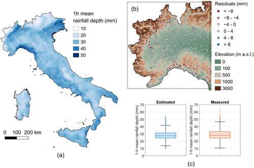
Figure 3c shows the comparison of the box plot of measured average values of the ≈ 3,800 time series with the reconstructed values of ≈ 300,000 pixels and confirms that a simple spatial averaging smooths the extremes: while the highest measured average annual maximum rainfall depth in 1 h is 64 mm, the highest estimated value is 54 mm. The analysis of the spatial distribution of the average annual maxima shows a concentration of high values in Liguria, North of Piedmont and Friuli Venezia Giulia. The reconstructed map, instead, shows a cluster of values > 50 mm only in Liguria, that incidentally shows a high density of rain gauges. In all the other regions, the rain gauges characterized by high values are sparse, and this probably justifies that the reconstructed average annual maxima are smoothed.

The results of Figure 3a suggests that, where possible, it is advisable to consider the links between rainfall and elevation with a georegression approach, using the bare local sample average as a baseline and as a surrogate of more accurate estimations when regressions are not possible.

3.3. Evaluation of parameters for model correction

3.3.1. Elevation range

To undertake the role of the elevation range of the sample we performed an analysis using the variable radius approach, without losing generality. For the analysis of this detail, moving from the results of Section 3.1, we referred to r_min = 15 km and r_max = 50 km and a minimum local sample size n = 5 to apply local regressions. We computed the rainfall gradient over elevation where possible, i.e. in the 75% of the Italian area and we checked the statistical significance and the spatial variability of the slope estimates. In terms of slope values, we noticed the presence of some consistent outliers in the box plots (see Figure 4). These very high values were mainly clustered in the flat areas, pointing to a data anomaly effect: we realized that an insufficient elevation range in the data sample was the reason of obtaining anomalously high (positive and negative) rainfall local gradient. Based on the experience gained in a previous work (Mazzoglio et al. 2022) and after some exploratory tests, we set the minimum Δz value to 100 m. Application of this constraint allowed us to remove a considerable number of outliers, as shown in Figure 4 (lower row of each subplot).

Figure 4. Visual representation through box plots of the slope coefficients obtained with a regression model based on r = 15 to 50 km and Δz = 0 or 100 m in the case of 1 (a) and 24 h durations (b). Please note that Δz is the minimum difference in elevation among the rain gauges of the local sample required to apply the regression.

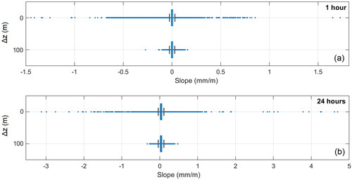
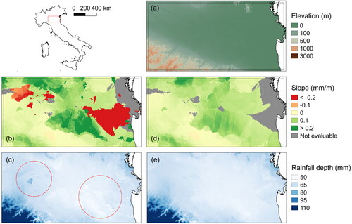
To support the assessment of the efficiency of the threshold criterion (Δz = 100 m), we tested its application comparing maps of estimated average annual maxima obtained without any constraint, to those built with the minimum range threshold Δz. Considering the average annual maxima in 24 h, the maps in Figure 5 show that, when assuming no threshold, several artifacts appear (see e.g. the dark triangle in the left part of Figure 5c). For reference, elevation data are visible in Figure 5a. In that area, slopes are obtained by applying the local regression to rain gauges presenting very similar elevations (say, with a 5–10 m elevation range only). Incidentally, the average rainfall depth presented moderate local variability (e.g. a 10 mm rainfall range). Applying, instead, the Δz = 100 m range threshold, we obtained more than reasonable improvements (Figure 5d, e) with removal of almost all artefacts. To verify the impact of using Δz = 100 m, among the proposed model configurations both cases with Δz = 100 m and Δz = 0 m are considered.

Figure 5. Elevation map with the indication of the area investigated (a). 24 h average annual maxima estimated using radii variable from 15 to 50 km (simulation with an extrapolation of 100 m allowed and with mean rainfall depth evaluated using the 5 nearest rain gauges in uncovered cells) in the case of Δz = 0 m (c) and Δz = 100 m (e) and related slope coefficients (b and d). Red circles in (c) serve to highlight artifacts. Grey color defines areas where the local regression approach is not applicable e.g. due to the impossibility of pooling at least 5 rain gauges or to the lack of significance of the regression model.

3.3.2. Extrapolation

Preliminary tests made on selected mountain areas showed the importance of considering constraints in applying the regression equation well beyond the elevation ranges of the local sample, as pointed out in Section 2.4. Extrapolation showed to produce even negative values of rainfall estimates in areas with complex topography. After a preliminary sensitivity analysis that proved that higher values degraded the model performances, the threshold value of e_max = 100 m was selected for the alternative constraints outlined in Section 2.4.

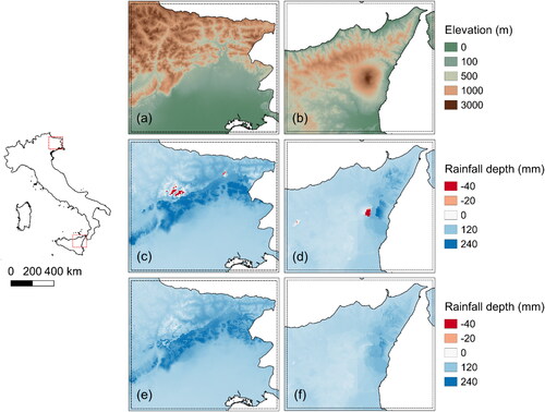
To exemplify, we have reported in Figure 6 the estimated values of the 24 h average annual maxima in two mountainous areas of Italy: in Friuli Venezia Giulia (Figure 6a, c and e) and in Sicily, near the Etna volcano (Figure 6b, d and f). In Figure 6e, f the estimates are obtained by selecting a maximum 100 m of extrapolation allowed. Figure 6c, d show the results obtained with the extrapolation allowed without limitations. Some cells with negative estimates appear in this latter case (the grid cells are highlighted in red in Figure 6c, d). The results in Figure 6e, f, obtained after correction, confirm that the extrapolation problem must be carefully handled. As mentioned in Section 2.4, we considered different limiting cases to tackle the problem. All three approaches to managing extrapolation presented in Section 2.4 are present in the model configurations examined to assess their impact.

Figure 6. Elevation data for Friuli Venezia Giulia (a) and Sicily (b). In (c, d) extrapolation is allowed without limits and red areas represent cells with negative estimated rainfall. In (e, f) extrapolation is limited to 100 m.

3.4. Selection of tested model configurations

As mentioned before, the geo-regression approach presented in this manuscript, even if simple, involves the selection of different parameters, namely the number of rain gauges that forms the local sample n, the elevation difference among the rain gauges of the local sample Δz, the area of support (r_fix, r_min, r_max) and the maximum extrapolation allowed e_max. On the basis of the analysis carried out in Section 3.1 to Section 3.4, meaningful combinations of the different parameters were applied and several techniques were jointly used to select the most valuable model. The most relevant model configurations considered in this study, in the following called Cases, are listed with their settings in Table 2.

Table 2. Most relevant model configurations.

Case	n (-)	Δz (m)	Radius configuration	rfix (km)	rmin (km)	rmax (km)	emax (m)	Extrapolation configuration (Section 2.4)
0	5	0	Variable	–	–	–	–	–
1	5	100	Variable (V1)	–	1	15	0	a
2	5	100	Variable (V1)	–	1	15	0	c
3	5	100	Variable (V2)	–	15	50	100	c
4	5	100	Fixed	15	–	–	100	b
5	5	100	Fixed	15	–	–	100	c
6	5	100	Fixed	20	–	–	100	c
7	5	100	Fixed	25	–	–	100	c

Case 0 represents the case with mean values reconstructed using the 5 nearest stations, while all the other tests were performed using georegression models. The last column refers to the configuration described in Section 2.4: in configuration ‘a’ extrapolation is not allowed while in ‘b’ and ‘c’ the extrapolation is allowed up to e_max (for the grid cells that would require extrapolation higher than e_max, in configuration ‘b’ the predicted value is set equal to the value obtained by the model at an elevation that is e_max higher/lower than those of the highest/lowest rain gauge of the sample, while in configuration ‘c’ the predicted value is computed using the 5 nearest stations).

As it can be seen, Case 0 is the model configuration where the evaluation of the average annual maxima is performed using the mean values of the 5 nearest stations all over the territory. Cases 1, 2 and 3 consider the variable radius approach, but with a difference if when reaching r_max the model pools together at least 5 rain gauges and the regression is not statistically significant: Case 1 and Case 2 applied the model without considering the p-value (Variable (V1)); Case 3 used the mean rainfall value evaluated using the 5 nearest stations (Variable (V2)).

Cases 4, 5, 6 and 7 refer to the fixed radius approach, for two different extrapolations configurations and three radii: 15, 20 and 25 km.

4. Discussion of results and rainfall maps

4.1. Residual analysis and model selection

To evaluate the performance of the cases listed in Table 2, we carefully analyzed the residuals. For each case two sets of residuals were analyzed: (i) the residuals obtained from a cross-validation (leave-one-out approach), that is ‘cross-validation configuration’ and (ii) the residuals obtained applying the regression on the whole data, that is ‘real model configuration’.

As a first step, error statistical indexes were computed for each residual set: bias, mean absolute error (MAE), root mean square error (RMSE) and Nash-Sutcliffe model efficiency coefficient (NSE) (Nash and Sutcliffe 1970; Wasserman 2004).

Results obtained for the 1 h duration are reported in Table 3 for the cross-validation configuration and in Table 4 for the real model configuration. Similarly, for the 24 h duration, the results of the cross-validation configuration are reported in Table 5 while the real model configuration is summarized in Table 6. The results shown in Tables 3 to 6 do not clearly indicate a model that is able to outperform all the others. Moreover, 1- and 24-hour durations seem to perform differently. As expected, Cases 3, 6 and 7 that consider a large radius do not perform well because the benefit of working with a local sample is lost. Focusing on short radii (Cases 1, 2, 4 and 5), comparable performances of the models emerged. For the 1 h duration, as an example, the fixed radius case with r_fix = 15 km (Case 5) performs slightly better in cross-validation mode (Table 3) but considering the performance of the real model (Table 4), the variable radius approach (Cases 1 and 2) proved to be better, even if the improvement in terms of error statistics is limited.

Table 3. Results of the cross-validation configurations for the 1 h duration.

Statistic	Case 0	Case 1	Case 2	Case 3	Case 4	Case 5	Case 6	Case 7
BIAS (mm)	−0.11	0	−0.02	−0.01	−0.02	−0.03	−0.02	−0.01
MAE (mm)	3.13	3.12	3.14	3.34	3.11	3.10	3.14	3.21
RMSE (mm)	4.15	4.12	4.17	4.43	4.12	4.10	4.15	4.26
NSE (-)	0.68	0.68	0.68	0.64	0.69	0.69	0.68	0.66
NRG (-)	223	222	230	263	221	214	216	234

Table 4. Results of the real model configurations for the 1 h duration.

Statistic	Case 0	Case 1	Case 2	Case 3	Case 4	Case 5	Case 6	Case 7
BIAS (mm)	−0.07	−0.01	−0.02	−0.03	−0.03	−0.03	−0.03	−0.01
MAE (mm)	2.51	2.57	2.56	2.95	2.60	2.60	2.78	2.96
RMSE (mm)	3.35	3.44	3.43	3.96	3.48	3.48	3.70	3.94
NSE (-)	0.79	0.78	0.78	0.71	0.77	0.77	0.75	0.71
NRG (-)	101	118	117	189	122	122	151	184

Table 5. Results of the cross-validation configurations for the 24 h duration.

Statistic	Case 0	Case 1	Case 2	Case 3	Case 4	Case 5	Case 6	Case 7
BIAS (mm)	−0.66	−0.14	−0.25	−0.25	−0.14	−0.06	0.10	0.07
MAE (mm)	10.17	10.38	10.51	11.04	10.45	10.37	10.84	11.46
RMSE (mm)	14.87	15.40	15.69	16.61	15.56	15.40	16.22	17.21
NSE (-)	0.79	0.78	0.77	0.74	0.77	0.78	0.75	0.72
NRG (-)	207	219	236	275	225	218	250	280

Table 6. Results of the real model configurations for the 24 h duration.

Statistic	Case 0	Case 1	Case 2	Case 3	Case 4	Case 5	Case 6	Case 7
BIAS (mm)	−0.48	−0.26	−0.21	−0.37	−0.14	−0.14	−0.01	0.10
MAE (mm)	8.14	8.47	8.35	9.64	8.68	8.68	9.64	10.61
RMSE (mm)	12.02	12.76	12.53	14.81	13.10	13.10	14.61	16.08
NSE (-)	0.86	0.85	0.85	0.79	0.84	0.84	0.80	0.76
NRG (-)	116	138	129	193	142	142	192	240

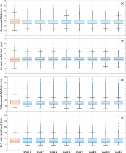
For an accurate analysis of the residuals, we also analyzed the box plots of the reconstructed values for both the ‘real model configuration’ and the ‘cross-validation configuration’ (Figure 7), compared with the box plot of measured values. Figure 7 shows that models based on variable radii (with an upper threshold of 15 km, i.e. Cases 1 and 2) proved to be able to cover almost the same measurement range of the measured values. Measured values have higher upper quartile and maximum whiskers, but the median values remain almost constant.

Figure 7. Box plots of the real model configurations for the 1 h (a) and 24 h (c) durations and box plots of the cross-validation configurations for the 1 h (b) and 24 h (d) durations. The orange box plots refer to the measured values, while the blue box plots refer to the estimated value.

Thornton et al. (2021) pointed out that unrealistically high estimated rainfall values can be obtained using a local-regression approach. In their approach, if the estimated rainfall depth is more than twice the highest measured rainfall depth, this anomalous value is reduced to twice the maximum measured rainfall depth. By applying constraints on the search radius and on the extrapolation, we never encountered this problem, independently on the duration that we considered.

A close inspection of the residuals and their spatial aggregation was also performed (not reported here for brevity). The analysis of the spatial distribution of the residuals confirms what was outlined in Section 2.3: for the variable radius configuration, by increasing both r_min and r_max the benefit of using a local regression approach decreases. Case 3, with r_min = 15 km and r_max = 50 km, presents larger clusters, and significant residuals with opposite signs lying at close distances. By comparing the data density map (Figure 2) with the maps of the cross-validation residuals (not reported here for brevity) it emerges that the largest errors are in areas with complex topography and low instrument density. This fact suggests that, even with a high data density, some local behaviors were not correctly represented and managed with the proposed approach when too large area were considered in the regression model. The higher spatial homogeneity of residuals in the case of smaller variable radii or fixed radius suggests that these models should be preferable, keeping in mind that even with this configuration some high local errors remain.

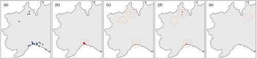
To have a complete picture of the model configurations of Table 2, we focused also on the estimation of the average annual maxima, following what emerged in Section 3.2. As an example, Figure 8a shows the location of the rain gauges with a 1 h average annual maximum of at least 50 mm while Figure 8b to e shows the location of the estimated values for Case 0, Case 1, Case 2 and Case 5. As it can be seen in Figure 8b a simple computation of the average annual maxima performed by using the 5 nearest rain gauges (Case 0), even if providing good error metrics, cannot reconstruct the extremes in the northern part of the area. Conversely, a model based on a georegression, as Cases 1 and 2, provides additional information, even if the area where we expect to reach high rainfall depths shows some underestimated values (Figure 8c, d). Model 5, despite good performance, is not able to reconstruct the extremes and, in addition, it overestimates the average annual maxima in the North-East of the area (Figure 8e).

Figure 8. Spatial distribution of the rain gauges with 1 h average annual maxima higher than 50 mm (a). Location of the estimated values higher than 50 mm for Case 0 (b), Case 1 (c), Case 2 (d) and Case 5 (e).

By integrating all the above features, we suggest that the model configuration of Case 1 represents the best compromise and can be taken as the optimal model for all the durations.

4.2. Orographic gradients and rainfall maps

4.2.1. Orographic gradients

By varying the model parameters, only minor differences in the sign of the orographic gradients emerge, but the general picture remains. Thus, for the best model configuration considered in Section 4.1 (Case 1), it can be worth examining the spatial variability of the slope coefficients emerged by the regression models. These have been mapped in Figure 9 and represent an answer to the scientific question regarding the sign of the orographic effect on extreme rainfall.

Figure 9. Slope coefficients of the regression models for the 1 h (a) and 24 h (b) duration in the case of r = 1 to 15 km.

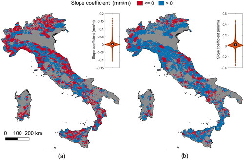
As introduced in Mazzoglio et al. (2022), the orographic effect (rainfall gradient with elevation) appears to vary greatly with the duration of the extreme rainfall in Italy. In Figure 9a we show the gradient for the 1 h duration average annual maxima. The grey color is used for the areas where the regression model cannot be applied due to low data density or extrapolation constraints. Over most of the Alps, Liguria region and portions of the Apennines, a general decrease of the 1 h average annual maxima with increasing elevation emerges (confirming thus the ‘reverse orographic effect’ mentioned in Allamano et al. (2009), in Avanzi et al. (2015), in Formetta et al. (2022) and in Mazzoglio et al. (2022)), while over most of the hills, pre-hills and flat areas, the average annual maxima increases with the elevation.

Figure 9b shows the slope coefficients for the 24 h duration, for the same model configurations. The maps confirm a general increase of the 24 h average annual maxima with increasing elevation over Italy, except for some hill/mountainous areas.

4.2.2. Extreme rainfall maps of Italy

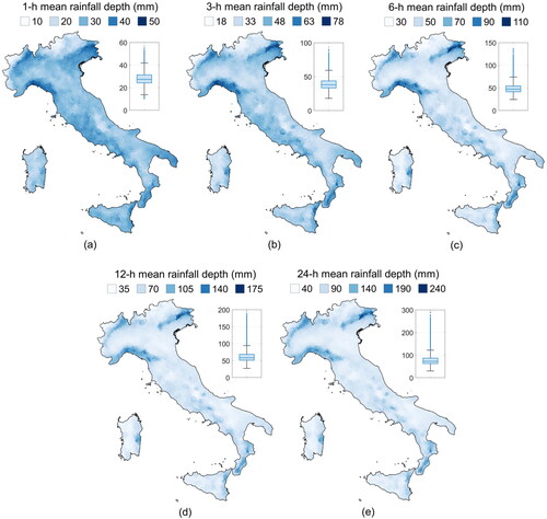
The optimal model configuration, Case 1, is used to evaluate the average annual maxima over Italy, as reported in Figure 10. For short durations (e.g. for the 1 h interval, depicted in Figure 10a) the Northern areas of Aosta Valley and Bolzano province exhibited average annual maxima smaller than in Southern Italy. For longer durations (e.g. for the 24 h interval, Figure 10e), these areas are affected by a mean rainfall depth comparable with the one recorded in Sicily and Sardinia Islands, in the Po Valley and in the Southern Apennines. The wetter areas are located in Friuli Venezia Giulia, in Liguria, in the northern areas of Piedmont and in Calabria. It is interesting to notice that the 1- and 24-hour durations have different characteristics: as the duration increases, the highest values appears to be clustered in space and focused over limited areas.

Figure 10. Average annual maxima for 1 (a), 3 (b), 6 (c), 12 (d) and 24 (e) hour intervals and related box plots.

5. Conclusions

In this work we propose an improved local regression approach to describe the spatial variability of the average annual maximum rainfall depths for short durations (1, 3, 6, 12 and 24 h) over Italy. The proposed method optimizes the interpolation through the selection of small samples that emphasize the value of high local station density. The application of the proposed method allows to highlight the presence of several areas with negative orographic gradients in Italy. The optimal regression model configuration was selected by analyzing the residuals through cross-validations, through visual inspection of their spatial distributions and adding a comparative analysis of their box plots. With regard to Italy, the results presented in Section 4 suggest that the estimation of the average annual maxima using a local regression in each considered pixel, calibrated for a limited spatial extent (circle with radius of 15 km at maximum) represents the solution that best preserves the local features of the regressions in relation to very variable data densities over the entire country, as explained in Section 4.1.

In the development of the regression model particular attention was paid to the presence of artifacts, that appear to depend on non-consistent rainfall gradients or to extrapolation issues. Different to the Daymet model (Thornton et al. 2021), in our work negative gradients are not considered errors and are not equaled to zero, but their values are only controlled through appropriate constraints on data elevation range. In addition, our analysis showed that the model performance gets worse when the regression model is applied at elevations outside the elevation range of the data used for the regression. To avoid this drawback, we suggested setting the predicted value as the value obtained by the model in correspondence of the elevation of the highest/lowest rain gauge used in the regression model.

Through the proposed approach, the obtained maps of average annual maxima clearly show that even wide areas are subject to a decrease in sub-daily rainfall maxima with elevation.

The maps and the methodological results presented in this work, that mainly regard the analysis of the spatial variability of orographic gradients, provide a baseline that can be important in view of regional rainfall frequency analyses, aimed to estimate high return period rainfall quantiles. The same knowledge, for the first time extended to the whole of Italy, will help to investigate the different morphological/climatological characteristics that lead to orographic effects, that can play a significant role in catchment-based hydrological analyses.

Acknowledgements

The authors acknowledge the regional agencies involved in the management of the rain gauge networks that provided the rainfall measurements included in I²-RED. Full credits are reported in Mazzoglio et al. (2020).

Disclosure statement

The authors report that there are no competing interests to declare.

Data availability statement

Although Italian law requires an open-source policy for all public data, this right has not yet been implemented by all the Italian agencies involved in the management of the rain gauge network. The agreements we signed with some of these agencies, aimed at monitoring the correct use of the data, restricted their use to the aims of the authors’ project. As a result of these legal restrictions, a complete version of I²-RED can only be provided to two groups of people: members of the authors’ research group (who are already fully authorized to use the data) and people who can prove they have received clearance from the regional authorities. The entire quality-controlled database is available on Zenodo (https://doi.org/10.5281/zenodo.4269509), albeit with restricted access. The data can be used by third parties, for an indefinite timeframe, upon having completed an agreement with the authors and with the regional agencies involved in the data collection. The raw data availability depends on the region: a complete description of how to access these data is reported in Mazzoglio et al. (2020).

References

- Allamano P, Claps P, Laio F, Thea C. 2009. A data-based assessment of the dependence of short-duration precipitation on elevation. Phys Chem Earth. 34: JPCE1649.
- Avanzi F, De Michele C, Gabriele S, Ghezzi A, Rosso R. 2015. Orographic signature on extreme precipitation of short durations. J Hydrometeorol. 16(1):278–294.
- Basist A, Bell GD, Meentemeyer V. 1994. Statistical relationships between topography and precipitation patterns. J Clim. 7(9):1305–1315.
- Brunsdon C, McClatchey J, Unwin D. 2001. Spatial variations in the average rainfall–altitude relationship in Great Britain: an approach using geographically weighted regression. Int J Climatol. 21(4):455–466.
- Claps P, Ganora D, Mazzoglio P. 2022. Rainfall regionalization techniques. In: Morbidelli R, editor. Rainfall. Elsevier; p. 327–350.
- Crespi A, Brunetti M, Lentini G, Maugeri M. 2018. 1961–1990 high-resolution monthly precipitation climatologies for Italy. Int J Climatol. 38:878–895.
- Crespi A, Brunetti M, Ranzi R, Tomirotti M, Maugeri M. 2021. A multi-century meteo-hydrological analysis for the Adda river basin (Central Alps). Part I: gridded monthly precipitation (1800–2016) records. Int J Climatol. 41(1):162–180.
- Daly C, Neilson RP, Phillips DL. 1994. A statistical-topographic model for mapping climatological precipitation over mountainous terrain. J Appl Meteor. 33(2):140–158.
- Daly C, Gibson WP, Taylor GH, Johnson GL, Pasteris P. 2002. A knowledge-based approach to the statistical mapping of climate. Clim Res. 22(2):99–113.
- Daly C. 2006. Guidelines for assessing the suitability of spatial climate data sets. Int J Climatol. 26(6):707–721.
- Dalrymple T. 1960. Flood-frequency analyses. manual of hydrology: part 3. Floodflow techniques. Technical report, United States Government Printing Office, Washington (United States).
- Di Piazza A, Lo Conti F, Noto LV, Viola F, La Loggia G. 2011. Comparative analysis of different techniques for spatial interpolation of rainfall data to create a serially complete monthly time series of precipitation for Sicily, Italy. Int J Appl Earth Obs Geoinf. 13(3):396–408.
- Diodato N, Ceccarelli M. 2005. Interpolation processes using multivariate geostatistics for mapping of climatological precipitation mean in the Sannio Mountains (southern Italy). Earth Surf Process Landforms. 30:259–268.
- Farr TG, Rosen PA, Caro E, Crippen R, Duren R, Hensley S, Kobrick M, Paller M, Rodriguez E, Roth L, et al. 2007. The shuttle radar topography mission. Rev Geophys. 45(2):RG2004.
- Formetta G, Marra F, Dallan E, Zaramella M, Borga M. 2022. Differential orographic impact on sub-hourly, hourly, and daily extreme precipitation. Adv Water Resour. 159:104085.
- Fotheringham S, Brunsdon C, Charlton M. 2002. Geographically weighted regression: the analysis of spatially varying relationships. Chickester (UK): Wiley.
- Fowler HJ, Wasko C, Prein AF. 2021a. Intensification of short-duration rainfall extremes and implications for flood risk: current state of the art and future directions. Philos Trans A Math Phys Eng Sci. 379(2195):20190541.
- Fowler HJ, Lenderink G, Prein AF, Westra S, Allan RP, Ban N, Barbero R, Berg P, Blenkinsop S, Do HX, et al. 2021b. Anthropogenic intensification of short-duration rainfall extremes. Nat Rev Earth Environ. 2(2):107–122.
- Frei C, Schär C. 1998. A precipitation climatology of the Alps from high-resolution rain-gauge observations. Int J Climatol. 18:873–900.
- Golzio A, Crespi A, Bollati IM, Senese A, Diolaiuti GA, Pelfini M, Maugeri M. 2018. High-resolution monthly precipitation fields (1913–2015) over a complex mountain area centred on the Forni Valley (Central Italian Alps). Adv Meteorol. 2018:9123814.
- Goovaerts P. 1999. Using elevation to aid the geostatistical mapping of rainfall erosivity. Catena. 34(3–4):227–242.
- Isotta FA, Frei C, Weilguni V, Tadic MP, Lassegues P, Rudolf B, Pavan V, Cacciamani C, Antolini G, Ratto SM, et al. 2014. The climate of daily precipitation in the Alps: development and analysis of a high-resolution grid dataset from pan-alpine rain-gauge data. Int J Climatol. 34(5):1657–1675.
- Libertino A, Allamano P, Laio F, Claps P. 2018. Regional-scale analysis of extreme precipitation from short and fragmented records. Adv Water Resour. 112:147–159.
- Libertino A, Ganora D, Claps P. 2019. Evidence for increasing rainfall extremes remains elusive at large spatial scales: the case of Italy. Geophys Res Lett. 46(13):7437–7446.
- Mazzoglio P, Butera I, Claps P. 2020. I2-RED: a massive update and quality control of the Italian annual extreme rainfall dataset. Water. 12(12):3308.
- Mazzoglio P, Butera I, Alvioli M, Claps P. 2022. The role of morphology in the spatial distribution of short-duration rainfall extremes in Italy. Hydrol Earth Syst Sci. 26(6):1659–1672.
- Mazzoglio P, Ganora D, Claps P. 2022. Long-term spatial and temporal rainfall trends over Italy. Environ Sci Proc. 21:28.
- Nash JE, Sutcliffe JV. 1970. River flow forecasting through conceptual models part I—A discussion of principles. J Hydrol. 10(3):282–290.
- Pellicone G, Caloiero T, Modica G, Guagliardi I. 2018. Application of several spatial interpolation techniques to monthly rainfall data in the Calabria region (southern Italy). Int J Climatol. 38(9):3651–3666.
- Prudhomme C, Reed DW. 1998. Relationships between extreme daily precipitation and topography in a mountainous region: a case study in Scotland. Int J Climatol. 18(13):1439–1453.
- Prudhomme C, Reed DW. 1999. Mapping extreme rainfall in a mountainous region using geostatistical techniques: a case study in Scotland. Int J Climatol. 19(12):1337–1356.
- Thornton PE, Running SW, White MA. 1997. Generating surfaces of daily meteorological variables over large regions of complex terrain. J Hydrol. 190:214–251.
- Thornton PE, Shrestha R, Thornton M, Kao SC, Wei Y, Wilson BE. 2021. Gridded daily weather data for North America with comprehensive uncertainty quantification. Sci Data. 8(1):190.
- Wasserman L. 2004. Models, statistical inference and learning. In: Wasserman L, editor. All of statistics. New York (NY): Springer; p. 87–96.