Combination four different ensemble algorithms with the generalized linear model (GLM) for predicting forest fire susceptibility

Abstract

In this study, the generalized linear model (GLM) and four ensemble methods (partial least squares (PLS), boosting, bagging, and Bayesian) were applied to predict forest fire hazard in the Chalus Rood watershed in the Mazandaran Province, Iran. Data from 108 historical forest fire events collected through field surveys were applied as the basis of the analysis. About 70% of the data were used for training the models, while the remaining 30% was used for testing. A total of 14 environmental, climatic, and vegetation variables were used as input features to the models to predict forest fire probability. After conducting a multicollinearity test on the independent variables, the GLM and the ensemble models were applied for modeling. The efficiency of the models was evaluated using receiver operating characteristic (ROC) curve parameters. Results from the validation process, based on the area under the ROC curve (AUC), showed that the GLM, PLS-GLM, boosted-GLM, Bagging-GLM, and Bayesian-GLM models had efficiencies of 0.79, 0.75, 0.81, 0.84, and 0.85, respectively. The results indicated that all ensemble methods, except the PLS algorithm, improved the performance of the GLM model in modeling forest fire hazards in the Chalus Rood watershed, with the Bayesian algorithm being the most efficient method among them.

Keywords:

• Generalized linear model
• ensemble
• natural hazards
• Chalus Rood watershed
• forest fire susceptibility
• artificial intelligence
• mathematics

1. Introduction

Forest fires are a crucial environmental problem under ongoing climate change, which threaten human lives and the environment (Huebner et al. 2012). Forest fires affect the pattern of forest formation (Huesca et al. 2009). Many factors, such as temperature, rainfall, drought, and human activity, can influence the frequency and intensity of forest fire (Eastaugh & Hasenauer 2014). Forest fires are also damaging and destructive natural disasters, triggering significant fatalities and economic loss every year (Kwak et al. 2012). Forest fire susceptibility modeling plays a critical role in forest management and conservation efforts (Chicas and Østergaard Nielsen 2022). Accurate prediction of forest fires is vital for the sustainable management of forests and planning of emergency procedures by local authorities (Tehrany et al. 2019).

Statistical and physics-based models have been employed to model the forest fire susceptibility (Pourtaghi et al. 2015; Agranat and Perminov 2020; Lattimer et al. 2020; Chicas and Østergaard Nielsen, 2022; Das et al. 2023). Statistical models utilize past fire data to predict fire occurrences (Das et al. 2023). Statistical methods are restricted by assumptions about the data and may struggle to robustly capture complex relationships among variables (Jain et al. 2020). They may not be able to robustly capture intrinsic nonlinearity and nonstationary between the forest fire signature and predictor variables, and thus they perform poorly (Chicas and Østergaard Nielsen, 2022). These models also cannot account for cross correlation between variables. It is a common practice to assume the regression residuals are normally distributed, but this may not be a valid assumption (Tang et al. 2020). Furthermore, statistical models require many data to estimate the behaviour of unknown systems (Bui et al. 2017).

Physical-based models incorporate physical properties such as weather and topography to estimate fire behaviour and spread (Collin et al. 2011). They are good at providing insights into catchment environmental processes, but they have been criticized for being uncertain and difficult to implement (Zheng et al. 2017). With complex model structures and extensive calculation requirements, physical-based forest fire models often have high computational costs and require high levels of environmental expertise for modellers and users, thus limiting their application in forest fire management (Chew et al. 2022). Also, physical models often require a significant effort and many environmental variables for calibration in order to simulate physical processes of the watershed (Reinhardt et al. 2001). On the other hand, physics-based models require detailed information on various factors that may not be easily accessible, particularly in remote or inaccessible regions (Jain et al. 2020).

In a departure from statistical and physical models, machine learning (ML) approaches have emerged as a powerful tool for forest fire susceptibility modeling due to their ability to handle large and complex datasets, and to learn patterns and relationships from data automatically (Shahfahad et al. 2022; Saha et al. 2023). Recently, ML algorithms were utilized to model forest fires in different locations (Pourghasemi et al. 2020; Talukdar et al. 2022). The commonly used ML approaches for modeling forest fires are support vector machine (SVM, Gonzalez-Olabarria et al. 2012; Bera et al. 2022a), artificial neural network (ANN, Pang et al. 2022), deep learning network (DLN, Saha et al. 2023), random forest (RF, Rubí et al. 2023), boosted regression tree (BRT, Kalantar et al. 2020), logistic model trees (LMT, Reyes-Bueno and Loján-Córdova, 2022), extreme gradient boosting (XGBoost, Akıncı and Akıncı, 2023), Bayes network (BN, Pham et al. 2020), multivariate adaptive regression splines (MARS, Tien et al. 2019), and generalized linear model (GLM, Eskandari et al. 2020b; Pourghasemi et al. 2020).

Recent studies in environmental hazard modeling have shown that ensembles of multiple ML algorithms tend to outperform individual algorithms (Ahmadi et al. 2020; Band et al. 2020a, 2020b; Kalantar et al. 2020; Shao et al. 2023). The GLM remains a valuable tool for fire susceptibility mapping. It also has been widely used to identify relationships between independent and dependent variables for fire management and planning (Carvalho et al. 2018 ; Ríos-Pena et al. 2017). In the context of GLM for spatial modeling, the accuracy of results can be improved by combining ensemble methods with GLMs. This is particularly important because the estimation of forest fire risk is complex owing to the multiple interactions of the factors that affect the ignition phenomena. The four most commonly used ensemble methods in spatial modeling are Bayesian, Bagging, Boosting, and partial least squares (PLS). Each of these approaches has its own strengths and drawbacks and can be used depending on the particular goals and requirements of the study. Bayesian allows incorporating prior knowledge and estimating uncertainties of the GLM (Tran et al. 2020). Bagging can reduce the variance and increases stability of results from the GLM (Sutton, 2005). Boosting can reduce the bias and variance of predictions from the GLM (Bou-Hamad et al. 2017). Finally, PLS can improve interpretability and computational efficiency of the GLM (Ding and Gentleman 2005).

Although these ML models are efficient in predicting the forest fire susceptibility, their accuracy is still debated. Previous studies have shown that there is no reliable framework for selecting multiple algorithms to model the forest fire susceptibility (Abedi et al. 2021; Achu et al. 2021). The complex interaction between various factors that contribute to forest fire ignition and spread makes it challenging to accurately model and predict forest fires over regional scales. Furthermore, the uncertainty in inter-model predictions yields an unclear decision-making process (Bui et al. 2016; Gigović et al. 2019). This paper proposes the use of four hybrid ML methods, namely PLS-GLM, Boosted-GLM, Bagging-GLM, and Bayesian-GLM for modeling forest fire susceptibility, with the aim of improving the accuracy of forest fire prediction. To the best of our knowledge, there has been no prior attempt to use these four ensemble methodologies in combination with the GLM for modeling forest fire susceptibility.

The main aim of this study is to assess the efficiency of four ensemble algorithms (i.e. PLS, Bagging, Boosting and Bayesian) to augment the ability of the GLM model in predicting forest fire hazards. The secondary aim of this work is to produce accurate forest fire maps in the Chalus Rood watershed in Mazandaran Province (Iran) as they are crucial for informed and effective forest management practices. The application of advanced ML methods in the forest fire simulation provides valuable insights into the behaviour and spread of fires under different conditions in the Chalus Rood watershed. This is particularly important because forest fires in this watershed have far-reaching and long-lasting impacts on the local communities. Furthermore, by providing an augmented understanding of the causes and consequences of forest fires in this region, these models can support sustainable forest management practices and help to prevent future forest fires.

2. Study area and data

2.1. Study area

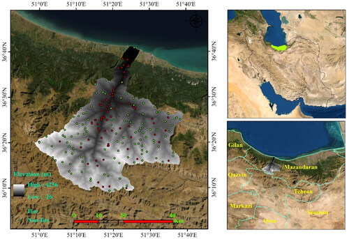
Forest fires are a common occurrence in the Chalus Rood watershed from May to December, mainly due to declining humidity levels and higher wind speeds. However, most of fires are initiated by human activities such as intentional burning for agriculture and campfires. In Mazandaran Province, some forest areas have been devastated by fires due to high temperatures and reduced precipitation, which dramatically increase the risk of fires and change their behaviour. Therefore, prediction and preparing forest fire maps are needed to recognize critical areas. The Chalus Rood watershed is a part of the Caspian Sea basin, which has 18 sub-watersheds (50°58′–51°40′ E and 36°08′–36°36′ N) with an area of ∼1634 km² located in Mazandaran Province, Iran (Figure 1). The maximum and minimum altitudes of the Chalus Rood watershed are 4256 and −26 m above sea level, respectively. The area is mountainous, with a steep slope towards the north. The region mainly experiences cold and humid climate, with semi-arid cold conditions in some lowlands. The annual rainfall in the study area varies from 288.3 mm to 1538.2 mm. Precipitation is seasonal and mainly occurs during winter and autumn. Land use in the study area included forests (dominant), pastures, agriculture, and gardens. The forests in the study area (Caspian) are a remnant of the third geological period with many species of that period existing in them (Kalantar et al. 2020). In recent years, fires in the Chalus Rood basin have caused the destruction of forestlands, most of which occurred in the summer and were human-induced.

Figure 1. Location of the study area: a) Iran, b) Mazandaran Province, and c) Chalus Rood watershed.

2.2. Forest fire inventory map

The Department of Natural Resources in the Province of Mazandaran collected forest fires in the Chalus Rood watershed from 2006 to 2018 through field surveys (https://frw.ir/). We used a total of 108 forest fire data points in the study domain during 2006–2018. These points represent the center of burned areas. On the basis of available forest fire data in the study domain, the period 2006–2018 was utilized for mapping forest fire susceptibility. To generate non-fire points, a circular buffer zone with a diameter of 400 m was created around each forest fire location utilizing the Buffer module in ArcGIS 10.5 software. Outside these buffer zones, 108 non-fire points were randomly selected. A similar approach was employed by Yaakob et al. (2011), Tomar et al. (2021), and Mabdeh et al. (2022) to generate non-forest fire points.

2.3. Dataset

The selection of factors influencing forest fire mapping was based on a review of previous studies (Eastaugh & Hasenauer 2014; Hong et al. 2018; Jaafari et al. 2019) and data availability. Totally, 14 variables were chosen in this research: elevation, aspect, curvature, slope, distance from river, distance from residential area, distance from road, land use, normalized difference moisture index (NDMI), land surface temperature (LST), soil-adjusted vegetation index (SAVI), normalized difference vegetation index (NDVI), rainfall, and temperature. The integration of maps depicting these factors and related thematic layers was performed by ArcGIS 10.5, SAGA GIS, and ENVI 5.1 (Table 1 and Figure 2).

Figure 2. Forest fire influencing factors: (a) altitude, (b) aspect, (c) slope, (d) curvature, (e) distance from river, (f) distance from road, (g) distance from residential area, (h) Land use, (i) LST, (j) NDMI, (k) NDVI, (l) SAVI, (m) rainfall, and (n) temperature.

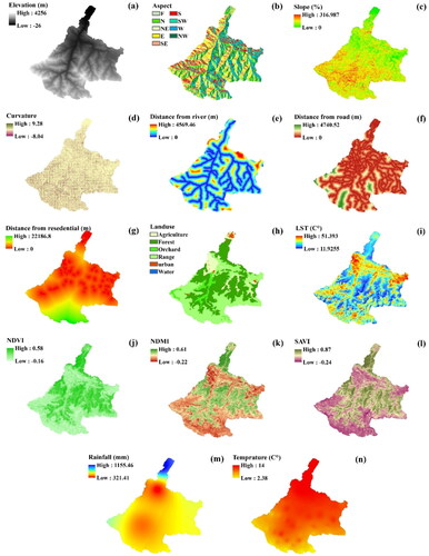
Table 1. Data type, source, and resolution of the independent variables.

Variables	Data type	Data source	Data resolution
Elevation	Raster Grid	Shuttle Radar Topography Mission (SRTM)	30 × 30 m
Aspect
Slope
Curvature
Distance from River	Line and polygon coverage	Administration of Natural Resources Department, Mazandaran Province.	1:50,000
Distance from Road	Line and polygon coverage	Administration of Natural Resources Department, Mazandaran Province.	1:50,000
Distance from residential	polygon coverage	LULC	30-m spatial resolution
LULC	Spatial/Raster grid	Landsat 8 OLI (USGS)	30-m spatial resolution
LST	Spatial/Raster grid	Landsat 8 OLI (USGS) Band 10 and Band 11	30-m spatial resolution
NDVI	Spatial/Raster grid	Landsat 8 OLI (USGS) Band 4 and Band 5	30-m spatial resolution
NDMI
SAVI
Rainfall	Station specific information	25-year information of rain gage stations	Interpolation with the same spatial resolution with other parameters
Temperature	Station specific information	25-year information of climatology stations	Interpolation with the same spatial resolution with other parameters

Topographical variables play a significant role in the initiation and growth of forest fires (Tariq et al. 2021). Elevation directly affects temperature, moisture, and wind patterns, and thus it is a crucial factor in fire propagation (Jaiswal et al. 2002). Although fires tend to be milder at higher altitudes because of increased rainfall (Adab et al. 2013), slope can significantly impact the fire spread rate. Fires move more rapidly uphill than downhill (Pourtaghi et al. 2015), and slope has a higher influence on fire spread than elevation. The direction of the slope (aspect) also affects forest fires as it controls the amount of solar energy received in the area. In the North Hemisphere, south-facing slopes receive more solar radiation and thus have a higher temperature, less humidity, and drier vegetation, which enhance the likelihood of ignition (Prasad et al. 2006; Setiawan et al. 2004). Curvature, or the degree of bending, of a terrain surface can have a significant impact on forest fires. A positively curved (convex) surface can trap and concentrate heat, wind, and fire, leading to increased fire intensity and spread. Conversely, a negatively curved (concave) surface can interrupt the flow of wind and fire, helping to slow down and contain the fire (Pourghasemi, 2016).

The Shuttle Radar Topography Mission (SRTM) digital elevation model (DEM) with a spatial resolution of 30 m was downloaded from the USGS EarthExplorer website (https://earthexplorer.usgs.gov/) for our case study. The elevation, slope, curvature, and aspect maps were produced based on the DEM using ArcGIS 10.5. Land use can significantly influence the frequency and severity of forest fires. Human activities such as agriculture and urbanization practices can increase the likelihood of fire ignition and growth (Kant Sharma et al. 2012; Nuthammachot and Stratoulias, 2021). The land use map was generated from a Landsat 8 OLI satellite imagery captured on 21st July 2019 using the maximum likelihood method in ENVI 5.1.

 Vegetation indices play an important role in understanding and predicting forest fires. These indices provide information about the health, density, and moisture content of vegetation. Normalized Difference Vegetation Index (NDVI) is widely used to monitor the status of plants, and is given by (Cheret and Denux, 2011; Digavinti and Manikiam, 2021), (1) $$\mathrm{NDVI}=\left(\mathrm{NIR}\text{-}\mathrm{Red}\right)/(\mathrm{NIR}+\mathrm{Red}),$$(1) where NIR and Red represent the near-infrared and red bands, respectively. NDVI varies from −1 to 1. High NDVI values indicate healthy, dense, and moist vegetation, while low values indicate unhealthy, sparse, and dry vegetation, which is more susceptible to ignition and spread of fire (Chuvieco et al. 2004; Abdo et al. 2022).

Normalized Difference Moisture Index (NDMI) is another vegetation index employed to evaluate the moisture of vegetation (Taloor et al. 2021; Abdo et al. 2022). It is calculated by, (2) $$\mathrm{NDMI}=\frac{\mathrm{NIR}\text{-}\mathrm{SWIR}}{\mathrm{NIR}+\mathrm{SWIR}},$$(2) where SWIR is the short-wave infrared band. Positive values of NDMI indicate high moisture content in vegetation, while negative values indicate low moisture content and dry vegetation (Taloor et al. 2021; Abdo et al. 2022).

The Soil-Adjusted Vegetation Index (SAVI) is a vegetation index that is adjusted for the effect of soil background on the reflectance measurement. It can be calculated by, (3) $$\mathrm{SAVI}=\left(\mathrm{NIR}\text{-}\mathrm{Red}\right)\times (1+L)/(1+L),$$(3) where L is a correction factor (between 0 and 1) that adjusts for the soil background influence. A value of L = 0.5 is commonly used (Vargas-Cuentas and Roman-Gonzalez, 2021).

The NDVI, NDMI, and SAVI were derived from the same Landsat 8 OLI satellite imagery by ENVI 5.1 (Table 1).

Land surface temperature (LST) has a significant effect on the occurrence and spread of forest fires (Maffei et al. 2018). Higher LSTs tend to dry out fuels and reduce the moisture content of vegetation, making them more vulnerable to ignition. LST can also impact atmospheric stability and wind patterns, further affecting fire behaviour. Thus, understanding the relationship between LST and forest fires is imperative for improving fire management and mitigating the risks of fires (Ahmed et al. 2020). The LST was computed based on bands 10 and 11 of the Landsat satellite images by the ENVI software (Ahmed et al. 2020). This algorithm estimates LST by using radiance measurements in the thermal infrared (TIR) band of Landsat 8 OLI as follows, (4) $$\mathrm{LST}=K_2/\ln (\frac{K_1}{T_b}+1),$$(4) where $T_b$ is the radiance in the TIR band, and K₁ and K₂ are temperature-emissivity separation (TES) constants (Ahmed et al. 2020; Junaidi et al. 2021).

The distance from a river has a crucial effect on the occurrence and intensity of forest fires. Forests located near rivers tend to have a higher humidity, which reduces the risk of fire ignition and spread. On the other hand, forests far from rivers are more likely to experience drought conditions, making them more susceptible to fire (Nuthammachot and Stratoulias, 2021). The distance from roads and residential areas highly influences the probability and extent of forest fires. The closeness to humans and infrastructures can enhance the risk of ignition due to human activities. At the same time, forests near populated areas may receive inadequate fire management due to limited access, leading to a higher risk of fire spread (Mohajane et al. 2021; Tariq et al. 2021). Arc GIS 10.5 was utilized to obtain the distance from road, distance from river, and distance from residential area (Bera et al. 2022b).

Annual rainfall is a vital factor in determining the prevalence and ferocity of forest fires. Regions with low rainfall are more susceptible to fires due to the dry and flammable state of vegetations (Akıncı and Akıncı, 2023). Temperature has an important role in the initiation of forest fires. Warmer temperatures lead to dryer conditions and therefore make vegetations more susceptible to ignition, ultimately increasing the frequency and intensity of forest fires. There are eight weather stations in the Chalus Rood watershed. The station observations are spatially interpolated and gridded to generate annual rainfall and temperature maps over the study domain.

3. Methodology

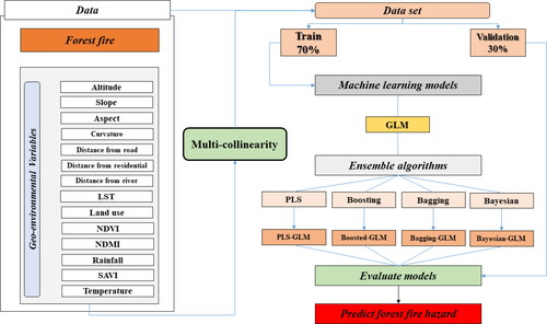
The proposed approach for modeling forest fires is comprised of several distinct steps, as depicted in Figure 3. The methodological flowchart outlines the process from start to finish, including the crucial steps of data preparation, data exploration, data splitting, application of machine learning techniques, evaluation of model performance, and finally forest fire susceptibility maps.

Figure 3. Methodological flow chart.

3.1. Multicollinearity

Multicollinearity is a problem that arises when predictor variables in machine learning (ML) models are highly correlated with each other. This can result in unreliable coefficients, reduced interpretability of the model, and decreased prediction accuracy (Alin, 2010). To mitigate these issues, it is essential to assess the strength of multicollinearity among input variables in ML models. One of the most widely used metrics for assessing multicollinearity is the variance inflation factor (VIF). VIF quantifies the increase in variance of an estimated regression coefficient due to collinearity in the predictor variables (Paul, 2006). The VIF is calculated as: (5) $$\mathrm{VIF}=1/(1-R_i^2),$$(5) where $R_i^2$ is the determination coefficient of the regression of the i^th predictor variable on all the other predictor variables. VIF values less than 1 imply no multicollinearity, while VIF values from 1 to 5 show mild multicollinearity. Moderate multicollinearity occurs when the VIF is between 5 and 10, and severe multicollinearity happens for the VIF of larger than 10. By conducting a VIF analysis, researchers can gain insights into the extent of multicollinearity among input variables and make informed decisions about which predictor variables to include or exclude from the model (Paul, 2006; Alin, 2010).

3.2. Modeling and ensemble approaches

ML-based models use artificial intelligence (AI) techniques that successfully equip machines to learn from experience without being explicitly programmed (Ardabili et al. 2019). Ensemble learning has been developed in ML to advance the robustness and accuracy of a model. Ensemble learning algorithms, such as ‘boosting’ and ‘bagging’, simplify solutions to key computational issues (Zhang and Ma, 2012). In this study, the GLM and four ensemble approaches (PLS, Boosting, Bagging and Bayesian) were employed to model the forest fire risk. For this purpose, the R software with the caret, raster, brms, mboost, and plsRglm packages were employed (Kuhn 2012, Hothorn et al. 2013, Bertrand et al. 2014, Hijmans et al. 2015, Buerkner and Buerkner 2016).

3.2.1. Generalized linear model (GLM)

GLMs are frequently used to model binary or count data as flexible generalizations of ordinary linear regression. They enable the response factors to provide error distributions except a normal distribution (McCulloch and Searle 2014). GLMs simulate the response variable by a linear model and employ the variance of each observation as a function of its predicted value (Kamata, 2001). Each output (Y) is presumed to be produced from a specific distribution. The average ($\overline{A}$) of the distribution depends on the independent variable X according to Equation (6)(6) $$F\left(Y\right)=g^{-1}\left(X_{\beta }\right)=\overline{A},$$(6) (Wolfinger and O'connell, 1993; Stroup, 2012): (6) $$F\left(Y\right)=g^{-1}\left(X_{\beta }\right)=\overline{A},$$(6) where X_β is the linear predictor as a linear integration of the unknown parameter β, F(Y) is the expected value of Y, and g is the link function. Accordingly, the variance (V) is usually a function of the average value, as shown in Equation (7)(7) $$\mathrm{Var}\mathrm{ }\left(Y\right)=V\left(\overline{A}\right)=g^{-1}\left(XB\right),$$(7) (Wolfinger and O'connell, 1993; Stroup, 2012): (7) $$\mathrm{Var}\mathrm{ }\left(Y\right)=V\left(\overline{A}\right)=g^{-1}\left(XB\right),$$(7)

This is appropriate if V contains an exponential distribution, but it may be convenient for the variance to be a function of the predicted value. B is an unknown parameter that can be successfully estimated by maximum likelihood, maximum quasi-likelihood, or Bayesian techniques (Stroup, 2012).

3.2.2. Partial least-squares PLSGLM

PLSGLM employs a complex of orthogonal latent factors (LFs) to model the response variables. The set of LFs was exported from a large number of independent variables using PLS (Marx, 1996; Ding and Gentleman 2005). It was generated by projecting the dataset onto a lower-dimensional subspace, while maximizing the covariance between the LF. This process is conducted in a way that the LFs describe most of the covariance between Y:N × M and X:N × P (Park et al. 2002). These LFs (usually called X-scores) are few (A < P). Often, they are shown by T, and because the LFs must be orthogonal, T^TT = I_A. Several algorithms have been employed for computing LFs, such as kernels and statistical modifications to PLS and nonlinear iterative PLS (Ding and Gentleman 2005).

Different algorithms, such as kernel PLS, orthogonal partial least square (OPLS), sparse partial least square (SPLS), result in distinct PLS decompositions. For all cases, T:N × A, and a matrix of X-scores is found as T = X₀R. PLS employs matrix T as an independent variable to model Y, as shown in Equation (8)(8) $${\widehat{Y}}_0={\left(T\right)}^{-1}{T}^T=T{T}^T{Y}_0\widetilde{=}T{Q}^T=X_{0}R{Q}^T={X_0\widehat{B}}_{\mathit{PLS}},$$(8) (Marx, 1996): (8) $${\widehat{Y}}_0={\left(T\right)}^{-1}{T}^T=T{T}^T{Y}_0\widetilde{=}T{Q}^T=X_{0}R{Q}^T={X_0\widehat{B}}_{\mathit{PLS}},$$(8) where A is the number of PLS components and ${{ }_{ }\widehat{B}}_{\mathit{PLS}}$ is the predicted coefficient matrix for the PLS model. This model can be extended to the GLM, as in Equation (9)(9) $$g\left(A\right)={X_0\widehat{B}}_{\mathit{PLS}-\mathit{GLM}},$$(9) (Marx, 1996): (9) $$g\left(A\right)={X_0\widehat{B}}_{\mathit{PLS}-\mathit{GLM}},$$(9) where ${\widehat{B}}_{\mathit{PLS}-\mathit{GLM}}=R_{*}{q}_{*}$ is the PLS-GLM coefficient vector, and R_∗ and q_∗:A × 1 are calculated from the PLS-GLM.

3.2.3. Boosted GLM

Variable selection can be considered as one of the main tasks in the GLM. The first step can be performed without any random effects. In boosted GLM, the variables could be added only to the last selected model, with the disadvantage that it may not be optimal. Boosted GLM is a modern method that selects the inclusion parameters. Boosting-based techniques are often used in ML communities to increase classification accuracy. In boosted GLM, random effects are simultaneously fitted to the model parameters (mstop and prune) (Bou-Hamad et al. 2017). The method starts with a minimal number of variables and gradually increases them until the end criterion is met. This component-wise approach starts with all parameters set to zero and updates them iteratively, leading to an optimized model.

3.2.4. Bagging GLM

Bagging enhances model accuracy that starts by aggregating several predictors (Breiman, 1996; Sutton, 2005). This technique works by developing a base-learning algorithm using a trial-and-error method on various training sets (Breiman, 1996). Bagging improves the stability and predictive robustness of the regression and classification models. In this study, the bagging approach was selected to weigh the presence data (fire points) and determine its importance over the absence data (non-fire points).

First, the dataset was separated into presence and absence data. Then, equal number of presence and absence data were selected by bootstrapping. Accordingly, the GLM was employed with a binomial error with the total data. The combination of bagging and GLM provides a valuable tool for modeling complex systems and predicting forest fire risk, taking into account the influence of various factors and providing a comprehensive understanding of the underlying patterns in the data.

3.2.5. Bayesian GLM

Bayesian inference is a probabilistic approach, which is built on the concept that for each quantity, there is a probability distribution that can be optimized for new data. Bayesian networks (also called belief networks) are probabilistic models that signify information in an unspecified context. Each node in the diagram shows a random variable, and the branches indicate possible dependencies between them (Tran et al. 2020). These conditional dependencies are usually assessed using probabilistic and statistical approaches. Bayesian networks merge statistics, computer science, principles of graph theory, and probability theory. They efficiently represent and calculate probability distributions in a series of random variables (Band et al. 2020). The use of Bayesian methods for the proper modeling and determination of optimal parameters has been undertaken in recent years (Ahmadi et al. 2020). In this study, the Bayesian method was combined with cumulative linear regression to estimate the risk of forest fires.

3.3. Validation and accuracy assessment

The receiver operating characteristic (ROC) is often used as an evaluation metric for binary classification models. The ROC plots the relationship between the true positive rate (sensitivity) and false positive rate (1-specificity) at various classification thresholds. The area under the curve (AUC) of the ROC plot denotes the performance of a classifier. It ranges from 0 to 1 with the AUC of closer to unity indicates a better model performance. AUC is a useful metric as it summarizes the performance of the classifier across all thresholds and provides an overall measure of its discriminative ability (Peres and Cancelliere 2014).

Sensitivity, Specificity, PPV, and NPV are important metrics in evaluating binary classification models. Sensitivity (also known as the true positive rate) measures the proportion of positive cases that are correctly identified as positive (equation 10(10) $$\mathrm{Sensitivity}=\frac{\text{True positive}}{\text{True positive}+\text{False negative}},\mathrm{ }$$(10) ). Specificity (also known as the true negative rate) measures the proportion of negative cases that are correctly identified as negative (equation 11(11) $$\mathrm{Specificity}=\frac{\text{True negative}}{\text{True negative}+\text{False positive}},\mathrm{ }$$(11) ). Positive predictive value (PPV) and Negative Predictive Value (NPV) provide a measure of the precision of the classifier's positive and negative predictions, respectively. PPV is the proportion of positive predictions that are actually positive (equation 12(12) $$\mathrm{PPV}=\frac{\text{True negative}}{\text{False positive}+\text{True positive}},\mathrm{ }$$(12) ), while NPV is the proportion of negative predictions that are actually negative (equation 13(13) $$\mathrm{NPV}=\frac{\text{True positive}}{\text{True positive}+\text{False negative}}.\mathrm{ }$$(13) ). These metrics are essential in understanding the strengths and limitations of a classification model and provide valuable insights into its performance (Peres and Cancelliere 2014; Yonelinas, 1994). (10) $$\mathrm{Sensitivity}=\frac{\text{True positive}}{\text{True positive}+\text{False negative}},\mathrm{ }$$(10) (11) $$\mathrm{Specificity}=\frac{\text{True negative}}{\text{True negative}+\text{False positive}},\mathrm{ }$$(11) (12) $$\mathrm{PPV}=\frac{\text{True negative}}{\text{False positive}+\text{True positive}},\mathrm{ }$$(12) (13) $$\mathrm{NPV}=\frac{\text{True positive}}{\text{True positive}+\text{False negative}}.\mathrm{ }$$(13)

4. Results and discussion

Table 2 presents the VIF and tolerance values for the 14 independent variables utilized for modeling forest fires. The results show that all 14 variables have a VIF below 5. NDVI has the highest VIF value of 4.23 and Aspect has the lowest VIF value of 1.10.

Table 2. Result of the multi-collinearity analysis.

Row	Variables	VIF	Tolerance
1	Altitude	3.08	0.32
2	Slope	1.51	0.66
3	Aspect	1.1	0.91
4	Curvature	1.19	0.84
5	Distance from river	1.84	0.54
6	Distance from road	1.54	0.65
7	Distance from residential	2.12	0.47
8	Land use	1.9	0.53
9	LST	3.26	0.31
10	NDMI	3.95	0.25
11	NDVI	4.23	0.24
12	SAVI	3.06	0.33
13	Annual rainfall	1.41	0.71
14	Annual temperature	2.48	0.40

For both training and testing phases, the sensitivity, specificity, NPV, PPV, and area under curve (AUC) metrics of five models (namely GLM, PLS-GLM, Boosted-GLM, Bagging-GLM, and Bayesian-GLM) are shown in Table 3. The AUC values from these models during the testing phase are presented in Figure 4. In the testing phase, the AUC values of the GLM, PLS-GLM, Boosted-GLM, Bagging-GLM, and Bayesian-GLM were 0.79, 0.75, 0.81, 0.84, and 0.85, respectively.

Figure 4. ROC curve analysis for forest fire susceptibility models using the validation dataset (The vertical axis is the true positive fraction (TPF) value and the horizontal axis represents the false positive fraction (FPF) value.).

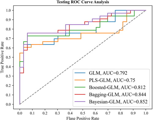
Table 3. Predictive capability of forest fire models using training and testing datasets.

Model	Stage	Evaluation parameter
		Sensivity	Specifity	NPV	PPV	AUC
GLM	Training	0.80	0.77	0.78	0.79	0.85
	Testing	0.64	0.88	0.84	0.71	0.79
PLSGLM	Training	0.75	0.71	0.72	0.74	0.81
	Testing	0.63	0.85	0.81	0.70	0.75
Boosted GLM	Training	0.80	0.79	0.79	0.80	0.87
	Testing	0.67	0.96	0.95	0.74	0.81
Bagging GLM	Training	0.80	0.79	0.79	0.80	0.86
	Testing	0.73	0.94	0.92	0.77	0.84
Bayesian GLM	Training	0.83	0.81	0.79	0.80	0.88
	Testing	0.73	0.95	0.93	0.78	0.85

The evaluation metrics indicated that the Boosting, Bagging and Bayesian ensemble methods improved the efficiency of the GLM in predicting forest fires. Similarly, other studies (e.g. Xie and Peng 2019; Naghibi et al. 2020; Sanjaya and Puspitasari 2020) showed that ensemble models tend to be more accurate than individual models in forest fire hazard modeling. This finding is consistent with the previous studies that showed the superiority of ensemble models in predicting floods (Hosseini et al. 2020), landslide and debris flow (Pal et al. 2022), erosion (Band et al. 2020) and multi-hazard (Saha et al. 2021).

The Bayesian-GLM had the highest efficiency compared to the other three ensemble models. The Bayesian-GLM has several advantages in modeling natural hazards. First, it incorporates prior knowledge and uncertainties into the model parameters, resulting in predictions that are both accurate and reliable. This is especially crucial in the context of natural hazards, where data are often limited and uncertain. By aggregating the outputs of ensemble models, the Bayesian-GLM can produce predictions that are more accurate and reliable. This has a significant impact on the management and mitigation of natural hazards. Additionally, the Bayesian-GLM allows for the assessment of model uncertainty, which can be particularly valuable for decision-making in high-stakes and high-uncertain situations (Zhao at al. 2006; de los Campos and Pérez-Rodríguez 2014; Hosseini et al. 2020).

Using the Jenk's natural breaks model in ArcGIS 10.5 (Jenks, 1967; McMaster, 1997), the forest fire susceptibility map of the Chalus watershed was classified into very high, high, moderate, low, and very low. Figure 5 displays the classified forest fire susceptibility map based on GLM and four hybrid models (PLS-GLM, boosted-GLM, bagging-GLM, and Bayesian-GLM). The spatial resolution of generated fire susceptibility maps is 30 m. Table 4 lists the area (km²) and percentage of each forest fire susceptibility class.

Figure 5. Forest fire susceptibility using five algorithms: a) GLM, b) PLS-GLM, c) Boosted-GLM, d) Bagging-GLM, and e) Bayesian-GLM.

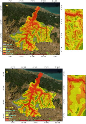
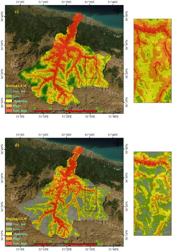
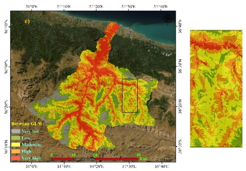
Table 4. Forest fire susceptibility class areas.

Model	Area	Susceptibility Class
		Very low	Low	Moderate	High	Very high
GLM	km^2	104.2	261.14	460.35	505.56	300.26
	%	6.39	26.01	28.22	30.99	18.4
PLSGLM	km^2	111.2	262.39	452.45	471.78	333.69
	%	6.82	16.08	27.73	28.92	20.45
Boosted GLM	km^2	99.77	245.51	435.68	494.39	356.16
	%	6.12	15.05	26.70	30.30	21.83
Bagging GLM	km^2	392.3	365.02	309.77	296.78	267.64
	%	24.05	22.37	18.99	18.19	16.40
Bayesian GLM	km^2	105.82	273.87	472.78	480.89	298.15
	%	6.49	16.79	28.98	29.48	18.27

According to Table 4, the output of GLM owns about ∼6.4% at very low class of 104.2 km²_, 26% at low class of 261.14 km², 28.22% at moderate class of 460.35 km², 31% at high class of 505.56 km² and 18.4% at very high class of 300.26 km². However, the Bayesian-GLM owns about 6.49% at very low class of 105.82 km²_, 16.8% at low class of 273.87 km², 28.98% at moderate class of 472.78 km², 29.48% at high class of 480.89 km² and 18.27% at very high class of 298.15 km².

The importance of input variables was obtained based on the Gini index (Sandri and Zuccolotto 2008). It is a commonly used index for determining the importance of inputs in machine learning models. This index measures the reduction in impurity (incorrect predictions) in a binary split of the data based on a particular variable. The Gini importance score is calculated as the weighted average of the decrease in impurity for each split, where the weight is proportional to the number of samples in the node. This score can be used to rank input variables based on their contribution to the outputs (Sandri and Zuccolotto, 2008; Pourghasemi et al. 2020). Table 5 displays the importance values for each variable. The highest importance value is for ‘Altitude’ with a score of 100 and the lowest is for ‘Aspect’ with a score of 3.11. Variables with moderate importance are ‘Distance from river’, ‘Distance from road’, ‘Rainfall’, ‘LST’, and ‘Temperature’ with scores of 60.97, 69.10, 77.26, 42.39, and 60.65, respectively. The partial dependence plots of forest fires for these four variables are depicted in Figure 6.

Figure 6. Partial dependence plots showcasing the influence of four explanatory variables on forest fire susceptibility; a) altitude and rainfall, b) distance from road and distance from river.

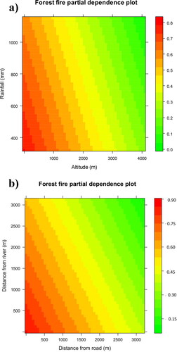
Table 5. Results of determination of importance value.

Variable	Importance value
Altitude	100
Slope	19.78
Aspect	3.11
Curvature	36.95
Distance from river	60.97
Distance from road	69.10
Distance from residential area	17.33
Land use	4.51
LST	42.39
NDMI	16.84
NDVI	22.62
SAVI	22.64
Rainfall	77.26
Temperature	60.65

This study investigated the impact of various factors on fire risk in the Chalus Rood basin. We found that elevation, rainfall, distance from the road, distance from the river, and temperature had the most significant influence on fire risk. The results showed that lowlands, which are often nearby residential areas, are more susceptible to forest fire hazards compared to high-altitude regions. This finding is in agreement with previous studies (e.g. Flannigan and Haar, 1986;; Milanović et al. 2020) that identified elevation as an important variable in determining fire hazards.

This study also indicated that the risk of forest fires increases with decreasing rainfall and increasing temperature. These atmospheric factors have a major impact on the region’s humidity and have a dominant control on the ignition and spread of fires. Moist conditions from high amounts of rainfall reduce the risk of fires, while low rainfall and drought conditions increase the risk by accumulating dry fuels, which can cause fires to spread rapidly (Abram et al. 2021; Dhar et al. 2023). Temperature also plays a crucial role in forest fire susceptibility. Higher temperatures can increase the evaporation rate of moisture in the fuels, leading to an increased risk of fire. Additionally, high temperatures can cause an increase in atmospheric instability, which leads to the formation of thunderstorms, and lightning strikes can ignite fires in the forests (de Santana et al. 2021; Akıncı and Akıncı, 2023). Eskandari et al. (2020) explored the relationship between climatic factors and the incidence of fires in northeastern Iran. They found a positive correlation between air temperature and fire risk. Their results also indicated a negative relationship between rainfall and fire.

Moreover, our study found that the distance from roads is another crucial factor affecting the risk of forest fires in the Chalus Rood basin. This variable reflects human impacts on fire occurrences and plays an important role in spreading fires in the surrounding region. The road map of the study area highlights that areas close to roads are at a high risk of forest fire. The roads and residential areas in the Chalus Rood watershed positively contribute to the occurrence of fires as tourists and/or residents can cause fires. These results match with those of Jaiswal et al. (2002), Erten et al. (2004), Bui et al. (2017), and Pandey and Ghosh (2018) that showed the distance from roads is the major cause of forest fires by humans.

5. Conclusion

In this study, fire risk was investigated using four ensemble algorithms on the GLM model in the Chalus Rood basin in Iran, and a fire hazard model were developed using these algorithms. All ensemble algorithms, except the PLS algorithm, increased the efficiency of the GLM model, and the Bayesian algorithm was the most efficient algorithm for improving the performance of the GLM model. The features of the study area, including topographic factors affecting the occurrence of fire, accuracy and type of layers of independent variables to model the risk of fire, accuracy of recorded points and ranges of past fires, and type of prediction algorithms used, affected the overall classification accuracy of this study. Because the impact of most fires in the Chalus Rood basin can be increased by increasing the effective human variables, the accuracy and precision of hazard maps can be increased. The high accuracy of the fire prediction models in this study makes them useful for creating fire probability maps in other northern regions of Iran. These maps can help manage the risk of forest fires, prevent them, and quickly extinguish any that occur. Based on these maps, facilities for dealing with fires in high-risk areas can be established, such as watchtowers and water tanks in inaccessible areas, wireless sensor networks for early detection, and rescue bases before the fire season. To further prevent and reduce fire damage, it is important to raise awareness, educate the local population, and establish fire pits and barriers. One of the limitations of this study is the inaccessibility of a few influential climate variables such as wind speed, wind direction, and humidity. Thus, we could not use them in mapping forest fire susceptibility. It is recommended that future studies utilize these climate variables in modeling forest fire susceptibility maps. Additionally, it is suggested to use other forest fire mapping approaches (e.g. deep learning techniques and hybrid machine learning models) and compare their results with the findings in this study.

Acknowledgment

We would like to acknowledge the anonymous reviewers.

Disclosure statement

No potential conflict of interest was reported by the author(s).

Data availability statement

Due to the nature of this research, participants of this study did not agree for their data to be shared publicly, so supporting data is not available.

References

- Abdo HG, Almohamad H, Al Dughairi AA, Al-Mutiry M. 2022. GIS-based frequency ratio and analytic hierarchy process for forest fire susceptibility mapping in the western region of Syria. Sustainability. 14(8):4668.
- Abedi Gheshlaghi H,Feizizadeh B,Blaschke T,Lakes T,Tajbar S. 2021. Forest fire susceptibility modeling using hybrid approaches. Trans GIS. 25(1):311–333.
- Abram NJ,Henley BJ,Sen Gupta A,Lippmann TJR,Clarke H,Dowdy AJ,Sharples JJ,Nolan RH,Zhang T,Wooster MJ, et al. 2021. Connections of climate change and variability to large and extreme forest fires in southeast Australia. Commun Earth Environ. 2(1).
- Achu AL, Thomas J, Aju CD, Gopinath G, Kumar S, Reghunath R. 2021. Machine-learning modelling of fire susceptibility in a forest-agriculture mosaic landscape of southern India. Ecol Inf. 64:101348.
- Adab H,Kanniah KD,Solaimani K. 2013. Modeling forest fire risk in the northeast of Iran using remote sensing and GIS techniques. Nat Hazards. 65(3):1723–1743.
- Agranat V, Perminov V. 2020. Mathematical modeling of wildland fire initiation and spread. Environ Model Softw. 125:104640.
- Ahmadi K,Kalantar B,Saeidi V,Harandi EKG,Janizadeh S,Ueda N. 2020. Comparison of machine learning methods for mapping the stand characteristics of temperate forests using multi-spectral sentinel-2 data. Remote Sens. 12(18):3019.
- Ahmed MR, Hassan QK, Abdollahi M, Gupta A. 2020. Processing of near real time land surface temperature and its application in forecasting forest fire danger conditions. Sensors. 20(4):984.
- Akıncı HA, Akıncı H. 2023. Machine learning based forest fire susceptibility assessment of Manavgat district (Antalya), Turkey. Earth Sci Inform. 16(1):397–414.
- Alin A. 2010. Multicollinearity. WIREs Comp Stat. 2(3):370–374.
- Ardabili S, Mosavi A, Dehghani M, Várkonyi-Kóczy AR. 2019. Deep learning and machine learning in hydrological processes climate change and earth systems a systematic review. In International conference on global research and education. Cham: Springer; p. 52–62.
- Band SS, Janizadeh S, Saha S, Mukherjee K, Bozchaloei SK, Cerdà A, Shokri M, Mosavi A. 2020. Evaluating the efficiency of different regression, decision tree, and bayesian machine learning algorithms in spatial piping erosion susceptibility using ALOS/PALSAR Data. Land. 9(10):346.
- Bera B, Shit PK, Sengupta N, Saha S, Bhattacharjee S. 2022. Forest fire susceptibility prediction using machine learning models with resampling algorithms, Northern part of Eastern Ghat Mountain range (India). Geocarto Int. 37(26):11756–11781.
- Bera B, Shit PK, Sengupta N, Saha S, Bhattacharjee S. 2022. Susceptibility of deforestation hotspots in Terai-Dooars belt of Himalayan Foothills: a comparative analysis of VIKOR and TOPSIS models. J King Saud Univ–Comput Inform Sci. 34(10):8794–8806.
- Bertrand F, Meyer N, Bertrand MF. 2014. Package ‘plsRglm.
- Bou-Hamad I, Anouze AL, Larocque D. 2017. An integrated approach of data envelopment analysis and boosted generalized linear mixed models for efficiency assessment. Ann Oper Res. 253(1):77–95.
- Breiman L. 1996. Bagging predictors. Mach Learn. 24(2):123–140.
- Brillinger DR, Preisler HK, Benoit JW. 2003. Risk assessment: a forest fire example. Lecture notes–monograph series. 1:177–196.
- Buerkner PC, Buerkner MPC. 2016. Package ‘brms’. https://mran.microsoft.com/snapshot/2016-12-17/web/packages/brms/brms.pdf
- Bui DT, Bui QT, Nguyen QP, Pradhan B, Nampak H, Trinh PT. 2017. A hybrid artificial intelligence approach using GIS-based neural-fuzzy inference system and particle swarm optimization for forest fire susceptibility modeling at a tropical area. Agric Meteorol. 233:32–44.
- Bui DT, Le K-TT, Nguyen VC, Le HD, Revhaug I. 2016. Tropical forest fire susceptibility mapping at the cat Ba National Park Area, Hai Phong City, Vietnam, Using GIS-based kernel logistic regression. Remote Sens. 8(4):347.
- Carvalho FJ,Santana DGd,Araújo LBd. 2018. Why analyze germination experiments using Generalized Linear Models?. J Seed Sci. 40(3):281–287.
- Cheret V, Denux JP. 2011. Analysis of MODIS NDVI time series to calculate indicators of Mediterranean forest fire susceptibility. GIScience & Remote Sensing. 48(2):171–194.
- Chew YJ, Ooi SY, Pang YH, Wong KS. 2022. A Review of forest fire combating efforts, challenges and future directions in Peninsular Malaysia, Sabah, and Sarawak. Forests. 13(9):1405.
- Chicas SD, Østergaard Nielsen J. 2022. Who are the actors and what are the factors that are used in models to map forest fire susceptibility? A systematic review. Nat Hazards. 114(3):2417–2434.
- Chuvieco E, Cocero D, Riaño D, Martin P, Martı́nez-Vega J, de la Riva J, Pérez F., 2004. Combining NDVI and surface temperature for the estimation of live fuel moisture content in forest fire danger rating. Remote Sens Environ. 92(3):322–331.
- Collin A, Bernardin D, Sero-Guillaume O. 2011. A physical-based cellular automaton model for forest-fire propagation. Combust Sci Technol. 183(4):347–369.
- Das J, Mahato S, Joshi PK, Liou YA. 2023. Forest fire susceptibility zonation in Eastern India using statistical and weighted modelling approaches. Remote Sensing. 15(5):1340.
- de los Campos G, Pérez-Rodríguez P. 2014. Bayesian generalized linear regression. R Package Version1.0.4. http://CRAN.R-project.org/package=BGLR.
- de Santana RO, Delgado RC, Schiavetti A. 2021. Modeling susceptibility to forest fires in the Central Corridor of the Atlantic Forest using the frequency ratio method. J Environ Manage. 296:113343.
- Dhar T,Bhatta B,Aravindan S. 2023. Forest fire occurrence, distribution and risk mapping using geoinformation technology: A case study in the sub-tropical forest of the Meghalaya, India. Remote Sens. Appl: Soc. Environ. 29:100883.
- Digavinti J, Manikiam B. 2021. Satellite monitoring of forest fire impact and regeneration using NDVI and LST. J Appl Rem Sens. 15(04):042412–042412.
- Ding B, Gentleman R. 2005. Classification using generalized partial least squares. J Comput and Graph Stat. 14(2):280–298.
- Eastaugh CS, Hasenauer H. 2014. Deriving forest fire ignition risk with biogeochemical process modelling. Environ Model Softw. 55:132–142.
- Erten E, Kurgun V, Musaoglu N. 2004. Forest fire risk zone mapping from satellite imagery and GIS. a case study. In XXth Congress of the international society for photogrammetry and remote sensing congress, Istanbul, Turkey; p. 222–230.
- Eskandari S, Amiri M, Sãdhasivam N, Pourghasemi HR. 2020. Comparison of new individual and hybrid machine learning algorithms for modeling and mapping fire hazard: a supplementary analysis of fire hazard in different counties of Golestan Province in Iran. Nat Hazards. 104(1):305–327.
- Flannigan MD, Haar TV. 1986. Forest fire monitoring using NOAA satellite AVHRR. Can J for Res. 16(5):975–982.
- Gigović L, Pourghasemi HR, Drobnjak S, Bai S. 2019. Testing a new ensemble model based on SVM and random forest in forest fire susceptibility assessment and its mapping in Serbia’s Tara National Park. Forests. 10(5):408.
- Gonzalez-Olabarria JR,Brotons L,Gritten D,Tudela A,Teres JA. 2012. Identifying location and causality of fire ignition hotspots in a Mediterranean region. Int J Wildland Fire. 21(7):905–914.
- Hijmans RJ, Van Etten J, Cheng J, Mattiuzzi M, Sumner M, Greenberg JA, Lamigueiro OP, Bevan A, Racine EB, Shortridge A, et al. 2015. Package ‘raster’. R Package. 734:473.
- Hong H,Tsangaratos P,Ilia I,Liu J,Zhu A-X,Xu C. 2018. Applying genetic algorithms to set the optimal combination of forest fire related variables and model forest fire susceptibility based on data mining models. The case of Dayu County, China. Sci Total Environ. 630:1044–1056. 10.1016/j.scitotenv.2018.02.278. 29554726
- Hosseini FS, Choubin B, Mosavi A, Nabipour N, Shamshirband S, Darabi H, Haghighi AT. 2020. Flash-flood hazard assessment using ensembles and Bayesian-based machine learning models: application of the simulated annealing feature selection method. Sci Total Environ. 711:135161.
- Hothorn T, Buehlmann P, Kneib T, Schmid M, Hofner B, Sobotka F, Scheipl F. 2013. Package ‘mboost.
- Huebner K, Lindo Z, Lechowicz MJ. 2012. Post-fire succession of collembolan communities in a northern hardwood forest. Eur J Soil Biol. 48:59–65.
- Huesca M, Litago J, Palacios-Orueta A, Montes F, Sebastián-López A, Escribano P. 2009. Assessment of forest fire seasonality using MODIS fire potential: a time series approach. Agric Meteorol. 149(11):1946–1955.
- Jaafari A,Zenner EK,Panahi M,Shahabi H. 2019. Hybrid artificial intelligence models based on a neuro-fuzzy system and metaheuristic optimization algorithms for spatial prediction of wildfire probability. Agric For Meteorol. 266–267:198–207.
- Jain P, Coogan SC, Subramanian SG, Crowley M, Taylor S, Flannigan MD. 2020. A review of machine learning applications in wildfire science and management. Environ Rev. 28(4):478–505.
- Jaiswal RK, Mukherjee S, Raju KD, Saxena R. 2002. Forest fire risk zone mapping from satellite imagery and GIS. Int J Appl Earth Obs Geoinf. 4(1):1–10.
- Junaidi SN, Khalid N, Othman AN, Hamid JRA, Saad NM. 2021. Analysis of the Relationship between Forest Fire and Land Surface Temperature using Landsat 8 OLI/TIRS Imagery. In IOP Conf Ser: Earth Environ Sci. 767(1):012005. May(IOP Publishing.
- Kalantar B, Ueda N, Idrees MO, Janizadeh S, Ahmadi K, Shabani F. 2020. Forest fire susceptibility prediction based on machine learning models with resampling algorithms on remote sensing data. Remote Sens. 12(22):3682.
- Kamata A. 2001. Item analysis by the hierarchical generalized linear model. J Educ Meas. 38(1):79–93.
- Kant Sharma L, Kanga S, Singh Nathawat M, Sinha S, Chandra Pandey P. 2012. Fuzzy AHP for forest fire risk modeling. Dis Preven Manage: Int J. 21(2):160–171.
- Kuhn M. 2012. The caret package. R Foundation for Statistical Computing, Vienna, Austria. https://cran.r-project.org/package=caret.
- Kwak H, Lee WK, Saborowski J, Lee SY, Won MS, Koo KS, Lee MB, Kim SN. 2012. Estimating the spatial pattern of human-caused forest fires using a generalized linear mixed model with spatial autocorrelation in South Korea. Int J Geograph Inform Sci. 26(9):1589–1602.
- Lattimer BY, Hodges JL, Lattimer AM. 2020. Using machine learning in physics-based simulation of fire. Fire Saf J. 114:102991.
- Mabdeh AN, Al-Fugara AK, Khedher KM, Mabdeh M, Al-Shabeeb AR, Al-Adamat R. 2022. Forest fire susceptibility assessment and mapping using support vector regression and adaptive Neuro-Fuzzy inference system-based evolutionary algorithms. Sustainability. 14(15):9446.
- Maffei C,Alfieri S,Menenti M. 2018. Relating Spatiotemporal Patterns of Forest Fires Burned Area and Duration to Diurnal Land Surface Temperature Anomalies. Remote Sens. 10(11):1777.
- Marx BD. 1996. Iteratively reweighted partial least squares estimation for generalized linear regression. Technometrics. 38(4):374–381.
- McCulloch CE, Searle SR. 2004. Generalized, linear, and mixed models. Hoboken, NJ: John Wiley & Sons.
- McMaster R. 1997. In Memoriam: George F. Jenks (1916-1996). Cartogr Geogr Inf Sci. 24(1):56–59.
- Milanović S, Marković N, Pamučar D, Gigović L, Kostić P, Milanović SD. 2020. Forest fire probability mapping in eastern Serbia: logistic regression versus random forest method. Forests. 12(1):5.
- Mohajane M, Costache R, Karimi F, Pham QB, Essahlaoui A, Nguyen H, Laneve G, Oudija F. 2021. Application of remote sensing and machine learning algorithms for forest fire mapping in a Mediterranean area. Ecol Indic. 129:107869.
- Naghibi SA, Hashemi H, Berndtsson R, Lee S. 2020. Application of extreme gradient boosting and parallel random forest algorithms for assessing groundwater spring potential using DEM-derived factors. J Hydrol. 589:125197.
- Nuthammachot N, Stratoulias D. 2021. Multi-criteria decision analysis for forest fire risk assessment by coupling AHP and GIS: method and case study. Environ Dev Sustain. 23(12):17443–17458.
- Pal SC,Chakrabortty R,Saha A,Bozchaloei SK,Pham QB,Linh NTT,Anh DT,Janizadeh S,Ahmadi K. 2022. Evaluation of debris flow and landslide hazards using ensemble framework of Bayesian- and tree-based models. Bull Eng Geol Environ. 81(1).
- Pandey K, Ghosh SK. 2018. Modeling of parameters for forest fire risk zone mapping. Int Arch Photogramm Remote Sens Spatial Inf Sci. XLII-5:299–304.
- Pang Y, Li Y, Feng Z, Feng Z, Zhao Z, Chen S, Zhang H. 2022. Forest Fire Occurrence Prediction in China Based on Machine Learning Methods. Remote Sensing. 14(21):5546.
- Pham BT, Jaafari A, Avand M, Al-Ansari N, Dinh Du T, Yen HPH, Phong TV, Nguyen DH, Le HV, Mafi-Gholami D, et al. 2020. Performance evaluation of machine learning methods for forest fire modeling and prediction. Symmetry. 12(6):1022.
- Park PJ, Tian L, Kohane IS. 2002. Linking gene expression data with patient survival times using partial least squares. Bioinformatics. 18(suppl_1):S120–S127.
- Paul RK. 2006. Multicollinearity: causes, effects and remedies. IASRI, New Delhi. 1(1):58–65.
- Peres DJ, Cancelliere A. 2014. Derivation and evaluation of landslide-triggering thresholds by a Monte Carlo approach. Hydrol Earth Syst Sci. 18(12):4913–4931.
- Pourghasemi HR. 2016. GIS-based forest fire susceptibility mapping in Iran: a comparison between evidential belief function and binary logistic regression models. Scand J Res. 31(1):80–98.
- Pourghasemi HR, Kariminejad N, Amiri M, Edalat M, Zarafshar M, Blaschke T, Cerda A. 2020. Assessing and mapping multi-hazard risk susceptibility using a machine learning technique. Sci Rep. 10(1):3203.
- Pourghasemi HR, Gayen A, Lasaponara R, Tiefenbacher JP. 2020. Application of learning vector quantization and different machine learning techniques to assessing forest fire influence factors and spatial modelling. Environ Res. 184:109321.
- Pourtaghi ZS, Pourghasemi HR, Rossi M. 2015. Forest fire susceptibility mapping in the Minudasht forests, Golestan province, Iran. Environ Earth Sci. 73(4):1515–1533.
- Prasad AM, Iverson LR, Liaw A. 2006. Newer classification and regression tree techniques: bagging and random forests for ecological prediction. Ecosystems. 9(2):181–199.
- Reinhardt ED,Keane RE,Brown JK. 2001. Modeling fire effects. Int J Wildland Fire. 10(4):373.
- Reyes-Bueno F, Loján-Córdova J. 2022. Assessment of three machine learning techniques with open-access geographic data for forest fire susceptibility monitoring—evidence from Southern Ecuador. Forests. 13(3):474.
- Ríos-Pena L,Kneib T,Cadarso-Suárez C,Marey-Pérez M. 2017. Predicting the occurrence of wildfires with binary structured additive regression models. J Environ Manage. 187:154–165.
- Rubí JN, de Carvalho PH, Gondim PR. 2023. Application of machine learning models in the behavioral study of forest fires in the Brazilian Federal District region. Eng Appl Artif Intell. 118:105649.
- Saha A,Pal SC,Santosh M,Janizadeh S,Chowdhuri I,Norouzi A,Roy P,Chakrabortty R. 2021. Modelling multi-hazard threats to cultural heritage sites and environmental sustainability: The present and future scenarios. J Cleaner Prod. 320:128713.
- Saha S, Bera B, Kumar Shit P, Bhattacharjee S, Sengupta N. 2023. Prediction of forest fire susceptibility applying machine and deep learning algorithms for conservation priorities of forest resources. Rem Sens Appl: Soc Environ. 29:100917.
- Sandri M, Zuccolotto P. 2008. A bias correction algorithm for the Gini variable importance measure in classification trees. J Comput Graph Stat. 17(3):611–628.
- Sanjaya R, Puspitasari D. 2018. August. Noise Reduction through Bagging on Neural Network Algorithm for Forest Fire Estimates. In 2018 6th International Conference on Cyber and IT Service Management (CITSM) (pp. 1–5). IEEE.
- Setiawan I,Mahmud AR,Mansor S,Mohamed Shariff AR,Nuruddin AA. 2004. GIS‐grid‐based and multi‐criteria analysis for identifying and mapping peat swamp forest fire hazard in Pahang, Malaysia. Disaster Prev and Management. 13(5):379–386.
- Shahfahad T, Das T, Naikoo MW, Rihan M, Rahman A. 2022. Forest fire susceptibility mapping by integrating remote sensing and machine learning algorithms. Adv Rem Sens Forest Monitoring. 181–195.
- Shao Y, Feng Z, Cao M, Wang W, Sun L, Yang X, Ma T, Guo Z, Fahad S, Liu X, et al. 2023. An ensemble model for forest fire occurrence mapping in China. Forests. 14(4):704.
- Stroup WW. 2012. Generalized linear mixed models: modern concepts, methods and applications. Boca Raton, FL: CRC press.
- Sutton CD. 2005. Classification and regression trees, bagging, and boosting. In: Dey DK, Rao CR, editor. Handbook of statistics Amsterdam, Netherlands: Elsevier; p. 303–329.
- Taloor AK, Manhas DS, Kothyari GC. 2021. Retrieval of land surface temperature, normalized difference moisture index, normalized difference water index of the Ravi basin using Landsat data. Appl Comput Geosci. 9:100051.
- Talukdar S, Das T, Naikoo MW, Rihan M, Rahman A. 2022. Forest fire susceptibility mapping by integrating remote sensing and machine learning algorithms. Adv Rem Sens Forest Monitor. 2022:179–195.
- Tang X, Machimura T, Li J, Liu W, Hong H. 2020. A novel optimized repeatedly random undersampling for selecting negative samples: a case study in an SVM-based forest fire susceptibility assessment. J Environ Manage. 271:111014.
- Tariq A, Shu H, Siddiqui S, Mousa BG, Munir I, Nasri A, Waqas H, Lu L, Baqa MF. 2021. Forest fire monitoring using spatial-statistical and Geo-spatial analysis of factors determining forest fire in Margalla Hills, Islamabad, Pakistan. Geomatics Nat Hazards Risk. 12(1):1212–1233.
- Tehrany MS, Jones S, Shabani F, Martínez-Álvarez F, Bui DT. 2019. A novel ensemble modeling approach for the spatial prediction of tropical forest fire susceptibility using LogitBoost machine learning classifier and multi-source geospatial data. Theor Appl Climatol. 137(1-2):637–653.
- Tien Bui D,Hoang N-D,Samui P. 2019. Spatial pattern analysis and prediction of forest fire using new machine learning approach of Multivariate Adaptive Regression Splines and Differential Flower Pollination optimization: A case study at Lao Cai province (Viet Nam). J Environ Manage. 237:476–487.
- Tomar JS, Kranjčić N, Đurin B, Kanga S, Singh SK. 2021. Forest fire hazards vulnerability and risk assessment in Sirmaur district forest of Himachal Pradesh (India): a geospatial approach. IJGI. 10(7):447.
- Tran MN, Nguyen N, Nott D, Kohn R. 2020. Bayesian deep net GLM and GLMM. J Comput Graph Stat. 29(1):97–113.
- Vargas-Cuentas NI, Roman-Gonzalez A. 2021. Satellite-based analysis of forest fires in the bolivian chiquitania and amazon region: case 2019. IEEE Aerosp Electron Syst Mag. 36(2):38–54.
- Wolfinger R, O'connell M. 1993. Generalized linear mixed models a pseudo-likelihood approach. J Stat Comput Simul. 48(3-4):233–243.
- Xie Y, Peng M. 2019. Forest fire forecasting using ensemble learning approaches. Neural Comput Appl. 31(9):4541–4550.
- Yaakob R, Mustapha N, Nuruddin AAB, Sitanggang IS. 2011. Modeling forest fires risk using spatial decision tree. In 2011 3rd Conference on Data Mining and Optimization (DMO). Piscataway, NJ: IEEE; p. 103–107.
- Yonelinas AP. 1994. Receiver-operating characteristics in recognition memory: evidence for a dual-process model. J Exp Psychol Learn Memory Cogn. 20(6):1341–1354.
- Zhang, C. and Ma, Y. eds 2012. Ensemble machine learning: methods and applications. New York, NY: Springer Science & Business Media.
- Zheng Z, Huang W, Li S, Zeng Y. 2017. Forest fire spread simulating model using cellular automaton with extreme learning machine. Ecol Modell. 348:33–43.
- Zhao Y, Staudenmayer J, Coull BA, Wand MP. 2006. General design Bayesian generalized linear mixed models. Statist Sci. 21(1):35–51.