A LightGBM-based landslide susceptibility model considering the uncertainty of non-landslide samples

Abstract

The quality of samples is crucial in constructing a data-driven landslide susceptibility model. This article aims to construct a data-driven landslide susceptibility model that takes into account the selection of non-landslide samples. First, 21 conditioning factors are selected, including four types of topography and landform, geological conditions, environmental conditions, and human activities. Grid units with 30 m resolution are established by combining 942 historical landslide events in study area. Second, non-landslide samples are selected using both the traditional method and the information quantity method. Two landslide susceptibility models are established using the Bayesian optimization-LightGBM model. The accuracy of the model is evaluated by significance test and the area under curve (AUC). Finally, the SHAP algorithm is used to analyse the internal mechanism of the model’s decision-making. Based on the information quantity method, the LightGBM model identifies very high-high susceptibility areas that account for 77.92% of the total number of landslides. Additionally, the AUC of test set and the AUC of training set are 23.2% and 17.1% higher, respectively, compared to the traditional model. The selection of different sample data, whether landslide or non-landslide, impacts the factor rank, model accuracy, and the interal decision-making mechanism of the model. This finding provides valuable for the selection of sample data in the binary classification model.

Keywords:

• Information quantity method
• Light Gradient Boosting Machine (LightGBM)
• Bayesian optimization
• box plot diagram
• SHapley Additive exPlanation (SHAP)

1. Introduction

Landslide is a natural geological disaster that occurs worldwide, characterized by a wide impact, sudden occurrence, and multiple incidents, posing a significant threat to human life and property (Wang, Sun, et al. 2020; Wang, Feng, et al. 2020). According to records, landslides have caused an average of 4300 deaths annually worldwide (Brenning 2012). China, with its complex and diverse topography and vast mountainous area, is one of the countries most severely affected by landslide disasters. In 2021, a total of 4772 geological disasters occurred in China, resulting in 80 deaths, 11 missing persons, and economic losses of 3.2 billion yuan. Among them, 2335 landslides, accounting for 48.93% of the annual total geological disasters, caused severe economic losses, according to a geological disaster bulletin. To study the degree of landslide occurrence based on a local geological environment assessment, landslide susceptibility mapping (LSM) (Zêzere et al. 2017; D. Sun et al. 2022) is a method used to analyse spatial distribution characteristics which is of great significance for landslide disaster warning and prediction, monitoring and management, and urban planning and treatment (Hong et al. 2016).

With the rapid development of artificial intelligence technology, machine learning algorithms have been widely applied in the field of geological disaster warning. Common machine learning algorithms include logistic regression (LR) (Lombardo and Mai 2018), neural network (Zhang et al. 2022), random forest (RF) (Taalab et al. 2018; Wang et al. 2021), support vector machine (SVM) (Wang and Brenning 2021), decision tree (Wu et al. 2020), natural gradient boosting (NGBoost) (Kavzoglu and Teke 2022), and gradient boosting algorithms (Bentéjac et al. 2021; Natekin and Knoll 2013). However, LR may not be effective in addressing issues related to nonlinearity and low accuracy. Neural network often requires tuning a large number of parameters and long learning times. RF and SVM can be computationally expensive due to their algorithm complexity. Decision trees are susceptible to overfitting. The NGBoost and the Gradient Boosting Algorithms have problems, such as large amount of calculation, long training time, and need to pay attention to parameter adjustment. In recent years, XGBoost and LightGBM, which are optimized Gradient Boosting Decision Tree (GBDT), have attracted widespread attention and have been applied by scholars due to their ability to quickly and effectively process large-scale data (Ma et al. 2021; Wang and Wang 2020; Zhang et al. 2023). While compared with XGBoost machine learning algorithm, LightGBM occupies less memory, achieves higher accuracy and runs faster (Zhou et al. 2022; D. Zhang and Gong 2020). Therefore, this article uses the LightGBM model to help improve the accuracy of landslide prediction.

Although machine learning algorithms have achieved high precision evaluation models, the lack of explanation of the internal mechanism of the model is not conducive to people’s trust and in-depth understanding of the model decision. In recent years, scholars have conducted preliminary studies on the interpretability of machine learning, such as Partial Dependence Plot (PDP) (Marton et al. 2022), Local Interpretable Model Agnostic Explanation (LIME) (Stengelin et al. 2018), SHapley Additive exPlanations (SHAP) (Lin and Gao 2022), Saliency Map (Selvaraju et al. 2020). PDP, LIME, and saliency maps are commonly used techniques for local interpretation of machine learning models. However, the SHAP algorithm has gained widespread popularity across various domains due to its powerful visualization capabilities and ability to provide interpretations of model from both global and local perspectives (Yang et al. 2022; ElShawi et al. 2021).

A data-driven landslide susceptibility model requires both positive samples (landslide areas) and negative samples (non-landslide areas) during the modelling process (Hong et al. 2019). Landslide samples are obtained by cataloguing the landslide area by means of aerial interpretation and field investigation, ensuring high accuracy (Carrara and Guzzetti 1995). However, non-landslide samples cannot be directly obtained and are often determined by various methods in the later period. Therefore, the quality of the selected non-landslide samples influences the accuracy of LSM results, as confirmed by previous studies (Shao et al. 2020; Zhou et al. 2021). In the early stages, some scholars determined non-landslide samples by random selection (Paryani et al. 2020; Chen et al. 2017), but this method had serious randomness issues. The method of first erasing the landslide buffer and river areas in the study area and then randomly selecting negative samples was widely used due to its simplicity (Huan et al. 2023). However, there are arbitrary methods, that may not guarantee the exclusion of all known and unknown landslide areas in the generated non-landslide data, thereby potentially impacting model accuracy. For instance, Xiao et al. (2010) attempted to generate non-landslide sample data using the target space exteriorization sampling method (TSES) in the feature space. However, this method relies on specific and real attribute information recorded in landslide data, and requires comprehensive and reliable data, which may not be suitable for large datasets with simple landslide data information. In addition, some scholars (Zhu et al. 2019) have tried to select non-landslide data based on the non-similarity of the environment between the landslide area and the non-landslide area. However, the mechanism of landslide occurrence is diverse, and the dominant factors vary from place to place. The dissimilar geographical environment cannot explain the difference in the probability of landslide occurrence.

In recent years, some scholars (Chang et al. 2023) have attempted to reduce the uncertainty by selecting non-landslide samples multiple times, which others (Y. Zhang and Yan 2022) have proposed a semi-supervised extreme learning machine model based on the division of non-landslide sample data. Despite the exploration of various for selecting non-landslide samples, the most widely used approach still involves randomly determining non-landslide areas and selecting samples. Therefore, the objective of this article is to identify a more convenient, objective, and accurate method for selecting non-landslide samples to improve model accuracy, and provide recommendations for future research in this field.

This article aims to provide a more effective method for selecting non-landslide samples, using Zhong County of Chongqing as the research area. A comparison is made between the random selection-based method and the information model-based for negative sample selection, using the geographical detector to eliminate insignificant factors. LightGBM and Bayesian optimization are used to construct landslide susceptibility model, and SHAP is used to improve model interpretability. Furthermore, distribution characteristics of landslide data are analysed using box plots, providing suggestions for future non-landslide samples selection and reference for landslide disaster warning. The innovation of this article is: (1) on the basis of summarizing the experience of predecessors, this article proposes a method based on information quantity to select non-landslide samples and establish a landslide susceptibility model. By comparing the influence of two different sample data on the model, the method of selecting non-landslide samples with higher quality is explored to provide reference for related research. (2) Using SHAP algorithm to explain the internal decision-making mechanism of the model, aiming to improve the model’s credibility.

2. Study area and data source

2.1. Study area

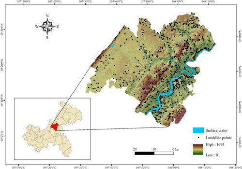
Zhong County is located in the eastern part of Chongqing and the centre of the Three Gorges Reservoir area, between 107°3′∼108°14′ east longitude and 30°03′∼30°35′ north latitude. Zhong County has the terrain of ‘three mountains and two troughs’, which is a deep hill and shallow hill with mountains, with an altitude of 8–1684 m. The terrain is composed of three anticlines of Jinhua Mountain, Fangdou Mountain, and Maoer Mountain, and two synclines of Bashan and Zhongzhou, which is a typical hilly landform. The lithology of the landslide stratum comprises Quaternary landslide accumulation soil, mainly consisting of silty clay with small amounts of sand and mudstone fragments. The underlying bedrock is predominantly composed of sandstone and mudstone from the Upper Jurassic Penglaizhen Formation. The reservoir area experiences a subtropical humid monsoon climate, with an average annual rainfall ranging from 1100 to 1400 mm, mostly concentrated in the summer season. Due to its location in the centre of rainstorm, the area can experience maximum daily rainfall of up to 230.8 mm, and the maximum three-day rainfall of 355.3 mm, often in the form of rainstorm and prolonged rainfall. Groundwater in the reservoir area is abundant and tends to fluctuate in sync with rainfall and reservoir water level. During times of reservoir elevation, the water can pour into the landslide. Figure 1 shows the geographical location and distribution of historical landslide points in the study area.

Figure 1. Geographical location and historical landslide events distribution of Zhong County.

2.2. Data source

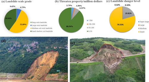
The historical landslide data used in the study consisted of 942 records from the period between 2000 and 2016. These data were obtained by converting the landslide disaster data table provided by the Chongqing Geological Environment Monitoring Station into point data. The majority of the landslides were categorized as small shallow soil and medium soil rock landslides (as illustrated in Figure 2(a)), and nearly 80% of the landslide hazard level is low (as illustrated in Figure 2(c)), posing threats to human properties ranging from several hundred thousand to tens of millions in value, and causing significant impacts on production and livelihoods of local communities (as shown in Figure 2(b)). Figures d and e present the field maps of two of these landslides. Elevation data was obtained from Aster satellite spatial resolution of 30 m Digital elevation model (DEM) raster data. Landsat 8 OLI satellite image (2016) was downloaded from geospatial data cloud with a spatial resolution of 30 m. The lithology was derived by vectorizing the geological map obtained from the National Geological Data Centre at a scale of 1:200,000. The rainfall data were obtained using the ArcGIS spatial interpolation method from the rainfall data table of the Chongqing Meteorological Bureau. The road data was derived from Chongqing Transportation Commission, the river network data was derived from Chongqing Water Resources Bureau, and the land use data and administrative division data were obtained from the Geographic National conditions monitoring cloud platform. The accuracy of the four types of data was 1:100,000. POI kernel density data from Baidu API crawler, and the data type was table data.

Figure 2. Historical landslide data introduction ((d) Wachangwan Landslide; (e) Bantai Landslide).

3. Spatial database of landslide conditioning factors

3.1. Conditioning factors

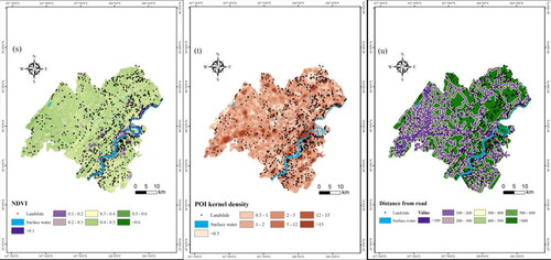
The formation of landslides is a complex process, and the factors that contribute to landslides vary from region to region (Reichenbach et al. 2018). On the basis of summarizing predecessors’ experience (Kalantar et al. 2018; Wang, Sun, et al. 2020; Wang, Feng, et al. 2020; Sun et al. 2022) and combining with the topography and landslide development conditions of Zhong County, we selected 21 conditioning factors, including four types of landslide evaluation indexes, to construct a landslide susceptibility evaluation index system. Specific conditioning factors are as follows: 1) Topographic and landform, including Elevation, Slope, Aspect, Slope position, Curvature, Topographic relief, Micro-landform, Plan curvature, Profile curvature, sediment transport index (STI), hydrodynamic index (SPI), roughness index (TRI), and topographic humidity index (TWI); 2) Geological conditions, including Lithology and Slope structure; 3) Environmental conditions, including Annual average rainfall, Distance from river, Land use and normalized difference vegetation index (NDVI); 4) Human activities, including POI kernel density, Distance from road. The influence direction of each factor on landslide occurrence is shown in Table 1.

Table 1. The influence direction table of conditioning factors on landslide.

Type	Conditioning factors	The influence direction of landslide occurrence
Topography and landform	Elevation	Affect the intensity of human activities, the distribution of rainfall.
	Slope/°	The steepness of the slope affects the pushing and moving of the debris.
	Aspect	Affect the sunshine hours of the slope, thus affecting the growth of vegetation.
	Slope position	There are differences in groundwater distribution, rock dip angle, and lithology of slopes with different slope positions.
	Curvature	Affect the velocity of soil erosion and surface runoff on the slope.
	Topographic relief/m	Macroscopic index of regional terrain characteristics.
	Micro-landform	The smallest geomorphological unit affects slope stability.
	Plan curvature	The slope perpendicular to the direction of the maximum slope affects surface runoff and soil erosion.
	Profile curvature	Reflect the bending change of the surface in the vertical direction, which affects the soil deposition and water flow velocity.
	STI	It is a quantitative expression of the sediment transport capacity of surface water to sediment. The larger the value, the stronger the sediment transport capacity.
	SPI	Reflect the velocity of running water, the greater the value, the stronger the erosion ability of running water.
	TRI	It is the ratio of the earth’s surface area to the projected area of the region, which describes the surface morphology macroscopically.
	TWI	Physical indicators reflecting the influence of topography on runoff direction and accumulation
Geological conditions	Lithology	The hardness of lithology is an important factor affecting the occurrence of landslides.
	Slope structure	It is the relationship type between slope direction and rock strata tendency, and is an important factor affecting slope stability.
Environmental conditions	Annual average rain/mm	Direct erosion of slope, scour the surface.
	Distance from river/m	The erosion of the river affects the stability of the slope. The closer to the river, the higher the water content of the slope and the more serious the softening.
	Land use	Reflect the degree of human transformation of the surface.
	NDVI	Reflect the vegetation coverage and affect the stability of the slope.
Human activities	POI kernel density	Reflect the intensity of human activities.
	Distance from road/m	Affect the stability and continuity of slope toe.

3.2. Data preprocessing

Thirteen factors, such as Elevation, Slope, Aspect, Slope position, Curvature, Topographic relief, Micro-landform, Plan curvature, Profile curvature, STI, SPI, TRI, and TWI, were derived from DEM data using ArcGIS. The Lithology and Slope structure data were obtained by vectorization of 1:200,000 geological map. The distance to the river and the distance to the road were obtained by multi-loop buffering. NDVI was obtained from Landsat 8 OLI satellite images calculated by ArcGIS. The conditioning factors were reclassified using the natural breakpoint method and expert experience. Refer to Table 2 for the specific classification standards.

Table 2. Landslide conditioning factor classification.

Attribution category	Conditioning factors	Number of stages	Classification standard
Topography and landform	Elevation/m	9	1. >8 ∼ 214; 2. >214 ∼ 311; 3. >311 ∼ 402; 4. >402 ∼ 480; 5. >480 ∼ 557; 6. >557 ∼ 661; 7. >661 ∼ 805; 8. >805 ∼ 1088; 9. >1088 ∼ 1674
	Slope/°	5	<7.8; 2. >7.8 ∼ 15; 3. >15 ∼ 22.3; 4. >22.3 ∼ 31.5; 5. >31.5 ∼ 66
	Aspect	9	1. Plane; 2. North; 3. Northeast; 4. East; 5. Southeast; 6. North; 7. Southwest; 8. West; 9. Northwest
	Slope position	6	1. Valley floor; 2. Down slope; 3. Flat slope; 4. Middle slope; 5. Hillside; 6. Ridge of mountains
	Curvature	5	1. <-2; 2. >-2∼-0.5; 3. >-0.5 ∼ 0.5; 4. >0.5 ∼ 2; 5. >2
	Topographic relief/m	6	1. >0 ∼ 20; 2. >20 ∼ 30; 3. >30 ∼ 40; 4. >40 ∼ 50; 5. >50 ∼ 80; 6. >80 ∼ 158
	Micro-landform	10	1. Canyon/ deep stream; 2. Water system/shallow valley on the middle slope; 3. Upland water systems/sources; 4. ‘U’ shaped valley; 5. Plain; 6. Open slope; 7. Upper slope/valley floor; 8. Local ridge in the valley; 9. A ridge/hill in the middle slope of the plain; 10. High up on a hill/ridge
	Plan curvature	5	1. <-1; 2. >-1∼-0.5; 3. >-0.5 ∼ 0.5; 4. >0.5 ∼ 2; 5. >2
	Profile curvature	5	1. <-1; 2. >-1∼-0.5; 3. >-0.5 ∼ 0.5; 4. >0.5 ∼ 2; 5. >2
	STI	6	1. <20; 2. >20 ∼ 40; 3. >40 ∼ 70; 4. >70 ∼ 100; 5. >100 ∼ 200; 6. >200
	SPI	5	1. <7; 2. >7 ∼ 14; 3. >14 ∼ 22; 4. >22 ∼ 40; 5. >40
	TRI	5	1. <1; 2. >1 ∼ 1.1; 3. >1.2 ∼ 1.3; 4. >1.3 ∼ 1.4; 5. >1.5
	TWI	6	1. <5; 2. >5 ∼ 7; 3. >7 ∼ 9; 4. >9 ∼ 12; 5. >12 ∼ 17; 6. >17
Geological conditions	Lithology	8	1. T3xj; 2. T21; 3. T2b; 4. T1d-j; 5. J3sn; 6. J3p; 7. J2s; 8. T1z-2x
	Slope structure	6	1. Forward slope; 2. Oblique dip slope; 3. Oblique slope; 4. Cross slope; 5. Reverse slope; 6. Flat stack slope
Environmental conditions	Annual average rain/mm	7	1. <1250; 2. >1250 ∼ 1280; 3. >1280 ∼ 1300; 4. >1300 ∼ 1330; 5. >1330 ∼ 1350; 6. >1350 ∼ 1380; 7. >1380
	Distance from river/m	11	1. <100; 2. >100 ∼ 200; 3. >200 ∼ 300; 4. >300 ∼ 400; 5. >400 ∼ 500; 6. >500 ∼ 600; 7. >600 ∼ 700; 8. >700 ∼ 800; 9. >800 ∼ 900; 10. >900 ∼ 1000; 11. >1000
	Land use	8	1. Land transportation; 2. Residental land; 3. Garden land; 4. Industrial and mining storage land; 5. Forest land; 6. Water and water conservancy facilities; 7. Cultivated land; 8. Grass field
	NDVI	7	1. <0.1; 2. >0.1 ∼ 0.2; 3. >0.2 ∼ 0.3; 4. >0.3 ∼ 0.4; 5. >0.4 ∼ 0.5; 6. >0.5 ∼ 0.6; 7.>0.6
Human activities	POI kernel density	7	1. <0.5; 2. >0.5 ∼ 1; 3. >1 ∼ 2; 4. >2 ∼ 5; 5. >5 ∼ 12; 6. >12 ∼ 15; 7. >15
	Distance from road/m	7	1. <100; 2. >100 ∼ 200; 3. >200 ∼ 300; 4. >300 ∼ 400; 5. >400 ∼ 500; 6. >500 ∼ 600; 7.>600

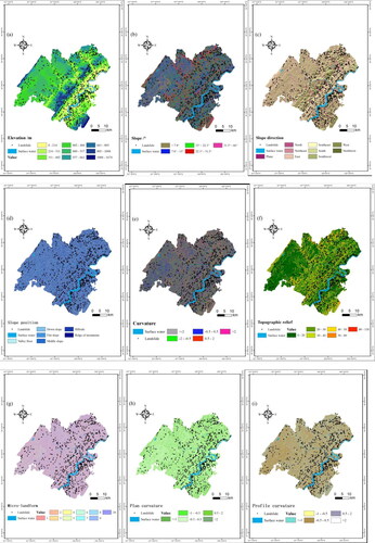
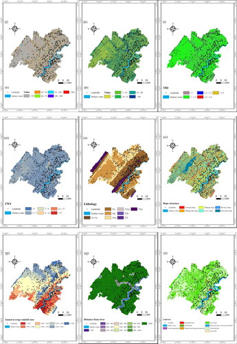
With 30 m*30m grid unit as the basic unit of landslide susceptibility evaluation, a geo-spatial database of landslide conditioning factors was established and visualized in Figure 3.

Figure 3. Thematic layer of landslide conditioning factors.

4. Research methods

4.1. Research idea

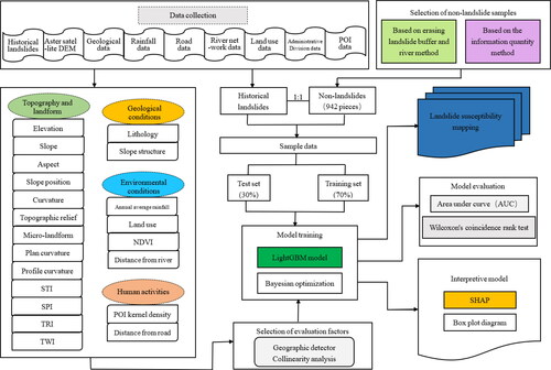
The process of establishing landslide susceptibility zoning in this paper is illustrated in Figure 4. First, a spatial database of landslide conditioning factors is collected and established. A total of 21 conditioning factors are selected from four aspects of topography and landform, geological conditions, environmental conditions, and human activities, and the accuracy of all data is maintained at 30 m * 30 m by resampling. Considering that landslide susceptibility is a binary classification problem, the selection of positive and negative landslide samples in a 1:1 ratio ensures sample balance. Additionally, the 1:1 extraction method is commonly used in similar studies (D. Sun et al. 2021; Hong et al. 2017; Huang et al. 2020). Therefore, based on the traditional method (the method of erasing landslide buffer and river) and the information quantity method, 942 negative samples are extracted, respectively, in 1:1 ratio, and the factors with weak interpretation of landslide are eliminated by using the geographical detector. Then the LightGBM model is optimized by Bayesian optimization to get the landslide susceptibility model of Zhong County. Finally, SHAP method is used to explain the decision-making process of the model.

Figure 4. Flow chart of the methodology.

4.2. Landslide susceptibility zoning

4.2.1. Information quantity method

Both the information method and the frequency ratio method belong to the probability statistical model, but there are differences between them. The frequency ratio method (Li et al. 2017) is a statistical method to calculate the frequency ratio between geological disasters and evaluation factors, indicating the degree of correlation between the two. The more the distribution of disaster points, the greater the probability of occurrence. However, there is a lack of in-depth study on the mechanism of event occurrence. This method is only applicable to areas with a large number of samples and a long time series of events. The information quantity method is a statistical evaluation method derived from the quantitative description of information in information theory (Klüver 2011). In general, a higher probability of landslide occurrence is associated with a lower amount of event information, whereas a lower probability of occurrence is associated with a higher amount of event information. Additionally, different geographical environments can also contribute to the occurrence of geological disasters. The information method comprehensively calculates the probability of landslide occurrence by quantifying the information required to reduce the uncertainty of the event, as well as considering the information value contributed by various evaluation factors in relation to the occurrence of geological disasters (Clerici et al. 2002). The information method combines various influencing factors that affect landslide occurrence, resulting in more reliable results. The process of calculating the factor information value by information method is as follows:

1. Calculate the amount of information provided by each factor $x_i$ for each level of landslide event $(H),$ that is:

(1) $$I\left(x_i,H\right)=ln\frac{N_i/N}{{\mathrm{S}}_i/S}$$(1)

where $N_i$ is the number of units of geological disaster occurring in the evaluation factor $X_i;$$N$ is the total number of units containing geological hazard distribution in the study area; $S_i$ is the number of units containing the evaluation factor $X_i$ in the study area. $S$ is the total number of evaluation units in the study area.

• Calculate the total information quantity value in each evaluation unit. Using the results of the total amount of information in ArcGIS median to make Zhong County landslide susceptibility model. The greater the information quantity value, the greater the possibility of landslide. If the information quantity value is zero, it means that the possibility of landslide in this area is zero.

4.2.2. Geographical detector

In order to improve the effectiveness of the model, the geographical detector is used to analyse the landslide conditioning factors and eliminate the conditioning factors that explain the probability of landslide occurrence in Zhong County to a low degree. Geographical detector is a tool to detect the spatial differentiation of independent variables and dependent variables. Compared with other analysis methods, geographical detector can quickly detect independent variables that have an important impact on dependent variables, including differentiation and factor detection, interaction detection, risk area detection, and ecological detection (D. Sun et al. 2021). This article mainly uses its factor detection part.

In factor detection, Y is the dependent variable and X is the independent variable, which is used to detect to what extent a factor X explains the spatial differentiation of Y. The formula is: (2) $$q=1-\frac{\sum _{h=1}^L{N}_h{Q}_{\mathrm{h}}^2}{N_Q^2}=1-\frac{\mathit{SSW}}{\mathit{SST}}$$(2) where h = 1, 2, …, L is the stratification of variable Y or factor X; $N_h$ and N are the sample and variance of the h layer, respectively. SSW and SST are the sum of in-layer variances and the sum of total sample variances, respectively. The range of Q is [0, 1], and the larger the value of q is, the stronger the interpretation of factor X on dependent variable Y is. When q = 0, it indicates that factor X does not affect dependent variable Y at all.

4.2.3. LightGBM principle and Bayesian parameter optimization

LightGBM (X. Sun et al. 2020) is an efficient GBDT algorithm proposed by Microsoft team. LightGBM algorithm adopts two strategies to obtain great advantages.

1. Leaf growth strategy with depth limitation is used (see Figure 5). By looking for the leaf with the largest gain of splitting information among all the current leaves, the classification accuracy of the algorithm is improved by further splitting and cycling.

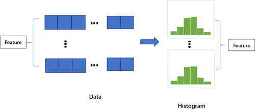
2. Histogram algorithm is used to find the optimal segmentation point (see Figure 6). First, the continuous floating-point data is discretized into n integers, and a histogram of width n is established at the same time. Then, the discrete value is used as the index to accumulate statistics.

Figure 5. Leaf-by-leaf growth strategy.

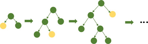
Figure 6. Histogram algorithm.

Bayes optimization algorithm is a very effective global optimization algorithm based on Bayes theorem, with probabilistic surrogate model and acquisition function as the core part (Taheri and Mammadov 2013), which can quickly and accurately find the optimal solution of complex objective function with less objective function evaluation.

The expression of Bayes’ theorem is: (3) $$P\left(f\right|D_{1:t})=\frac{P\left(D_{1:t}\right|f\left)P\right(f)}{P\left(D_{1:t}\right)}$$(3) where $f$ is the objective function, $D_{1:t}$ is observed association, $P\left(D_{1:t}\right|f)$ is the likelihood distribution of y, $P(f)$ is the prior probability distribution of $f,$ and $P\left(f\right|D_{1:t})$ is the posterior probability distribution of $f.$

4.3. SHAP interpretation model

Although LightGBM algorithm can obtain a prediction model with higher accuracy, LightGBM is almost a black box model, and its interpretation method is poor in the model. In order to better analyse the decision-making process of the model, SHAP interpretation model is introduced to explain the internal process of Landslide susceptibility model. SHAP (Sagi and Rokach 2021)is a kind of additive explanative model built by Lundberg inspired by cooperative game theory in 2017. By calculating the SHAP value of each feature variable, the influence of each feature and its positive or negative effect can be reflected, thereby explaining the prediction process of the model. This allows for a better understanding of how each feature contributes to the model’s predictions.

SHAP algorithm is widely used in complex machine learning model because of its powerful data visualization function. In this article, the decision process of LightGBM model is analysed by combining the three visual graphs of SHAP interpretability: (1) The scatter plot of characteristic density, which reflects the importance ranking of conditioning factors and the overall positive and negative relationship between conditioning factors and landslide. (2) Partial dependence graph, which analyses the influence direction of single factor on landslide in detail from the local perspective. (3) Waterfall diagram, which shows the contribution direction of the factors to the landslide from a global perspective.

5. Comparative analysis of landslide susceptibility evaluation

5.1. Conditioning factors information quantity

The information quantity value of each factor is obtained according to the calculation equation of landslide quantity, grid area, and information quantity corresponding to each level of each factor, as shown in Table 3. The total information quantity value is calculated using ArcGIS, and the natural breakpoint method and expert experience method are used for classification to obtain the susceptibility partition of the information quantity model, as shown in Figure 7.

Figure 7. The landslide susceptibility zoning map based on the information method.

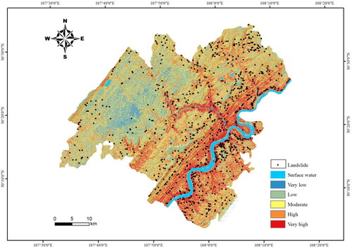
Table 3. Evaluation factor information table.

Factors	Classification	Landslide events/one	Information quantity value	Factors	Classification	Landslide events/one	Information quantity value
Elevation	1	125	0.521	TRI	1	118	0.097
	2	211	0.532		2	793	−0.009
	3	174	0.318		3	20	−0.223
	4	166	−0.249		4	9	0.158
	5	107	−0.738		5	2	0.037
	6	102	−0.039	TWI	1	356	0.023
	7	50	0.102		2	348	−0.109
	8	7	−1.290		3	144	0.185
	9	0			4	70	0.138
Slope	1	131	−0.587		5	22	0.049
	2	337	0.090		6	2	−0.719
	3	274	0.246	Lithology	1	55	−0.084
	4	156	0.167		2	6	−0.185
	5	44	−0.169		3	0
Aspect	1	3	−0.883		4	0
	2	126	0.169		5	222	−0.038
	3	101	−0.099		6	299	−0.076
	4	112	−0.074		7	223	−0.018
	5	110	−0.075		8	137	0.420
	6	125	0.102	Slope structure	1	102	0.068
	7	120	0.070		2	236	0.082
	8	135	0.032		3	153	0.116
	9	110	−0.104		4	317	0.069
Slope position	1	371	0.121		5	71	0.213
	2	73	−0.006		6	63	−0.795
	3	7	−1.349	Annual average rainfall	1	112	0.474
	4	130	0.103		2	206	0.292
	5	53	−0.110		3	165	0.151
	6	308	−0.089		4	184	−0.319
Curvature	1	61	0.042		5	127	−0.092
	2	278	0.129		6	122	−0.178
	3	337	−0.012		7	26	−0.390
	4	223	−0.090	Distance from river	1	12	−0.877
	5	43	−0.229		2	15	0.433
Topographic relief	1	429	−0.164		3	16	0.576
	2	287	0.248		4	29	1.189
	3	139	0.155		5	23	0.955
	4	60	0.102		6	17	0.664
	5	25	−0.385		7	22	0.924
	6	2	−0.232		8	18	0.720
Micro-landform	1	393	0.145		9	16	0.607
	2	23	0.026		10	14	0.475
	3	40	0.078		11	760	−0.092
	4	68	0.051		1	13	0.919
	5	0			2	4	0.592
	6	24	0.284		3	62	0.687
	7	56	−0.131		4	2	−0.232
	8	57	0.450		5	453	−0.018
	9	22	−0.010		6	20	−0.580
	10	259	−0.248		7	387	−0.035
Plan curvature	1	65	0.196		8	1	−0.877
	2	119	0.031	NDVI	1	7	−1.557
	3	586	−0.015		2	20	0.240
	4	167	−0.025		3	42	0.298
	5	5	−0.335		4	159	−0.102
Profile curvature	1	65	−0.282		5	571	0.020
	2	115	−0.062		6	143	0.126
	3	521	0.011		7	0
	4	225	0.113	POI kernel density	1	41	−0.229
	5	16	−0.086		2	121	−0.015
STI	1	719	−0.077		3	344	−0.067
	2	113	0.239		4	297	0.029
	3	56	0.462		5	66	0.075
	4	18	0.367		6	11	0.185
	5	24	0.563		7	62	0.418
	6	12	−0.214	Distance from road	1	199	0.166
SPI	1	222	−0.395		2	130	−0.028
	2	203	0.062		3	97	−0.123
	3	98	0.119		4	80	−0.127
	4	105	0.144		5	77	0.020
	5	314	0.255		6	60	−0.040
	–	–	–		7	299	−0.007

5.2. Selection of training and test samples

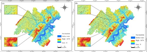
There are 942 historical landslide events in the study area. Based on the previous experience (Liao et al. 2022), this article extracts the non-landslide units by two methods based on the grid evaluation unit. The first method is the method of erasing landslide buffer and river, which is referred to as the traditional method (as shown in Figure 8(A)). The distribution of negative samples is shown in Figure 9(A). The second method, the information quantity method, involved using the total information value calculated by the information quantity method to create a landslide susceptibility zoning diagram. From the very low and low susceptibility areas, 942 non-landslide samples were selected. The specific processing process is shown in Figure 8(B), and the distribution of non-landslide events is shown in Figure 9(B).

Figure 8. Flow chart of training and test sample selection (A is the traditional method to select non-landslides; B is the information quantity method to select non-landslides).

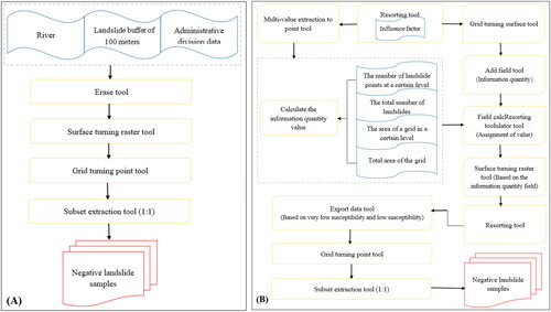
Figure 9. Negative sample distribution (A is the traditional method to select non-landslides; B is the information quantity method to select non-landslides).

5.3. Conditioning factors screening and collinearity analysis

The factor detector is an essential tool for assessing and exploring spatial stratification heterogeneity and spatial pattern attributes. It mainly measures the degree of interpretation of independent variables to dependent variables by the size of q value. Luo and Liu (2018) was the first to apply geographical detector to landslide susceptibility evaluation model, which objectively analysed the relative importance of landslide factors and provided a reference for the allocation of weights. Subsequently, many scholars used q value to quantitatively detect the spatial correlation between landslide and landslide factors (Jia et al. 2021; Q. Lin and Wang 2018; Zhou et al. 2021), further confirming the significant role of geographical detector in factor detection. Building upon this, this study utilizes the p value to explore the spatial distribution similarity intensity between the independent and dependent variables, and identifies important landslide influencing factors through screening. When the dependent variable was composed of negative samples through traditional selection, Land use, NDVI, Curvature, Profile curvature, TWI, Aspect, Distance from road, Plan curvature, and TRI were eliminated, and 12 conditioning factors were retained. When the negative samples were chosen using the information content method to form the dependent variable, the Distance from road factor was excluded, and 20 evaluation conditioning factors were retained. The outcomes are presented in Table 4.

Table 4. Analysis table of collinearity.

Conditioning factors	Collinearity analysis based on the traditional method		Collinearity analysis based on the information quantity method
	$\mathit{TOL}$	${\mathit{VIF}}_j$	$\mathit{TOL}$	${\mathit{VIF}}_j$
Lithology	0.940	1.064	0.912	1.097
Micro-landform	0.355	2.814	0.333	3.001
SPI	0.480	2.085	0.261	3.827
STI	0.707	1.414	0.512	1.954
Slope structure	0.918	1.089	0.733	1.365
Slope position	0.392	2.552	0.206	4.859
Slope	0.422	2.371	0.225	4.437
Distance from river	0.837	1.195	0.649	1.541
Annual average rainfall/mm	0.464	2.153	0.434	2.303
Elevation	0.413	2.419	0.372	2.690
Topographic relief	0.471	2.123	0.453	2.207
POI kernel density	0.948	1.055	0.932	1.073
Aspect			0.918	1.089
Plan curvature			0.434	2.305
Profile curvature			0.372	2.687
TWI			0.218	4.593
TRI			0.978	1.023
NDVI			0.784	1.275
Land use			0.705	1.418
Curvature			0.151	6.636

To address the issue of multicollinearity, which can affect the reliability of the model results when there is a high correlation between independent variables, this study conducts a collinearity analysis using SPSS software. The severity of multicollinearity is measured using the variance inflation factor (${\mathit{VIF}}_j$) and tolerance (TOL) values. If

${\mathit{VIF}}_j$ ≥ 10 or TOL < 0.1, it indicates the presence of multicollinearity between the independent variables (Kock and Lynn 2012; L. Ma et al. 2016). The factors screened by geographical detector are used in the collinearity analysis, and the results, as shown in Table 5, indicate that there is no collinearity problem among the 21 influencing factors. This suggests that the factor selection approach used in this study is feasible.

Table 5. Results of the geographic detector.

Determine the dependent variable based on the traditional method			Determine the dependent variable based on the information quantity method
	q Statistic	p Value		q Statistic	p Value
Elevation	0.3112	0.000	Elevation	0.0933	0.0000
Slope	0.2635	0.000	Slope	0.0337	0.0000
SPI	0.2600	0.000	Distance from river	0.0323	0.0000
Slope structure	0.1670	0.000	Slope structure	0.0310	0.0000
Topographic relief	0.1621	0.000	Annual average rainfall	0.0249	0.0000
Slope position	0.1419	0.000	SPI	0.0238	0.0000
Micro-landform	0.1335	0.000	Micro-landform	0.0192	0.0000
Annual average rainfall	0.1303	0.000	Lithology	0.0173	0.0000
STI	0.1013	0.000	Slope position	0.0149	0.0000
Curvature	0.1004	0.000	STI	0.0121	0.0179
Profile curvature	0.0758	0.000	POI kernel density	0.0120	0.0156
Distance from river	0.0734	0.000	Topographic relief	0.0117	0.0029
Plan curvature	0.0607	0.000	Land use	0.0095	0.1115
Lithology	0.0540	0.000	NDVI	0.0092	0.0316
Land use	0.0506	0.000	Curvature	0.0083	0.0063
TWI	0.0477	0.000	Profile curvature	0.0068	0.0345
TRI	0.0252	0.000	TWI	0.0044	0.3229
POI kernel density	0.0194	0.000	Aspect	0.0036	0.6232
NDVI	0.0187	0.000	Distance from road	0.0031	0.4975
Aspect	0.0166	0.000	Plan curvature	0.0029	0.4242
Distance from road	0.0085	0.0204	TRI	0.0026	0.4951

5.4. Landslide susceptibility evaluation results

The data sets obtained from two methods of selecting non-landslide samples are applied to LightGBM model to predict the spatial distribution of landslide occurrence probability in Zhong County. The susceptibility mapping based on the traditional non-landslides LightGBM model is categorized into five levels: very low (0.12–0.37), low (0.37–0.52), moderate (0.52–0.66), high (0.66–0.76), and very high (0.76–0.9). The susceptibility mapping based on the information non-landslides LightGBM model are categorized into five levels: very low (0.003–0.33), low (0.33–0.57), medium (0.57–0.76), high (0.76–0.95), and very high (0.95–1) susceptibility zones. See Figure 10 for details.

Figure 10. Landslide susceptibility mapping (A is based on the traditional non-landslides LightGBM model; B is based on the information non-landslides LightGBM model).

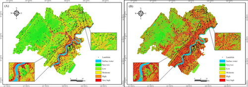
In the LSM based on the traditional method, the majority of Zhong County falls within the very low and low susceptibility categories, with a concentration in the northern and central regions. Areas with high landslide susceptibility are predominantly located near rivers. The number of landslides in the very high-high susceptibility zone accounts for 16.89% of the total number of historical landslides in the study area, with a landslide density of 2.25. Conversely, the number of landslides in the very low-low susceptibility area accounts for 61.97% of the total number of historical landslides, with a landslide density of 0.5. Notably, most landslides occurred in extremely low-low-prone areas. Although the density of landslides in extremely high-prone areas is high, the actual number of landslides is comparatively low, suggesting a discrepancy between the susceptibility assessment and the observed data.

In contrast, the LSM based on the information quantity method indicates that most areas in Zhong County are classified as very high and high susceptibility zones, particularly in the vicinity of dug hills, valleys, and rivers. The number of landslides in the very high-high susceptibility zone accounted for 77.92% of the total number of historical landslides, with a landslide density of 1.23. The very low-low susceptibility area is located in the west of Zhong County, with the number of landslides accounting for 13.59% of the total historical landslides and a landslide density of 0.34. Additionally, the landslide density increases by more than five times from 0.14 to 0.78, as shown in Table 6.

Table 6. Landslide susceptibility mapping statistical table.

Susceptibility grade	The traditional non-landslides LightGBM model			The information non-landslides LightGBM model
	Number of landslides/one	Area ratio/%	Landslide density/ (a. km²)	Number of landslides/ one	Area ratio/%	Landslide density/ (a. km²)
Very low	113	33.02	0.15	80	25.90	0.14
Low	226	28.95	0.35	48	10.66	0.20
Moderate	259	21.14	0.56	80	10.61	0.34
High	219	13.07	0.76	234	23.64	0.45
Very high	125	3.82	1.49	500	29.17	0.78

Interestingly, the landslide density in the very high-high susceptibility zone based on the information non-landslides LightGBM model is low, which contradicts the results obtained from the susceptibility mapping based on the traditional method of selecting negative samples. Moreover, the majority of landslides are found in the very high-high susceptibility zone, accounting for more than 75% of the total number of historical landslides, which is more consistent with the actual situation of the wide distribution range of local landslides. After conducting a comprehensive comparison, it can be concluded that the landslide susceptibility zoning map based on the information non-landslides LightGBM model yields better and more consistent prediction results.

5.5. Model evaluation

On the basis of previous studies (Myronidis et al. 2016; Taalab et al. 2018), the training and test samples were selected in a ratio of 7:3. The model iterations were set to 100, and the random_state was set to 52. The optimization parameters of the two models are presented in Table 7. Max_depth is used to control the maximum depth of the tree in order to prevent overfitting. Min_child_samples help specify the minimum sum of sample weights in a node. N_estimators refer to the number of base learners, where a larger value indicates a more complex model. Num_leaves represent the number of leaf nodes, which directly impacts the model’s complexity.

Table 7. Bayesian parameter optimization table.

Model	Max_depth	Min_child_samples	N_estimators	Num_leaves
Parameter threshold	(2, 10)	(2, 100)	(10, 1000)	(5, 1000)
The traditional non-landslides LightGBM model	5	24	70	442
The information non-landslides LightGBM model	3	29	865	966

To measure the accuracy of the models, accuracy rate, recall rate, F1-score, test set AUC, and training set AUC are used as indicators, where higher values indicate higher accuracy. As shown in Table 8, all measurement indices of the information non-landslides LightGBM model are better than the other model, with a significant difference in values between the two models. Therefore, the information non-landslides LightGBM model is more accurate for predicting landslide susceptibility.

Table 8. Accuracy evaluation table of LightGBM model.

Model	Accuracy rate	Recall rate	Accuracy rate	F1-score	Test set AUC	Training set AUC
The traditional non-landslides LightGBM model	62.95%	62.95%	63.60%	62.95%	0.705	0.783
The information non-landslides LightGBM model	96.24%	88.89%	92.58%	92.42%	0.964	0.960

To further verify the differences between the two models, Wilcoxon’s coincidence rank test is used in this study to analyse whether there are statistically significant differences in the results of the models. First, the results of the model prediction do not conform to the normal distribution by SPSS, so the paired samples of non-parametric test are used. We assume that there is no significant difference between the median and zero of the difference between the predicted results of the two models. Through the inspection finds that accepting the hypothesis of the p value is 0, that assumption is not in conformity with the two models exist significant difference. Therefore, statistically, the influence of two kinds of sample data of the model is also significant differences.

6. Discussion

6.1. Importance analysis of conditioning factors

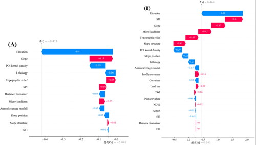
The SHAP Summary Plot is a way to visualize the importance of different features in a model and how they contribute to the output of the model. In the figure, the abscissa is SHAP value. If SHAP value > 0, it indicates that the variable has an increasing effect on the occurrence of landslide. if SHAP value < 0, it indicates that the variable has a decreasing effect on the occurrence of landslide. Each row represents a characteristic variable, and each dot represents a sample. The redder the dot colour is, the larger the variable value is. The bluer the dot colour is, the smaller the characteristic value is.

Based on the traditional non-landslides LightGBM model, the top six ranking of conditioning factors are: Elevation > Slope > SPI > Distance from river > Lithology > Annual average rainfall. Based on the information non-landslides LightGBM model, the top six influential factors are as follows: Elevation > SPI > Slope > Slope structure > Micro-landform > Topographic relief. Both models regard Elevation as the most important factor causing the occurrence of landslide in Zhong County. In addition, Slope and SPI are also the main factors leading to the occurrence of landslides in Zhong County (Factor importance ranking Figure 11).

Figure 11. SHAP feature summary (A is the traditional non-landslides LightGBM model; B is the information non-landslides LightGBM model).

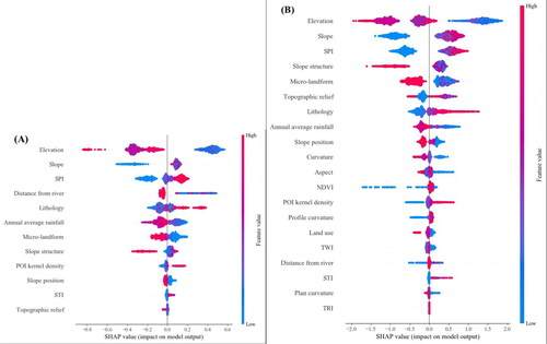
There are some similarities and differences in the importance ranking of decision factors in the two models. For the top three factors, the decision results of the two models are roughly the same, indicating that Elevation, Slope and SPI are important factors for the occurrence of landslide in Zhong County. However, the rankings of other factors differ significantly due to the varying number of conditioning factors analysed by the two models. As a result, it is challenging to conduct a comprehensive analysis of the differences in factor importance ranking.

6.2. Partial factor explanation

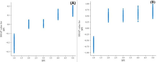
Zhong County is characterized by hilly terrain with large slopes, making it highly susceptible to landslides. The elevation in the area ranges from 8 to 1674 m, as shown in Figure 12. The figure indicates that landslides mainly occur at elevations between 8 and 402 m above sea level. At lower elevations, human activities such as excavation and cutting have resulted in soil damage, reducing slope stability and increasing the likelihood of landslides. However, at higher elevations, where human activity is less frequent and vegetation coverage is higher, the risk of landslides is lower. Figure 13 demonstrates that when the slope is less than 7.8°, the SHAP value is less than 0, while when the slope is greater than 7.8°, the SHAP value is >0. This is because the terrain is flatter in gentle slope areas, providing greater resistance to slope movement. In contrast, steep slope areas are more susceptible to slope movement, especially when combined with soil damage caused by human activity. This finding is consistent with previous studies. The SPI is a quantitative measure of surface water erosion, with larger values indicating stronger erosion ability of flowing water on the surface and shallow soil. Conversely, smaller values indicate weaker erosion ability of flowing water on the surface and shallow soil. As shown in Figure 14, when the SPI is less than 7, the erosion ability of flowing water on the surface is weak, resulting in a lower likelihood of landslides. In contrast, when the SPI is greater than 7, soil and water loss are more severe, the slope becomes less stable, and the likelihood of landslides increases. This finding is consistent with real-world observations.

Figure 12. Elevation local interpretation (A is the traditional non-landslides LightGBM model; B is the information non-landslides LightGBM model).

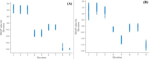
Figure 13. Slope local interpretation (A is the traditional non-landslides LightGBM model; B is the information non-landslides LightGBM model).

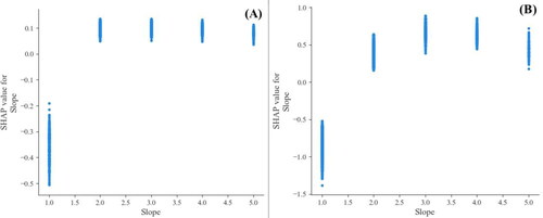
Figure 14. SPI local interpretation (A is the traditional non-landslides LightGBM model; B is the information non-landslides LightGBM model).

6.3. Local landslide interpretation

The SHAP feature waterfall plot can specifically show the contribution direction of the impact factor to the occurrence of local landslides. This article selects the Zhongjiayuan landslide occurred in Liangquan Village, Zhong County in 2012. The landslide caused 2 deaths and 2 injuries, and the teaching work of nearby schools was forced to stop, which had a great impact on local residents. The analysis of the influencing factors of the two models on the landslide is shown in Figure 15, and some of the factors are explained as follows.

Figure 15. SHAP waterfall plots (A is the traditional non-landslides LightGBM model; B is the information non-landslides LightGBM model).

Both models identify elevation as a negative contribution and slope as a positive contribution. Zhongjiayuan landslide is located in a valley with a low elevation and large relief surrounding it. Therefore, the altitude impedes the occurrence of landslides, and the slope promotes the occurrence of landslides. In general, the two models identify the same direction of the influence factors on landslide, but there is a big difference in the size of the specific impact. This indicates that different sample data will also lead to differences in the decision-making mechanism within the model. Although in general agreement, but there are big differences in details.

6.4. Analysis of data distribution structure

To analyse the differences in data distribution structure of the LightGBM model obtained by the two methods, this article employs box plots and scatter plots to examine the landslide predicted value (score) distribution structure and the landslide distribution in some factors. The following observations were made:

1. Figure 16 shows that there are no outliers in the data obtained by the two methods. However, the LightGBM model based on the information non-landslides LightGBM method has larger maximum and smaller minimum values, indicating that its predicted values are more dispersed and lengthwise extended compared to the traditional non-landslides LightGBM model. In addition, the predicted value distribution of the traditional non-landslides LightGBM model is more concentrated, which is also evident from Figure 17.

2. The median line based on the traditional non-landslides LightGBM model is biased to the lower quartile with the mean value distributed above the median line. This indicates that the values are mainly concentrated in the low-value region. On the other hand, the median line of the model based on the information non-landslides LightGBM method is biased towards the upper quartile, with the mean distributed below the median line and a large gap between them, indicating that most of the values of this model are concentrated in the higher value area. Therefore, the high susceptibility area of landslide susceptibility zoning based on the information non-landslides LightGBM model occupies the majority of the study area.

3. ArcGIS was used to generate a landslide scatter diagram by connecting model prediction results with landslide events, as shown in Figure 17. The figure reveals that the landslide units based on the traditional non-landslides LightGBM model are evenly distributed in clumps up and down. Conversely, the landslide events of the model based on the information non-landslides LightGBM method have a wide distribution range, but the data is mainly concentrated at the top, with the landslide units at the bottom more sparsely distributed. These findings suggest that the information non-landslides LightGBM model has a more accurate resolution of landslide units and a higher recognition accuracy of landslide areas.

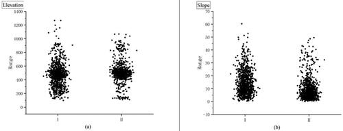
4. By connecting the two kinds of non-landslide sample data with some factors, the scatter plot of non-landslide samples based on elevation value and slope value is obtained, as shown in Figure 18. When observing the distribution pattern of non-landslide sample data selected based on the traditional method, a common feature is noticeable: a wider distribution range, a small part of concentrated, and most dispersed. While non-landslide sample data selected based on the information quantity method has a small distribution range, most concentrated, and a small part of dispersed. Taking the distribution characteristics of non-landslides in elevation as an example, the non-landslides selected based on the traditional method are centrally distributed in the range of 400–600 and 200–300 m, and some data are also distributed in other ranges. The majority of non-landslide samples selected through the information content method are centrally distributed in the range of 400–600 m, with some data scattered in a small range. Due to the significant problems of randomness and subjectivity in the traditional method, the selection rule of non-landslides is not obvious. Conversely, the information quantity method selects samples by calculating the information value of geological disasters, resulting in the distribution of non-landslide units having obvious rules in the conditioning factors.

Figure 16. Box plot of model prediction value.

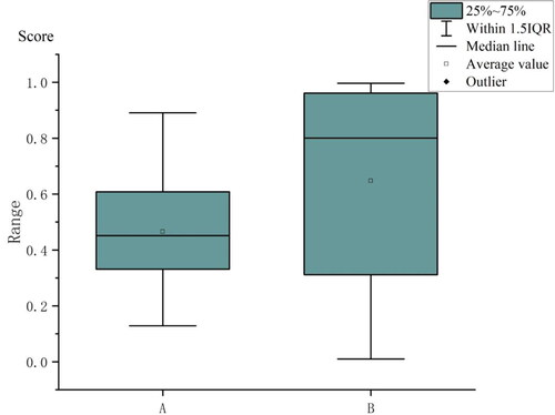
Figure 17. Landslide scatter plot based on predicted values. (Note: In the two maps, A is based on the traditional non-landslides LightGBM model; B is based on the information non-landslides LightGBM model, and Figure 17 uses ArcGIS to connect the model prediction results with the landslide points to generate a scatter plot).

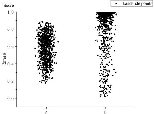
Figure 18. Non-landslide sample scatter plot based on elevation value and slope value. (Note: I in the two maps is the negative sample selected by the traditional method, and II is the negative sample selected by the information method. The two maps generate a scatter plot by connecting the elevation value and the slope value with the non-landslide sample, respectively).

6.5. Different selection methods of landslide sample analysis

Similar to previous research by other scholars (Liu et al. 2023), non-landslide samples in this study were selected using the information method. However, unlike previous studies, this study compared the impact of different samples on the same model, which allowed for a clear observation of changes in model accuracy. Furthermore, this study considered both collinearity among factors and the correlation between factors and landslides, in order to exclude any potential influence of factors on the model. Lastly, SHAP was used to provide explanations for the internal mechanism of the model’s decision-making process, enhancing our understanding of the model’s credibility and improving overall interpretability. Sample quality is the key to the data-driven landslide susceptibility model. Different sample data selection methods make non-landslide samples different in the distribution of evaluation factors, which in turn leads to differences in model accuracy and model decision-making. The information method for selecting non-landslide samples is advantageous compared to traditional methods, as it takes into account the landslide disaster situation, topography, and geology of the study area. This results in a more objective, scientific, and reasonable selection of sample data. As a result, the model accuracy and prediction results are improved. The information method holds great significance in obtaining high-quality sample data, which in turn enhances the reliability of the model and its subsequent analyses.

7. Conclusions

1. By comparing the two methods of selecting negative samples, it is found that the AUC of the test set based on the information method LightGBM model is increased by 25.9%, and more than 75% of historical landslides are located in extremely high-high prone areas. Therefore, selecting negative samples based on information quantity improves sample quality and model accuracy. As a result, the predicted results of the model are more consistent with the actual situation.

2. According to the interpretability of SHAP, Elevation, Slope and SPI are identified as the dominant factors of landslide occurrence in Zhong County by both models. Specifically, landslides were promoted when the altitude was between 8 and 400 meters, the slope was greater than 7.8°, and the SPI was greater than 7.

3. Different sample data not only lead to different in factor evaluation, model accuracy and prediction results, but also cause differences in the internal decision-making mechanism of the model. This highlights the importance of selecting high-quality sample data to build a reasonable model. The negative samples selected by the information quantity method can significantly improve the accuracy of the model and provide important reference value for future research.

Indeed, the selection of negative samples using the information method has been shown to significantly impact the accuracy of the model, leading to more consistent prediction results with the actual situation. This finding provides valuable insights for the reasonable selection of negative samples in future landslide susceptibility modelling in hilly areas.

However, it is acknowledged that there are limitations in this study. For instance, in reality, non-landslide samples may not always be exclusively located in very low-low-prone areas. The possibility of overfitting due to the selection of negative samples only from certain regions needs further investigation. Additionally, while the LightGBM model based on the information method predicts most of Zhong County as a high-prone area for landslides, field investigations could be conducted to confirm this conclusion and strengthen the credibility of the research findings.

In conclusion, this study serves as a preliminary exploration and further improvements and in-depth studies are warranted to overcome the limitations and enhance the reliability of the results. Combining theoretical insights with practical field investigations can contribute to a more comprehensive understanding of landslide susceptibility and improve the overall robustness of the research findings.

Authors’ contributions

Conceptualization, Haijia Wen and Deliang Sun; methodology, Deliang Sun and Xiaoqing Wu; software, Xiaoqing Wu; validation, Xiaoqing Wu and Qingyu Gu; formal analysis, Qingyu Gu; investigation, Xiaoqing Wu; resources, Deliang Sun; data curation, Deliang Sun and Xiaoqing Wu; writing—original draft preparation, Deliang Sun and Xiaoqing Wu; writing—review and editing, Haijia Wen; visualization, Xiaoqing Wu; supervision, Haijia Wen; project administration, Deliang Sun; funding acquisition, Deliang Sun. All authors have read and agreed to the published version of the manuscript.

Disclosure statement

No potential competing interest was reported by the authors.

Data availability statement

The datasets used or analysed during this study are available from the corresponding author on reasonable request.

Additional information

Funding

This work was supported by the Natural Science Foundation of Chongqing (CSTB2022NSCQ-MSX0594) and National Social Science Funds of China (Grant No. 22BJY140).

References

- Bentéjac C, Csörgő A, Martínez-Muñoz G. 2021. A comparative analysis of gradient boosting algorithms. Artif Intell Rev. 54(3):1937–1967.
- Brenning A. 2012. Spatial cross-validation and bootstrap for the assessment of prediction rules in remote sensing: the R package sperrorest. 2012 IEEE International Geoscience and Remote Sensing Symposium, p. 5372–75.
- Carrara A, Fausto G., editors. 1995. Geographical information systems in assessing natural hazards. Advances in natural and technological hazards research. Vol. 5. Dordrecht, Netherlands: Springer Netherlands.
- Chang Z, Huang J, Huang F, Bhuyan K, Meena SR, Catani F. 2023. Uncertainty analysis of non-landslide sample selection in landslide susceptibility prediction using slope unit-based machine learning models. Gondwana Res. 117:307–320.
- Chen W, Pourghasemi HR, Kornejady A, Zhang N. 2017. Landslide spatial modeling: introducing new ensembles of ANN, MaxEnt, and SVM machine learning techniques. Geoderma. 305:314–327.
- Clerici A, Perego S, Tellini C, Vescovi P. 2002. A procedure for landslide susceptibility Zonation by the conditional analysis method. Geomorphology. 48(4):349–364.
- ElShawi R, Sherif Y, Al-Mallah M, Sakr S. 2021. Interpretability in healthcare: a comparative study of local machine learning interpretability techniques. Comput Intell. 37(4):1633–1650.
- Hong H, Ilia I, Tsangaratos P, Chen W, Xu C. 2017. A hybrid fuzzy weight of evidence method in landslide susceptibility analysis on the Wuyuan Area, China. Geomorphology. 290:1–16.
- Hong H, Miao Y, Liu J, Zhu A-X. 2019. Exploring the effects of the design and quantity of absence data on the performance of random forest-based landslide susceptibility mapping. Catena. 176:45–64.
- Hong H, Pourghasemi HR, Pourtaghi ZS. 2016. Landslide susceptibility assessment in lianhua county (China): a comparison between a random forest data mining technique and bivariate and multivariate statistical models. Geomorphology. 259:105–118.
- Huan Y, Song L, Khan U, Zhang B. 2023. Stacking ensemble of machine learning methods for landslide susceptibility mapping in Zhangjiajie City, Hunan Province, China. Environ Earth Sci. 82(1):1–18.
- Huang F, Cao Z, Jiang S-H, Zhou C, Huang J, Guo Z. 2020. Landslide susceptibility prediction based on a semi-supervised multiple-layer perceptron model. Landslides. 17(12):2919–2930.
- Jia WJ, Wang MF, Zhou CH, Yang QH. 2021. Analysis of the spatial association of geographical detector-based landslides and environmental factors in the Southeastern Tibetan Plateau, China. PLoS One. 16(5):e0251776.
- Kalantar B, Pradhan B, Amir Naghibi S, Motevalli A, Mansor S. 2018. Assessment of the effects of training data selection on the landslide susceptibility mapping: a comparison between support vector machine (SVM), Logistic Regression (LR) and Artificial Neural Networks (ANN). Geomat Nat Hazard Risk. 9(1):49–69.
- Kavzoglu T, Teke A. 2022. Predictive performances of ensemble machine learning algorithms in landslide susceptibility mapping using random forest, extreme gradient boosting (XGBoost) and natural gradient boosting (NGBoost). Arab J Sci Eng. 47(6):7367–7385.
- Klüver J. 2011. A mathematical theory of communication: meaning, information, and topology. Complexity. 16(3):10–26.
- Kock N, Lynn G. 2012. Lateral collinearity and misleading results in variance-based SEM: an illustration and recommendations. JAIS. 13(7):546–580.
- Li L, Lan H, Guo C, Zhang Y, Li Q, Wu Y. 2017. A modified frequency ratio method for landslide susceptibility assessment. Landslides. 14(2):727–741.
- Liao M, Wen H, Yang L. 2022. Identifying the essential conditioning factors of landslide susceptibility models under different grid resolutions using hybrid machine learning: a case of Wushan and Wuxi Counties, China. Catena. 217:106428.
- Lin K, Gao Y. 2022. Model interpretability of financial fraud detection by group SHAP. Exp Syst Appl. 210:118354.
- Lin Q, Wang Y. 2018. Spatial and temporal analysis of a fatal landslide inventory in China from 1950 to 2016. Landslides. 15(12):2357–2372.
- Liu Y, Meng Z, Zhu L, Hu D, He H. 2023. Optimizing the sample selection of machine learning models for landslide susceptibility prediction using information value models in the Dabie mountain area of Anhui, China. Sustainability. 15(3):1971.
- Lombardo L, Mai PM. 2018. Presenting logistic regression-based landslide susceptibility results. Eng Geol. 244:14–24.
- Luo W, Liu CC. 2018. Innovative landslide susceptibility mapping supported by geomorphon and geographical detector methods. Landslides. 15(3):465–474.
- Ma L, Chen J, Zhou Y, Chen X. 2016. Two-step constrained nonlinear spectral mixture analysis method for mitigating the collinearity effect. IEEE Trans Geosci Remote Sens. 54(5):2873–2886.
- Ma M, Zhao G, He B, Li Q, Dong H, Wang S, Wang Z. 2021. XGBoost-based method for flash flood risk assessment. J Hydrol. 598:126382.
- Marton S, Lüdtke S, Bartelt C. 2022. Explanations for neural networks by neural networks. Appl Sci. 12(3):980.
- Myronidis D, Papageorgiou C, Theophanous S. 2016. Landslide susceptibility mapping based on landslide history and Analytic Hierarchy Process (AHP). Nat Hazards. 81(1):245–263.
- Natekin A, Knoll A. 2013. Gradient boosting machines, a tutorial. Front Neurorobot. 7:21.
- Paryani S, Neshat A, Javadi S, Pradhan B. 2020. GIS-based comparison of the GA-LR ensemble method and statistical models at sefiedrood basin, Iran. Arab J Geosci. 13(19):1–17.
- Reichenbach P, Rossi M, Malamud BD, Mihir M, Guzzetti F. 2018. A review of statistically-based landslide susceptibility models. Earth-Sci Rev. 180:60–91.
- Sagi O, Rokach L. 2021. Approximating XGBoost with an interpretable decision tree. Inform Sci. 572:522–542.
- Selvaraju RR, Cogswell M, Das A, Vedantam R, Parikh D, Batra D. 2020. Grad-CAM: visual explanations from deep networks via gradient-based localization. Int J Comput Vis. 128(2):336–359.
- Shao X, Ma S, Xu C, Zhou Q. 2020. Effects of sampling intensity and non-slide/slide sample ratio on the occurrence probability of coseismic landslides. Geomorphology. 363:107222.
- Stengelin R, Grueneisen S, Tomasello M. 2018. Why should I trust you? Investigating young children’s spontaneous mistrust in potential deceivers. Cogn Dev. 48:146–154.
- Sun D, Ding Y, Zhang J, Wen H, Wang Y, Xu J, Zhou X, Liu R. 2022. Essential insights into decision mechanism of landslide susceptibility mapping based on different machine learning models. Geocarto Int. 38:1–29.
- Sun D, Shi S, Wen H, Xu J, Zhou X, Wu J. 2021. A hybrid optimization method of factor screening predicated on geodetector and random forest for landslide susceptibility mapping. Geomorphology. 379:107623.
- Sun X, Liu M, Sima Z. 2020. A novel cryptocurrency price trend forecasting model based on lightGBM. Fin Res Lett. 32:101084.
- Taalab K, Cheng T, Zhang Y. 2018. Mapping landslide susceptibility and types using random forest. Big Earth Data. 2(2):159–178.
- Taheri S, Mammadov M. 2013. Learning the naive bayes classifier with optimization models. Int J Appl Math Comput Sci. 23(4):787–795.
- Wang Y, Wang T. 2020. Application of improved lightGBM model in blood glucose prediction. Appl Sci. 10(9):3227.
- Wang Y, Sun D, Wen H, Zhang H, Zhang F. 2020. Comparison of random forest model and frequency ratio model for Landslide Susceptibility Mapping (LSM) in Yunyang County (Chongqing, China). Int J Environ Res Public Health. 17(12):4206.
- Wang Y, Wen H, Sun D, Li Y. 2021. Quantitative assessment of landslide risk based on susceptibility mapping using random forest and geodetector. Remote Sens. 13(13):2625.
- Wang Y, Feng L, Li S, Ren F, Du Q. 2020. A hybrid model considering spatial heterogeneity for landslide susceptibility mapping in Zhejiang Province, China. Catena. 188:104425.
- Wang Z, Brenning A. 2021. Active-learning approaches for landslide mapping using support vector machines. Remote Sens. 13(13):2588.
- Wu Y, Ke Y, Chen Z, Liang S, Zhao H, Hong H. 2020. Application of alternating decision tree with AdaBoost and bagging ensembles for landslide susceptibility mapping. Catena. 187:104396.
- Xiao C, Tian Y, Shi W, Guo Q, Wu L. 2010. A new method of pseudo absence data generation in landslide susceptibility mapping with a case study of Shenzhen. Sci China Technol Sci. 53(S1):75–84.
- Yang Y, Yuan Y, Han Z, Liu G. 2022. Interpretability analysis for thermal sensation machine learning models: an exploration based on the SHAP approach. Indoor Air. 32(2):e12984.
- Zêzere JL, Pereira S, Melo R, Oliveira SC, Garcia RAC. 2017. Mapping landslide susceptibility using data-driven methods. Sci Total Environ. 589:250–267.
- Zhang J,Ma X,Zhang J,Sun D,Zhou X,Mi C,Wen H. 2023. Insights into geospatial heterogeneity of landslide susceptibility based on the SHAP-XGBoost model. J Environ Manage. 332:117357.
- Zhang D, Gong Y. 2020. The comparison of lightGBM and XGBoost coupling factor analysis and prediagnosis of acute liver failure. IEEE Access. 8:220990–221003.
- Zhang H, Yin C, Wang S, Guo B. 2022. Landslide susceptibility mapping based on landslide classification and improved convolutional neural networks. Nat Hazards. 116:1–41.
- Zhang Y, Yan Q. 2022. Landslide susceptibility prediction based on high-trust non-landslide point selection. ISPRS Int J Geo-Inf. 11(7):398.
- Zhou X, Wen H, Li Z, Zhang H, Zhang W. 2022. An interpretable model for the susceptibility of rainfall-induced shallow landslides based on SHAP and XGBoost. Geocarto Int. 37(26):13419–13450.
- Zhou X, Wen H, Zhang Y, Xu J, Zhang W. 2021. Landslide susceptibility mapping using hybrid random forest with GeoDetector and RFE for factor optimization. Geosci Front. 12(5):101211.
- Zhu AX, Miao Y, Liu J, Bai S, Zeng C, Ma T, Hong H. 2019. A similarity-based approach to sampling absence data for landslide susceptibility mapping using data-driven methods. Catena. 183:104188.