Using fuzzy and machine learning iterative optimized models to generate the flood susceptibility maps: case study of Prahova River basin, Romania

Abstract

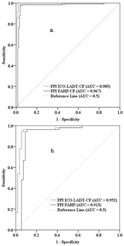
In this work, the vulnerability to flooding in the Prahova River basin was calculated and analyzed using advanced methods and techniques. Thus, 2 hybrid models represented by Iterative Classifier Optimizer – Multiclass Alternating Decision Tree – Certainty Factor (ICO-LADT-CF) and Fuzzy-Analytical Hierarchy Process – Certainty Factor (FAHP-CF) were generated, which had as input data the values of 10 flood predictors and a number of 158 points where historical floods occurred. In the first step, the Certainty Factor values were calculated, which were then used in the Fuzzy-Analytical Hierarchy Process and Multiclass Alternating Decision Tree models. It should be mentioned that the Multiclass Alternating Decision Tree model was optimized with the help of the Iterative Classifier Optimizer. In the case of both ensemble models the slope angle was the most important flood conditioning factor. Moreover, according to Certainty Factor modelling the 8 classes/categories achieved the maximum value of 1. Next, the susceptibility to floods on the surface of the study area was derived. On average, about 20% of the study area has areas with high and medium susceptibility to flash floods. After evaluating the quality of the models through Receiver Operating Characteristics (ROC) Curve, the following results emerged: Success Rate for Flood Potential Index (FPI) Iterative Classifier Optimizer – Multiclass Alternating Decision Tree – Certainty Factor (ICO-LADT-CF) (Area Under Curve = 0.985) and Flood Potential Index (FPI) Fuzzy-Analytical Hierarchy Process – Certainty Factor (FAHP-CF) (Area Under Curve = 0.967); Prediction Rate for Flood Potential Index (FPI) Iterative Classifier Optimizer – Multiclass Alternating Decision Tree – Certainty Factor (ICO-LADT-CF) (Area Under Curve = 0.952) and Flood Potential Index Fuzzy-Analytical Hierarchy Process – Certainty Factor (FAHP-CF) (Area Under Curve = 0.913). At the same time, the accuracies of the models were: Training dataset − 0.943 (Iterative Classifier Optimizer – Multiclass Alternating Decision Tree – Certainty Factor) and 0.931 (Fuzzy-Analytical Hierarchy Process – Certainty Factor); Validating dataset − 0.935 (Iterative Classifier Optimizer – Multiclass Alternating Decision Tree – Certainty Factor) and 0.926 (Fuzzy-Analytical Hierarchy Process – Certainty Factor). As main conclusion, it can be mentioned that the 2 ensemble models outperform the previous machine learning models applied on the same study area before.

Keywords:

• Prahova river basin
• machine learning
• hybrid models
• flood susceptibility
• risk assessment

1. Introduction

As a natural hazard, floods can pose a major problem to communities in the event that they do not have geospatial planning (Uddin and Matin 2021). It is widely acknowledged that geospatial technology can eliminate flood disaster risks and promote decision-making when it comes to flood management (Zhou et al. 2021a). There have been many attempts to reduce flood damage over the past few decades by examining floods, creating flood hazard maps, and analyzing floods in order to minimize flood damage (Rojas et al. 2022; Zhou et al.2021b). It has been unanimously acknowledged by many scientists that hazard zoning has an important role to play in the spatial planning processes (Ma et al. 2023). There are two kinds of flooding: fluvial flooding, which occurs when an increase in the water level of a stream or river overflows into its surrounding area and subsequently into the coastal area, and pluvial flooding, which occurs when excessive runoff from rainfall causes a rapid rise of water levels (Ho et al. 2022; Zhou et al. 2021c). It’s possible that a significant increase in water levels may have been caused by excessive rain, snowmelt, or a combination of both (Tian et al. 2019). In addition to causing property and life losses, snowmelt floods are often associated with numerous flood events. Increasing flood preparedness requires a better understanding of the hydrology of cold regions and how snowmelt causes flooding (Venegas-Cordero et al. 2023; Tian et al. 2020). A cold area is represented also by the upper part of Prahova River catchment from Romania. Over the period of 1950 to 2005, there were a total of around 40% of deaths in Europe attributed to flooding that occurred due to flash floods (Yao et al. 2022). It has become more and more prevalent to emphasize the prevention and mitigation of floods in order to reduce the damage of life and property that can be caused by devastating hazards upon occurrence due to our limited ability to save lives and properties (Li et al. 2018; Yin et al. 2023a). In order to take the most appropriate measures to mitigate the negative effects of flood phenomena, an accurate risk analysis should be done.

A flood risk analysis includes flood hazard mapping as part of the process, which provides an efficient and accurate means to determine the spatial extent of flood characteristics such as velocity, depth, and frequency at the time of an event (Parizi et al. 2022; Zhao et al. 2020; Gao et al. 2021). Maps of flood hazards play an important role in flood management strategies because they show what flood hazard is in a specific location. Over the past few years, a lot of research has been conducted on the analysis, prediction, and quantification of floods and their effects on the Earth (Fekete 2019; Li et al. 2022). One of the approaches include the application of multicriteria decision-making analysis like Analytical Hierarchy Process, TOPSIS, VIKOR (Dahri and Abida 2017; Xie et al. 2021). Another type of techniques include bivariate statistical analysis such as Frequency Ratio, Weights of Evidence, Index of Entropy or Certainty Factor (Cao et al. 2020). Because these approaches usually rely on expert knowledge and are frequently subject to bias and uncertainty, the results often lead to inaccurate conclusions. Simulation of hydrological processes using hydrodynamic models enables hydrological models to identify the relationships between the floods and their predictors. As a result, it is difficult to develop models that are accurate and based on long-term topographic, hydrological, and meteorological data, which can be difficult to acquire. In addition to this, hydrological models tend to be site-specific and are generally not suitable for large-scale regional studies, because their use within other river basins is very limited, as they are often site-specific (Yao et al. 2022). Modeling of flash floods has become increasingly more sophisticated thanks to advancements in the use of high-performance computing technique and machine learning (ML) approaches. These can be described as a data-driven method, where a data-driven model takes into account the training data and the influencing factors so as to establish a quantitative model that can predict flood susceptibility by analyzing the relationship between flood occurrence and these factors. The most representative machine learning models include: logistic regression (Ali et al. 2020), support vector machine (Costache 2019), artificial neural networks (Chapi et al. 2017), naïve bayes (Chen et al. 2020) or random forest (Lee et al. 2017). Though, it is considered that the accuracy of stand-alone machine learning techniques can be exceeded by the ensemble machine learning models (Li and Hong 2023; Yin et al. 2023a). Therefore, in the last period of time many ensembles of hybrid models were applied in order to solve the issue of model’s accuracy. Thus, the most well-known ensembles are boosting, AdaBoost or stacking based models (Luu et al. 2021). Nevertheless, there is no general consensus regarding the most accurate or performant machine learning based ensemble that could be applied in order to estimate the flood susceptibility.

Therefore, the primary objective of this paper is to explore the impact of coupling a bivariate statistics model and fuzzy multicriteria decision-making analysis with a novel decision tree model. The resulted machine learning model (LADT-CF) will be optimized with Iterative Classifier Optimizer (ICO) technique. Additionally, the next specific objectives of this work can be mentioned: i) inventory of flood points; ii) collection and description of flood predictors; iii) computing and applying the ensemble models for Flood Potential Index; iv) spatial representation and validating the results. In this regard, a significant point to note is that in the present study, the accuracy of the model will be evaluated by using ROC curves and several statistics to validate the results of the analysis. The present analysis will be focused on the middle and upper zone of Prahova River. The area has been subject to severe floods in 1970, 1975, 2005, and 2010. Therefore, from practical point of view, it is imperative to highlight these areas as accurately as possible for adequate flood risk management (Avand et al. 2022). In areas that have shown to have a high and very high flood potential, detailed studies can be conducted using hydraulic modeling (Kuriqi and Ardiçlioǧlu 2018) in order to reduce the potential damage (Kuriqi and Hysa 2021).

Using two hybrid models for the first time to determine flood susceptibility is the main novelty of this paper. Moreover, the present results are more accurate than those obtained in previous studies on the same topic.

2. Study area – Prahova basin Romania

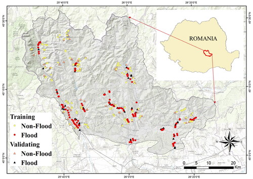
The study area extends over the hill and mountain area in the central-southern part of Romania and occupies an area of about 2600 square kilometers (Figure 1). The elevations of the relief in the study area start from 128 meters in the low hill area, and reach over 2500 m in the high mountain area. In the research area of the study, the flood occurrence is influenced by low slope values arising from the main river valleys and depressions that make up the research area.

Figure 1. Study area location.

The peak of the floods season generated by flash-floods usually occurs between May and July when Cumulonimbus clouds produce torrential rains with extremely high levels of velocity. During this period, the study area receives approximately 15% of the annual amount of rainfall. It can be concluded from the data that out of the two hydrological soil groups B and C, hydrological soil group B dominates in the study area (40% of the total). The vulnerability of the study area to flood phenomena is provided also by the presence of human objectives like 12 cities in which there exists a number of 152506 inhabitants (Costache 2019).

3. Data

3.1. Flood inventory

It is essential to have an in-depth understanding of the areas of previous flooding that are related to flood susceptibility in order to make a highly accurate prediction. It was necessary to conduct an inventory of locations affected by floods in the past to get a better understanding of how some geographical factors can influence flooding. Data was gathered from the archives of the General Inspectorate for Emergency Situations. There were 158 flood events that were detected and mapped in the upper and middle segments of the catchment of the Prahova River in the upper and middle sectors of the catchment. 158 additional non-flooded points have been included in the present study in order to enhance the objectivity of the results obtained as a result of this study. The areas that were not affected by floods were randomly selected from the interfluvial zones, or in areas with very steep slopes, which would make it nearly impossible for floods to occur. Flood-affected points have been assigned the value of 0, while non-affected points have been assigned the value of 1. A percentage of 70% of floods is categorized as training dataset (110 – flood points, 110 - non-flood points), while the rest of 30% was kept as validation dataset (48 – flood points, 48 – non-flood points).

3.2. Flood predictors

In order to accurately determine flood susceptibility values, it is crucial to consider geographic factors that best explain the flooding process. This study used 10 geographic factors to identify flood-prone areas: elevation, plan curvature, slope angle, distance from rivers, lithology, topographic wetness index, hydrological soil group, land use, rainfall, and convergence index in order to identify flood-prone areas.

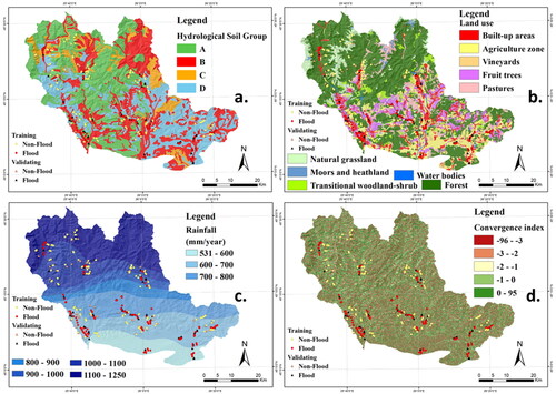
Among the factors that affect natural hazards analyses, elevation is one of the most important. Flooding is virtually impossible at high elevations, but flat areas are highly susceptible. According to Chen et al. (2020), flowing water from hillsides connects to lower regions of rivers, causing flooding. It is important to consider the effect of elevation on runoff amount and velocity. The importance of elevation factor is given by its usage in the many previous studies related to the flood susceptibility evaluation (Arabameri et al. 2020; Luu et al. 2021; Li et al. 2022; Yao et al. 2022; Zhuo et al. 2022). In our case, the study area is divided into eight elevation classes, with those between 200 m and 400 m accounting for the largest spatial extension (25%), followed by those between 400 m and 600 m (Figure 2a). It is important to keep in mind that plan curvature is also one of the influencing factors in flood studies (Ali et al. 2020). According to the literature (Akay 2021), this factor is often categorized into three categories: flat, convex, and concave (Figure 2b). The influence of this morphometric predictor in flood genesis is acknowledged by many authors in the literature (Chapi et al. 2017; Chowdhuri et al. 2020; Zhu et al. 2022). In order to calculate the slope, we use the angle between the horizontal datum and the ground as the reference. Essentially, it is concerned with the effect of gravity on the creation and velocity of runoff, as well as its quality (Bui et al. 2020; Cao et al. 2020; Rui et al. 2023). In fact, this conditioning factor has a great deal of importance for hydrological analysis as a result. Due to the increased volume of water that reaches rivers as a consequence, floods are triggered (Figure 2c). Around 40% of the research zone have slopes ranging in intensity from seven to fifteen degrees. Distance from river represents a critical geographical factor due to the fact that most of the flood phenomena are triggered by high rivers discharges (Saleh et al. 2022). According to the literature (Abdulrazzak et al. 2019), the distance from river factor was computed using the Euclidean distance tool having as basis the river network in shapefile format (Figure 2d). The number of floods decreasing with increasing distance from the hydrographic network is remarkable, with over 40% of flood events occurring within 50 meters of rivers. Another important factor derived from vectorial database is represented by lithology. This factor has a very high influence in terms of water infiltration process (Yang et al. 2018; Xu et al. 2022). Thus, in the case of rocks with a high impermeability and hydraulic conductivity, the flood phenomena will have a higher probability to occur, that the areas characterized by the presence of rocks with a higher permeability (Li et al. 2021). In this study, the lithological groups were extracted from the Geological Map of Romania, 1:200.000 (Figure 2e). The topographic wetness index (twi) (Figure 2f) is a morphometrical factor calculated using the relationship between slope and catchment area (Azareh et al. 2021). High values of twi factor are directly related to the areas where the probability of flooding is considerably higher. The range of values is between 8.5 and 12, the middle class having the highest percentage of flood pixels equal to 30%. The hydrological soil groups (Figure 3a) are a factor that has a strong relation with the flood conditions. The hydrological groups are mainly established according to their texture (Stewart et al. 2012). Infiltration of water is enhanced by coarser textures and stoniness, which are associated with larger pores (Xu et al. 2021; Golkarian et al. 2023; Sun et al. 2023). In the study area the main hydrological soil group is C (68%). According to Zhao et al. (2023), land use is another significant factor that plays a significant role in the occurrence of floods. Flood occurrence and vegetation density have generally been found to be negatively correlated (Marino et al. 2023; Yin et al. 2023b). The forest is present on approximately 50% of the study zone, while the most flood pixels are located in the built-up areas. Compared to the timing of rain on vegetated lands, the speed of rain on non-vegetated lands is much faster than in vegetated or planted areas (Figure 3b). Thus, the areas covered by impervious surfaces, such as concrete, concrete structures, and impervious surfaces, tend to flood more frequently than the regions with plantations and trees (Al-Taani et al. 2023). Flooding is caused directly by rainfall (Figure 3c), according to a large number of existing studies (Wu et al. 2023). Due to this, flood susceptibility maps consider it to be one of the most important factors (Tariq et al. 2023). Convergence index is a morphometric measure whose values have a big influence in the flood occurrence process (Costache and Bui 2019). Their values close to 100 are characteristics for zones with a lower flood susceptibility while the values close to −100 represent the areas with a high flood susceptibility (Figure 3d).

Figure 2. Flood conditioning factors (a. Elevation; b. Plan curvature; c. Slope angle; d. Distance from river; e. Lithology; f. TWI).

Figure 3. Flood conditioning factors (a. Hydrological soil group; b. Land use; c. Rainfall; d. Convergence index).

4. Methods

4.1. Relief-F method

The Relief-F algorithm employs an iterative process for adjusting feature weights in order to distinguish between neighboring patterns based on the dimensions of the features. As an example, let us assume mathematically that x is a random sample of binary class data that has been randomly selected (Tuncer et al. 2020). An estimate can be made of two neighbours of a given object, where one can represent the nearest neighbor in terms of class (called a nearest hit or NH) and the other can represent its nearest neighbour in terms of class (called a nearest miss or NM). The estimation of ReliefF coefficients values can be done using the next mathematical relations (Tuncer et al. 2020): (1) $$w_i\leftarrow w_i+\left|x^{\left(i\right)}+{\mathrm{NM}}^2\right|-\left|x^{\left(i\right)}-{\mathrm{NH}}^2\right|$$(1) where w is the weight for the i-th feature; NM is the nearest miss; NH is the nearest hit; x is a randomly selected sample from a binary class data.

4.2. Certainty Factor (CF)

For the mapping of natural hazard susceptibility, the certainty factor approach has become one of the commonly used approaches for determining the level of probability of a given event as a result of combining heterogeneous data (Wang et al. 2019). As a result, it will be necessary to calculate the value of the Certainty Factor by applying the following equation to each class/category of flood predictors (Wang et al. 2019): (2) $$CF=\{\begin{array}{c}\frac{{PP}_a-{PP}_s}{{PP}_a{(1-PP}_s)},\mathit{\text{ if }}{PP}_a\ge {PP}_s\\ \frac{{PP}_a-{PP}_s}{{PP}_s{(1-PP}_a)},\mathit{\text{ if }}{PP}_a<{PP}_s\end{array},$$(2)

In a study area of a certain size, PPa represents the conditional likelihood of flood pixels occurring in class a, whereas PPs represents the prior probability of flood pixels occurring in the entire study area of a certain size.

Further, the conditional probability (PP_a) values will be determined (Costache 2019): (3) $$\mathit{PPa}\mathrm{ }=\mathrm{ }P\left\{S|B\right\}=\frac{P\left\{S\cap B\right\}}{P\left\{B\right\}}=\frac{\mathit{Npix}\left\{S\cap B\right\}}{\mathit{Npix}\left\{B\right\}},$$(3) where P{S|B} stands for the conditional probability that a flood to occur in the unit B; Npix{S∩B} represent the total amount of flood pixels located in class B; Npix{B} is the amount of pixels from class B.

To calculate prior probabilities (PPs), divide the number of pixels within the study area representing flood phenomena by the number of pixels inside the study area. To this end, the next mathematical expression will be involved (Costache 2019): (4) $$\mathit{PPs}\mathrm{ }=\mathrm{ }P\left\{S\right\}=\frac{\mathit{Npix}\left(\mathit{flood}\right)}{\mathit{Npix}\left(\mathit{total}\right)},$$(4) where P{S} represents the value of the prior probability, Npix(flood) – represents the amount of pixels having flood phenomena in the study region; Npix(total) – represents the total pixels from study region.

4.3. Fuzzy-AHP

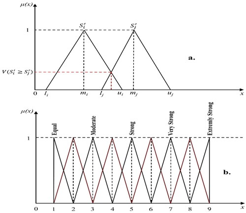
The fuzzy AHP modeling will be involved in the present research paper to estimate the flood susceptibility. Thus, the study extent method using triangular fuzzy numbers (TFN) will be used to derive the fuzzy weights of the flood predictors. Initially, the AHP method is applied based on a literature survey and expert opinion specific to the area of study, and it is the first step in the development of the research report. It is then developed a judgment matrix based on pairwise comparisons, and decision-makers/experts are invited to fill in the judgment matrix with their views. In order to compare the prominence of the elements in the matrix, eigenvalues and eigenvectors were calculated to be able to examine their consistency. Afterward, the matrix judgments are checked to ensure that they are consistent with the pairwise evaluations that follow. In the event of a failure of the consistency test, it is necessary for the original values of the pairwise comparison matrix to be revised. There is a second stage of fuzzy logic used in decision-making where the fuzzy membership function (MF) is determined by looking at the spatial relationships of the conditioning factors to determine the fuzzy membership function (MF) (Ayyildiz and Taskin Gumus 2021). An object can be given a membership value in the fuzzy set theory that ranges between 0 and 1, indicating the degree to which the object belongs to the fuzzy set theory. During Step-1 above, the pairwise comparison scores are transformed into linguistic variables, which are then used to assess alternative scenarios under a fuzzy environment, according to Chang’s fuzzy AHP theory (Tripathi et al. 2022). In order to achieve this, all flood conditioning factors have been converted into one of the following ranges: 0 (low susceptible) to 1 (high susceptible). The synthetic extent values were derived using the next formula (Costache et al. 2022): (5) $$S_i^{\prime }=\sum _j^n{a}_{ij}^{\prime }\mathrm{ }⨂{\left[\sum _{k=1}^n\sum _{j=1}^n{a}_{kj}^{\prime }\right]}^{-1}=\left(\frac{\sum _{j=1}^n{l}_{ij}}{\sum _{k=1}^n\sum _{j=1}^n{u}_{kj}},\frac{\sum _{j=1}^n{m}_{ij}}{\sum _{k=1}^n\sum _{j=1}^n{m}_{kj}},\frac{\sum _{j=1}^n{u}_{ij}}{\sum _{k=1}^n\sum _{j=1}^n{l}_{kj}}\right),\mathrm{ }i=1,\dots ,n.\mathrm{ }$$(5)

The computation of the degree of possibility of $S_i^{\prime }$≥ $S_j^{\prime }$ (Figure 4) represents the third step and is being achieved through the following formula (Costache et al. 2022): (6) $${V(S_i^{\prime }\ge S}_j^{\prime })=\{\begin{array}{l}1,\mathrm{ \hspace{0.17em}}if m_i{\ge m}_j,\\ \frac{u_i{\text{-}\mathrm{ }l}_j}{{(u}_i{\text{-}\mathrm{ }m}_i)+{(m}_j{\text{-}\mathrm{ }l}_j)\mathrm{ }}, l_j{\le \mathrm{ }u}_i, i,j=1, \dots , n;j\ne i \\ 0, \mathit{others}\end{array}$$(6) where $S_i^{\prime }=(l,m_i,u_i)$ and $S_j^{\prime }=(l_j,m_j,u_j).$

Figure 4. a. The degree of possibility of ${\mathrm{S}}_{\mathrm{i}}^{\prime }$≥ ${\mathrm{S}}_{\mathrm{j}}^{\prime };$ b. Triangular fuzzy number corresponding to linguistic variables according to the level of preference.

Considering that (Costache et al. 2022): (7) $$w^{\prime }\left(a_i\right)=\min \hspace{0.17em}\{{V(S_i^{\prime }\ge S}_k^{\prime }\left)\right\},\mathit{ k }=\mathrm{ }1,\mathrm{ }2,\mathrm{ }\dots .,\mathrm{ }\mathrm{n};\mathit{ k }\ne \mathrm{ }\mathrm{i}$$(7)

Then, the value of weight vector will be calculated as: (8) $$w^{\prime }\left(a_i\right)={\left[w^{\prime }\left(a_i\right),\mathrm{ }{w}^{\prime }\left(a_i\right),\mathrm{ }\dots ,\mathrm{ }{w}^{\prime }\left(a_i\right)\right]}^T$$(8) where A_i (i = 1, 2, …, n) are n elements. After the normalization process, the weight vectors can be obtained using the following relation: (9) $$w\left(a_i\right)={\left[w\left(a_1\right),\mathrm{ }w\left(a_2\right),\mathrm{ }\dots ,\mathrm{ }w\left(a_n\right)\right]}^T$$(9) where w is a non-fuzzy number.

AHP weights were applied to each class of factors in ArcGIS 10.5. As a second step, Microsoft Excel 2013 was involved to construct the Fuzzy Analytical Hierarchy Process evaluation matrix associated to the class/category of each factor. Then it was utilized to compute the weights of each predictor in ArcGIS 10.5. To calculate flood susceptibility indexes using the FAHP model, we multiplied the predictors raster in ArcGIS 10.5 and the weights derived through AHP model. Then we applied those weights to the raster using the AHP model.

4.4. Multiclass alternating decision tree (LADTree)

As a result of stretching the alternating decision tree (ADT) model, we can form the LADTree algorithm that can effectively be used for multiclass allocation (Zhao et al. 2022). To separate the original problem into several subproblems, the LogitBoost measure is made use of in conjunction with the ADT model and it is applied to the multiclass alternating decision tree (LADTree) algorithm (Jiroušek and Shenoy 2016). With ADT, decision trees and boosting are effectively combined to yield an effective categorization method that is good at predicting the future and allows for explanation of the results (Holmes et al. 2002). This method is based on polynomial likelihood computations and can be applied directly to multiclass problems by using the LogitBoost method. Taking into account both the LogitBoost method as well as the induction of the LADTree model, we will be able to examine the association between these two methods. As an alternative to the conventional LT1PC model, which generates separate trees for each category in parallel, the second method utilises a more scientifically based approach. LT, on the other hand, requires that only one tree be constructed in order to predict the probability for all classes at the same time. As illustrated in the following formula, two types of symmetric logarithmic conversion are engendered during the computation of the prediction probability for each category in this algorithm (Holmes et al. 2002): (10) $$P_j\left(\mathrm{t}\right)=\frac{e^{Z_j\left(t\right)}}{\sum _{k=1}^N{e}^{Z_k\left(t\right)}},\sum _{k=1}^N{Z}_k\left(t\right)=0\mathrm{ }$$(10) where Z_k(t) represents the function associated to the regression of input variable t after N enhancement sequence are completed. Moreover, it should be noted that Z_k(t) is the sum of the responses of all the ensemble classifier on instance t over N classes.

4.5. Iterative Classifier Optimizer (ICO)

In the case of iterative classifier optimizer (ICO), cross-validation is used and an algorithm is developed that optimizes the number of iterations for a given classifier. It can handle missing, numerical, binary and empty classes as well as attributes such as numeric, nominal and binary (Khosravi et al. 2021). By using the ICO algorithm, a model is developed, and then when the observed and measured values are compared, the model is optimized and, then, after the model performance is examined, the obtained information is introduced to the model for tuning the outputs using the information obtained in the optimization procedure (Saad 2018). In order to increase the accuracy of the prediction, the hybridization is primarily intended to improve the accuracy of the LADTree-CF algorithm by combining them. In this paper, the three aforementioned models have been integrated with the ICO algorithm to improve their outcomes.

4.6. Results validation

Based on the derived flood susceptibility maps of the study, flood points were used to validate the accuracy of the maps. For the purpose of evaluating the performance of the four algorithms used, the AUC-ROC method was adopted (Fang et al. 2021; Yin et al. 2023b). In order to produce an AUC graph, we calculated the sensitivity as well as the 1-specificity. Along with AUC-ROC, the next performance metrics were also used to estimate the results reliability: Sensitivity, Specificity, Accuracy and K-index (Huang et al. 2020; Mi et al. 2023).

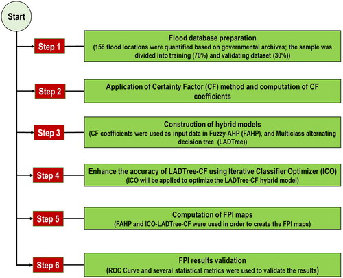
Figure 5 presents in a schematically manner the implemented methodological workflow.

Figure 5. The scheme of the implemented workflow in the present manuscript.

5. Results

5.1. Feature selection

The first step of the implemented workflow consisted in the feature selection procedure. This procedure was applied with the help of ReliefF method. According to the results provided by this method the highest score was assigned to Slope angle (0.134), followed by Distance from rivers (0.127), Elevation (0.114), Land use (0.107), Rainfall (0.1), Hydrological Soil Group (0.094), TWI (0.087), Plan curvature (0.084), Convergence index (0.08) and Lithology (0.074) (Figure 6).

Figure 6. ReliefF score assigned to each flood predictor.

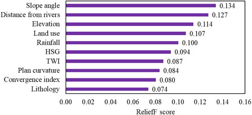
Taking into account the results achieved by each flood conditioning factor, it can be stated that all the variables have an influence related to the flood phenomena. Therefore, all flood predictors will be involved in the modelling procedure.

5.2. Certainty factor

The certainty factor coefficients were calculated for each class associated to the flood conditioning factors using the Microsoft Excel software. The highest value was equal to 1 and have been assigned to the next 8 classes/categories of flood predictors: slope angle lower than 3°; slope angle between 3° and 7°; hydrological soil group A; TWI values between 15.1 and 25; water bodies land use category; elevation class between 128 m and 200 m; distance from river class lower than 50 m; and distance from river class between 50 m and 100 m (Table 1). Thus, the enumerated classes/categories, are, from the CF coefficients point of view, the most favourable to the occurrence of flood phenomenon. In the same time, the lowest value of CF coefficients was equal to −1 and was assigned to a number of 18 classes/categories of flood predictors. Within these classes/categories the flood pixels are not present.

Table 1. CF values for each class/category of flood conditioning factors.

Factor	Class	Class pixels (%)	PPa	CF
Lithology	1	27.28	0.13	−0.85
	2	3.08	0.18	−0.78
	3	0.65	0.00	−1.00
	4	1.43	0.00	−1.00
	5	0.10	0.00	−1.00
	6	0.05	0.00	−1.00
	7	0.89	0.33	−0.50
	8	28.62	0.05	−0.94
	9	14.30	0.32	−0.53
	10	23.45	0.87	0.84
	11	0.07	0.00	−1.00
	12	0.08	0.00	−1.00
Slope	< 3°	11.46	1.00	1.00
	3 - 7°	13.32	1.00	1.00
	7 - 15°	41.72	0.00	−1.00
	15 - 25°	26.42	0.00	−1.00
	> 25°	7.09	0.00	−1.00
Plan curvature	−11.8 − 0	32.68	0.44	−0.23
	0.1 − 0.5	56.65	0.59	0.30
	0.6 − 8.5	10.66	0.00	−1.00
HGS	A	1.52	1.00	1.00
	B	44.41	0.19	−0.76
	C	37.82	0.60	0.33
	D	16.25	0.41	−0.31
TWI	−9.7 − 4.5	21.30	0.41	−0.30
	4.6 − 8.4	24.98	0.38	−0.40
	8.5 - 12	29.70	0.46	−0.16
	12.1 - 15	21.09	0.61	0.35
	15.1 - 25	2.93	1.00	1.00
Land use	Built-up areas	8.61	0.97	0.97
	Agriculture zone	11.55	0.69	0.54
	Vineyards	0.95	0.50	−0.01
	Fruit trees	9.17	0.80	0.75
	Pastures	6.11	0.22	−0.72
	Forest	52.23	0.00	−1.00
	Natural grassland	6.66	0.40	−0.34
	Moors and heatland	0.81	0.00	−1.00
	Woodland-shrub	3.13	0.00	−1.00
	Water bodies	0.78	1.00	1.00
CI	−96 - −3	21.72	0.98	0.98
	−3 - −2	6.34	0.76	0.68
	−2 - −1	8.51	0.11	−0.88
	−1 − 0	10.62	0.00	−1.00
	0 - 95	52.81	0.00	−1.00
Elevation	128 - 200 m	2.12	1.00	1.00
	200 - 400 m	23.38	0.67	0.51
	400 - 600 m	20.96	0.55	0.18
	600 - 800 m	10.42	0.24	−0.69
	800 − 1000 m	11.96	0.50	−0.01
	1000 − 1200 m	12.72	0.00	−1.00
	1200 − 1400 m	10.33	0.00	−1.00
	> 1400 m	8.12	0.00	−1.00
Distance from river	0 - 50 m	4.58	1.00	1.00
	50 - 100 m	4.24	1.00	1.00
	100 − 150 m	4.20	0.92	0.92
	150 - 200 m	3.10	0.92	0.91
	200 - 400 m	14.49	0.20	−0.76
	400 − 700 m	19.64	0.13	−0.85
	700 − 1000 m	16.53	0.09	−0.90
	> 1000 m	33.21	0.03	−0.97
Rainfall (mm/year)	531 - 600 mm	9.94	0.73	0.63
	600 − 700 mm	19.82	0.66	0.47
	700 - 800 mm	16.85	0.52	0.07
	800 - 900 mm	7.34	0.60	0.33
	900 − 1000 mm	5.46	0.45	−0.17
	1000 − 1100 mm	14.61	0.21	−0.74
	1100 − 1250 mm	25.99	0.40	−0.34

Further, in the modelling procedure, the CF coefficients were used as input data in the FAHP and LADTree algorithms.

5.3. FAHP modelling results

The first stage in the computation of FPI with the help of Fuzzy-AHP method, assumes the creation in Microsoft Excel, of a fuzzy pair-wise comparison matrix. In the matrix all the 10 flood conditioning factors were inserted (Table 2). Their importance on flood genesis was the basis for the values assigned when they were compared. The results of the comparison matrix allow us to further compute the equation in which the synthesis values were included (Costache et al. 2022): (11) $${\left[\sum _{k=1}^n\sum _{j=1}^n{a}_{kj}^{\prime }\right]}^{-1}=\mathrm{ }{\left(106.8\mathrm{ }146.8\mathrm{ }193.4\right)}^{-1}=\left(0.0051\mathrm{ }0.0068\mathrm{ }0.0093\right)$$(11)

Table 2. FAHP evaluation matrix.

	1	2	3	4	5	6	7	8	9	10
Altitude (1)
l1	1	1	1	1	2	1/3	3	1	2	2
m1	1	1	1	2	3	1/2	4	2	3	3
u1	1	1	1	3	4	1/1	5	3	4	4
Disntance from river (2)
l2	1	1	1	1	2	1/4	2	1	2	2
m2	1	1	1	2	3	1/3	3	2	3	3
u2	1	1	1	3	4	1/2	4	3	4	4
Land use (3)
l3	1	1	1	1	2	1/3	2	1	3	2
m3	1	1	1	2	3	1/2	3	2	4	3
u3	1	1	1	3	4	1/1	4	3	5	4
HSG (4)
l4	1/3	1/3	1/3	1	1	1/6	1	1	1	1
m4	1/2	1/2	1/2	1	2	1/5	2	1	2	2
u4	1/1	1/1	1/1	1	3	1/4	3	1	3	3
Plan curvature (5)
l5	1/4	1/4	1/4	1/3	1	1/7	1	1/3	1	1
m5	1/3	1/3	1/3	1/2	1	1/6	2	1/2	1	1
u5	1/2	1/2	1/2	1/1	1	1/5	3	1/1	1	1
Slope angle (6)
l6	1	2	1	4	5	1	5	2	4	3
m6	2	3	2	5	6	1	6	3	5	4
u6	3	4	3	6	7	1	7	4	6	5
Convergence index (7)
l7	1/5	1/4	1/4	1/3	1/3	1/7	1	1/3	1	1
m7	1/4	1/3	1/3	1/2	1/2	1/6	1	1/2	1	1
u7	1/3	1/2	1/2	1/1	1/1	1/5	1	1/1	1	1
Lithology (8)
l8	1/3	1/3	1/3	1	1	1/4	1	1	1	2
m8	1/2	1/2	1/2	1	2	1/3	2	1	2	3
u8	1/1	1/1	1/1	1	3	1/2	3	1	3	4
TWI (9)
l9	1/4	1/4	1/5	1/3	1	1/6	1	1/3	1	1
m9	1/3	1/3	1/4	1/2	1	1/5	1	1/2	1	1
u9	1/2	1/2	1/3	1/1	1	1/4	1	1/1	1	1
Rainfall (10)
l10	1/4	1/4	1/4	1/3	1	1/5	1	1/4	1	1
m10	1/3	1/3	1/3	1/2	1	1/4	1	1/3	1	1
u10	1/2	1/2	1/2	1/1	1	1/3	1	1/2	1	1

Results of the previous equations were involved in the computation of fuzzy numbers which will be assigned to each flood predictor. Using the fuzzy numbers, the degree of possibility have been calculated (Table 3). Further, the importance of flood predictor was determined using the next equations: (12) $$w’\left(a_i\right)={\left\{0.\text{49 }0.\text{43 }0.\text{49 }0.0\text{9 }0.0\text{5 1 }0.0\text{3 }0.\text{16 }0.0\text{5 }0.0\text{4}\right\}}^T$$(12) (13) $$w\left(a_i\right)={\left\{0.\text{17 }0.\text{15 }0.\text{171 }0.0\text{31 }0.0\text{17 }0.\text{35 }0.0\text{1 }0.0\text{56 }0.0\text{17 }0.0\text{14}\right\}}^T$$(13)

Table 3. The ordinate of the highest intersection point, the degree possibility for TFNs, and the wright’s landslide predictors.

Altitude = 1	Distance from river = 2	Land use = 3
V(S1 ≥ S2) = 1	V(S2 ≥ S1) = 0.9	V(S3 ≥ S1) = 0.94
V(S1 ≥ S3) = 1	V(S2 ≥ S3) = 0.96	V(S3 ≥ S2) = 1
V(S1 ≥ S4) = 1	V(S2 ≥ S4) = 1	V(S3 ≥ S4) = 1
V(S1 ≥ S5) = 1	V(S2 ≥ S5) = 1	V(S3 ≥ S5) = 1
V(S1 ≥ S6) = 0.49	V(S2 ≥ S6) = 0.43	V(S3 ≥ S6) = 0.49
V(S1 ≥ S7) = 1	V(S2 ≥ S7) = 1	V(S3 ≥ S7) = 1
V(S1 ≥ S8) = 1	V(S2 ≥ S8) = 1	V(S3 ≥ S8) = 1
V(S1 ≥ S9) = 1	V(S2 ≥ S9) = 1	V(S3 ≥ S9) = 1
V(S1 ≥ S10) = 1	V(S2 ≥ S10) = 1	V(S3 ≥ S10) = 1
min{V(S1 ≥ Sk)} = 0.49	min{V(S2 ≥ Sk)} = 0.43	min{V(S3 ≥ Sk)} = 0.49
Weight = 0.171	Weight = 0.15	Weight = 0.172
HSG = 4	Plan curvature = 5	Slope angle = 6
V(S4 ≥ S1) = 0.52	V(S5 ≥ S1) = 0.08	V(S6 ≥ S1) = 1
V(S4 ≥ S2) = 0.64	V(S5 ≥ S2) = 0.21	V(S6 ≥ S2) = 1
V(S4 ≥ S3) = 0.6	V(S5 ≥ S3) = 0.18	V(S6 ≥ S3) = 1
V(S4 ≥ S5) = 1	V(S5 ≥ S4) = 0.59	V(S6 ≥ S4) = 1
V(S4 ≥ S6) = 0.09	V(S5 ≥ S6) = 0.05	V(S6 ≥ S5) = 1
V(S4 ≥ S7) = 1	V(S5 ≥ S7) = 1	V(S6 ≥ S7) = 1
V(S4 ≥ S8) = 0.91	V(S5 ≥ S8) = 0.5	V(S6 ≥ S8) = 1
V(S4 ≥ S9) = 1	V(S5 ≥ S9) = 1	V(S6 ≥ S9) = 1
V(S4 ≥ S10) = 1	V(S5 ≥ S10) = 0.88	V(S6 ≥ S10) = 1
min{V(S4 ≥ Sk)} = 0.09	min{V(S5 ≥ Sk)} = 0.05	min{V(S6 ≥ Sk)} = 1
Weight = 0.031	Weight = 0.017	Weight = 0.35
Convergence index = 7	Lithology = 8	TWI = 9
V(S7 ≥ S1) = 0.04	V(S8 ≥ S1) = 0.61	V(S9 ≥ S1) = 0.09
V(S7 ≥ S2) = 0.03	V(S8 ≥ S2) = 0.71	V(S9 ≥ S2) = 0.1
V(S7 ≥ S3) = 0.05	V(S8 ≥ S3) = 0.68	V(S9 ≥ S3) = 0.05
V(S7 ≥ S4) = 0.44	V(S8 ≥ S4) = 1	V(S9 ≥ S4) = 0.51
V(S7 ≥ S5) = 0.88	V(S8 ≥ S5) = 1	V(S9 ≥ S5) = 0.99
V(S7 ≥ S6) = 0.06	V(S8 ≥ S6) = 0.16	V(S9 ≥ S6) = 0.07
V(S7 ≥ S8) = 0.34	V(S8 ≥ S7) = 1	V(S9 ≥ S7) = 1
V(S7 ≥ S9) = 0.88	V(S8 ≥ S9) = 1	V(S9 ≥ S8) = 0.41
V(S7 ≥ S10) = 0.74	V(S8 ≥ S10) = 1	V(S9 ≥ S10) = 0.85
min{V(S7 ≥ Sk)} = 0.03	min{V(S8 ≥ Sk)} = 0.16	min{V(S9 ≥ Sk)} = 0.05
Weight = 0.01	Weight = 0.056	Weight = 0.017
	Rainfall = 10
	V(S10 ≥ S1) = 0.05
	V(S10 ≥ S2) = 0.2
	V(S10 ≥ S3) = 0.16
	V(S10 ≥ S4) = 0.63
	V(S10 ≥ S5) = 0.84
	V(S10 ≥ S6) = 0.04
	V(S10 ≥ S7) = 1
	V(S10 ≥ S8) = 0.53
	V(S10 ≥ S9) = 0.99
	min{V(S10 ≥ Sk)} = 0.04
	Weight = 0.014

Additionally, the defuzzification procedure permit the TFNs to be converted into crisp weights that are applied to each flood predictor and then multiplied with CF coefficients in order to derive the FPI_FAHP (Figure 7a).

Figure 7. Flood potential index (a. FAHP-CF; b. ICO-LADT-CF).

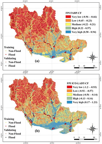
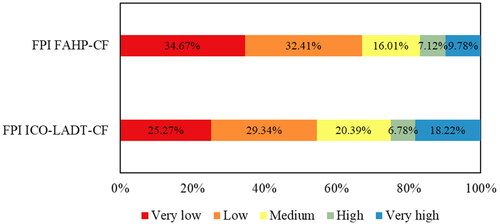
The spatial variation of the FPI_FAHP-CF values ​​was represented in the GIS environment by using cartographic algebra. The derived values ​​of the spatial index fell between −0.96 and 0.94. These were grouped into five classes by the Natural Breaks method. It can be observed that the first class of values, having a very low flood potential, appears mainly in the northern part of the study area, where the relief slope values ​​are very high, and at the same time, the forest cover is very well represented. In these areas, the FPI_FAHP-CF values fall between −0.96 and −0.66 (Figure 7a) and occupy 34.67% of the total study area (Figure 7a). Next, the class of low values is individualized, between −0.65 and −0.23. This class has a weight of 32.41% of the total study area and is present in the median area of the area under research. The average values of flood potential appear in the transition zones between the steep slopes of the hills and the valleys of the main rivers. They fall between −0.22 and 0.21 and occupy a total percentage of 16.01% of the Prahova river basin. The high and very high values of flood potential extend mainly in the southern part of the region under research, where the slopes tend to the 0° value and the forest cover is also missing. It is also noticeable the presence of this potential along the main valleys of the study area. From the point of view of the values, high and very high flood potential is above 0.22 and covers 16.9% of the total studied area.

5.4. LADTree modelling results

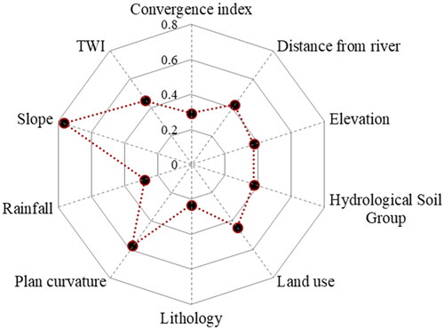
In the case of applying the LADTree-CF algorithm, the ICO helped to determine the best parameters in order to obtain the highest accuracy. The optimization process through the ICO model was made possible by applying a cross-validation method. In the end, accuracy values ​​of 0.967 (for the training sample) and 0.954 (for the validating sample) resulted after a number of 28 iterations applied to the ICO-LADTree-CF hybrid model. Next, the important flood predictors were determined through which the FPI_{ICO-LADTree-CF} was calculated. The highest importance resulted for Slope (0.767), followed by Plan curvature (0.576), TWI (0.451), Land use (0.446), Distance from river (0.421), Elevation (0.377), Hydrological Soil Group (0.376), Convergence index (0.291), Rainfall (0.282) and Lithology (0.232) (Figure 8).

Figure 8. Flood predictors importance in ICO-LADTree-CF model.

In the case of FPI_ICO-LADT-CF, the values were obtained by multiplying the importance of each flood predictor with the CF values. The difference in values fell between −1.2 and 1.23, it being divided into 5 classes by using the same Natural Breaks method as in the situation presented previously. About 25.27% of the total study area is characterized by a very low flood potential. This is associated with the range between −1.2 and −0.93 (Figure 7b). As in the case of the other index, the very low values appear mainly in the northern half of the Prahova river basin, where the slopes have very high values and the degree of afforestation is also very high. The low values of FPI_ICO-LADT-CF between −0.92 and −0.57 have a weight of 29.34% of the total study area, while medium flood potential is located on around 20.39%. The high and very high flood potential is present on 25% of Prahova river basin (Figure 9).

Figure 9. Percentage of each FPI class.

5.5. Results validation

The first method applied to evaluate the accuracy of the obtained results is the ROC Curve. Thus, through the training data set and the FPI values, the Success Rate was built (Fig. xa). As can be seen, the AUC value associated with FPIICO-LADT-CF is 0.985 and exceeds that attributed to FPIFAHP-CF, which was 0.967. And in the case of Prediction Rate for which the validation sample was used together with the flood potential values, the AUC related to FPIICO-LADT-CF was higher than the AUC value for FPIFAHP. Thus, for the first applied model the AUC was 0.952, while for the second model the AUC was equal to 0.913 (Figure 10b).

Figure 10. ROC Curve (a. Success Rate; b. Prediction Rate).

The second group of methods used to evaluate the results is represented by the application of several statistical indicators. In order to calculate these indicators in a first stage, it was necessary to establish the values of the following variables: True Positive (TP), True Negative (TN), False Positive (FP) and False Negative (FN). The use of the training sample showed Sensitivity values of 0.95 for FPI_ICO-LADT-CF and 0.934 for FPI_FAHP-CF. And in the case of Specificity, the value attributed to FPI_ICO-LADT-CF of 0.936 was higher than the one associated with FPI_FAHP-CF, which was 0.927. Accuracy value varied between 0.943 for FPI_ICO-LADT-CF and 0.931 for FPI_FAHP-CF. As expected, the K-index value was also higher in the case of FPI_ICO-LADT-CF (0.886) compared to FPI_FAHP-CF (0.862) (Table 4).

Table 4. Flood potential maps accuracy assessment using statistical metrics.

Metrics	Training sample		Validating sample
	ICO-LADT-CF	FAHP-CF	ICO-LADT-CF	FAHP-CF
TP	115	114	52	49
TN	117	115	49	51
FP	8	9	2	5
FN	6	8	5	3
Sensitivity	0.950	0.934	0.912	0.942
Specificity	0.936	0.927	0.961	0.911
Accuracy	0.943	0.931	0.935	0.926
K-index	0.886	0.862	0.870	0.852

In the case of using the validating sample, the Sensitivity value was higher (0.942) for FPI_FAHP-CF compared to FPI_ICO-LADT-CF (0.912). At the same time, the Specificity value for FPI_ICO-LADT-CF (0.961) exceeds that attributed to FPI_FAHP-CF (0.911). These values ​​once again led to a higher Accuracy for FPI_ICO-LADT-CF (0.935) compared to the one associated with FPI_FAHP-CF (0.926). And the K-index value obtained in the case of FPI_ICO-LADT-CF (0.87) is higher than that obtained in the case of FPI_FAHP-CF (0.852).

6. Discussion

In the real world, many geographical factors play a very important role in the flood phenomenon genesis (Yin et al. 2023c). There are two categories of factors, exogenous and endogenous elements of the world, which contribute to or influence flood susceptibility. It is important to recognize that there are several internal elements of flood occurrence at varying levels, which include geomorphology, soil, geology, and socio-hydrology (Luo et al. 2022a). Physiographic characteristics as well as land use characteristics play a critical role in preventing frequent floods. In the present research the following 10 flood predictors were taken into account: elevation, plan curvature, slope angle, distance from river, lithology, topographic wetness index, hidrological soil group, land use, rainfall and convergence index. In order to verify the contribution of each flood predictor in flood susceptibility process the ReliefF method was applied. Also, if a predictor achieves a score equal to 0, it will be removed from analysis because that means it do not have any influence on flood susceptibility (Ahmadlou et al. 2019). According to the results, the highest importance the most influential factors proved to be the slope angle, distance from river and elevation. This is in agreement with many previous research work carried out in literature (Ahmadlou et al. 2021; Arabameri et al. 2020; Chowdhuri et al. 2020).

In order to achieve high quality results, the data associated to the flood predictors should be used as input in advanced and accurate models. Several studies have been conducted over the past few years across a wide variety of regions around the world using a wide variety of decision-making techniques, approaches, principles, and concepts (Handini et al. 2021; Chen et al. 2023). As a matter of fact, it is relatively new for flood susceptibility modeling to be based on machine learning algorithms and GIS (Popa et al. 2019). In terms of applications involving predictive analytics and making maps more appealing to viewers, machine learning could be used to speed up the processing and interpretation of data. The ML approach used in this study has previously been shown to be an excellent tool for this application, as previously investigated (Bui et al. 2020). In order to manage large datasets with constrained capacity, academics and data scientists need to be able to use machine learning methodologies. There are several machine learning methodologies that can be used to teach academics and data scientists how to manage large datasets with limited bandwidth (Yang et al. 2022; Luo et al. 2022b). Having access to information about likely target areas in a timely manner could potentially provide both lives and property with information that could aid in evacuation. Therefore, as a result of this information and the maps that could be created with it, flooding can potentially be regulated and prevented. In addition, these findings could be used as a basis for developing a value evaluation criterion that could be used to evaluate the value of quantitative data that is used to develop management plans for rivers, land uses and flood protections (Luu et al. 2021). There is also a need to constantly research and develop new models of floods in order to be able to understand the different aspects of floods. In the present research, the flood susceptibility maps were created using two hybrid models represented by FAHP-CF and ICO-LADT-CF. As can be seen, hybrid models were generated from several categories of stand-alone models. Thus, FAHP is part of both the category of fuzzy models and the category of specific multicriteria decision-making analysis models. At the same time, CF is a bivariate statistical method, a category that also includes frequency ratio, weights of evidence or index of entropy. Furthermore, the use of the LADT machine learning decision tree method in the present study is noteworthy. At the same time, it was desired to optimize this machine learning model by using the ICO algorithm. Thus, by generating the 2 hybrid models, the combined use of the capabilities of methods that are part of several categories was desired. The results proved to be very accurate, both models having an AUC greater than 0.913 and an accuracy above 0.926. These values ​​exceed the performances obtained on the same study area by Costache (2019) who applied several models to estimate flood susceptibility including Adaptive Neuro-Fuzzy Inference System (ANFIS), Fuzzy-Support Vector Machine (FSVM) and Statistical Index. These models achieved a maximum AUC of 0.911 (FSVM). Therefore, it can be stated that the present study presents an improvement in the quality and precision of the results compared to the previous one.

One of the advantages of the present study is given by the short time in which accurate results can be obtained regarding the susceptibility to floods for a considerably large area such as the Prahova river basin (approx. 2600 km²). The alternative to such a study is the use of hydraulic modeling, which in the present case would require a very long processing time and the use of much larger data and resources. Thus, the results of the hydraulic modeling for a surface equal to that of the present study would be obtained after a very long period of time.

Like any research work the present study and methodology applied in this study are subject to limitations and possible uncertanties. Thus, one of the limitation of this study and methodology is represented by the impossibility to derive the depth and velocity of river flow during the flood events. These parameters can be assessed using the hydraulic modelling. The uncertainties of data can be brought by the measurements done in the: i) land use/land cover dataset; ii) rainfall dataset; iii) soil dataset; iv) lithological and topographic dataset. These uncertainties are probably to induce some inaccuracies in the susceptibility results. Another element of limitation is represented by the lack of flood historical data. This element is usually used to calibrate and validate the flood susceptibility results.

Nevertheless, the value of such studies for policymakers cannot be overstated. Policymakers have an important role in regulating and decreasing flood vulnerability by developing and implementing flood-resistance policies and regulations. Land use planning policies that direct development away from flood-prone areas, such as floodplains, coastal zones, and other susceptible places, can be implemented by policymakers (Islam et al. 2021). This may involve zoning regulations, construction codes, and development limits in high-risk locations. Floodplain management policies can be established by policymakers to focus on actions such as floodplain mapping, flood zoning, and land acquisition or transfer of properties in flood-prone locations. This can aid in the prevention or reduction of development in flood-prone areas (Saleh et al. 2022).

7. Conclusions

The present work has highlighted an experimental approach through which the susceptibility of mapping floods was computed based on the integration of several models from diverse categories in the Prahova River basin from Romania. All the models were combined into 2 hybrid models (ICO-LADT-CF and FAHP-CF) that have as input data 10 flood conditioning factors and a number of 158 flood and non-flood locations. Through the 2 models, the importance of the 10 predictors was determined in the first phase. These values were then used in ArcGIS to calculate flood susceptibility across the study area. The results highlighted the fact that the Prahova River basin presents a high and very high susceptibility to flooding on a percentage between 16.9% (FPI FAHP-CF) and 25% (FPI ICO-LADT-CF). It is also worth noting that 2 categories of methods (ROC Curve and Statistical Metrics) were used in order to evaluate the accuracy of the models and validate the results. Thus, according to the ROC Curve, ICO-LADT-CF obtained an AUC higher than 0.952, while FAHP-CF obtained an AUC higher than 0.913. Statistical metrics showed an Accuracy of over 0.935 for ICO-LADT-CF and over 0.926 for FAHP-CF.

The main novelty of this research paper is the use for the first time of the 2 hybrid models in order to determine flood susceptibility. It is also worth noting that the present results proved to be more accurate than the results obtained in previous works on the same study area.

As a result of the precise results obtained through the 2 hybrid models, this study will be of major interest for future research works aimed at determining flood susceptibility, both in Romania and in any other area of the globe. Also, the results of this study will be of major interest both for the National Institute of Hydrology and Water Management of Romania, which is responsible for issuing flood warnings, and for the General Inspectorate for Emergency Situations, which is responsible for interventions in the event of disasters natural.

At the global level, there is more and more evidence of the significant influence of climate change in terms of the severity and manifestation of floods and floods. For this reason, in the future studies the authors will incorporate the climate changes characteristics in order to evaluate the flood susceptibility on Prahova River basin from Romania.

Compliance with ethical standards

Disclosure of potential conflicts of interest

Ethical approval

This article does not contain any studies with human participants or animals performed by any of the authors.

Authors contributions

Conceptualization, R.C., H.G.A., A.Pm, S.C.P. and A.R.M.T.I.; methodology, R.C., A.Pm S.C.P. and A.R.M.T.I.; software, R.C., A.Pm S.C.P. and A.R.M.T.I.; validation, R.C.; formal analysis, R.C., A.Pm, S.C.P. and A.R.M.T.I.; investigation, R.C., A.Pm, S.C.P. and A.R.M.T.I.; resources, R.C., A.Pm, H.G.A., S.C.P. and A.R.M.T.I.; data curation, R.C., A.Pm, H.A., J.A.A., A.A.A, S.C.P. and A.R.M.T.I.; writing—original draft preparation, R.C., A.Pm, H.A., S.C.P. and A.R.M.T.I.; writing—review and editing, R.C., A.Pm, J.A.A., A.A.A, H.A., S.C.P. and A.R.M.T.I.; visualization, R.C., A.Pm, J.A.A., S.C.P. and A.R.M.T.I.; supervision, R.C.; project administration, R.C.; funding acquisition, R.C. All authors have read and agreed to the published version of the manuscript.

Abbreviations
ICO	=	Iterative Classifier Optimizer
LADT	=	Multiclass Alternating Decision Tree
CF	=	Certainty Factor
FAHP	=	Fuzzy-Analytical Hierarchy Process
ROC	=	Receiver Operating Characteristics
FPI	=	Flood Potential Index
PPa	=	Conditional Likelihood
PPs	=	Prior Probability
${\mathrm{S}}_{\mathrm{i}}^{\prime }$	=	Synthetic Extent Value
MF	=	Fuzzy Membership Function
TFN	=	Triangular Fuzzy Numbers
${\mathrm{V}({\mathrm{S}}_{\mathrm{i}}^{\prime }\ge \mathrm{S}}_{\mathrm{j}}^{\prime })$	=	Degree of Possibility
$\mathrm{w}\left({\mathrm{a}}_{\mathrm{i}}\right)$	=	Weight Vector
AUC	=	Area Under Curve

Acknowledgements

The authors are thankful to the editors and potential reviewers

Disclosure statement

No potential conflict of interest was reported by the author(s).

Data availability statement

The data will be made available upon request by the first author.

Availability of data

The data that support the findings of this study are available on request from the corresponding author.

References

- Abdulrazzak M, Elfeki A, Kamis A, Kassab M, Alamri N, Chaabani A, Noor K. 2019. Flash flood risk assessment in urban arid environment: case study of Taibah and Islamic universities’ campuses, Medina, Kingdom of Saudi Arabia. Geomatics Nat Hazards Risk. 10(1):780–796. doi: 10.1080/19475705.2018.1545705.
- Ahmadlou M, Al‐Fugara A, Al‐Shabeeb AR, Arora A, Al‐Adamat R, Pham QB, Al‐Ansari N, Linh NTT, Sajedi H. 2021. Flood susceptibility mapping and assessment using a novel deep learning model combining multilayer perceptron and autoencoder neural networks. J Flood Risk Management. 14(1):e12683. doi: 10.1111/jfr3.12683.
- Ahmadlou M, Karimi M, Alizadeh S, Shirzadi A, Parvinnejhad D, Shahabi H, Panahi M. 2019. Flood susceptibility assessment using integration of adaptive network-based fuzzy inference system (ANFIS) and biogeography-based optimization (BBO) and BAT algorithms (BA). Geocarto Int. 34(11):1252–1272. doi: 10.1080/10106049.2018.1474276.
- Akay H. 2021. Flood hazards susceptibility mapping using statistical, fuzzy logic, and MCDM methods. Soft Comput. 25(14):9325–9346. doi: 10.1007/s00500-021-05903-1.
- Ali SA, Parvin F, Pham QB, Vojtek M, Vojteková J, Costache R, Linh NTT, Nguyen HQ, Ahmad A, Ghorbani MA. 2020. GIS-based comparative assessment of flood susceptibility mapping using hybrid multi-criteria decision-making approach, naïve Bayes tree, bivariate statistics and logistic regression: a case of Topľa basin, Slovakia. Ecol Indic. 117:106620. doi: 10.1016/j.ecolind.2020.106620.
- Al-Taani A, Al-Husban Y, Ayan A. 2023. Assessment of potential flash flood hazards. Concerning land use/land cover in Aqaba Governorate, Jordan, using a multi-criteria technique. Egyptian J Remote Sens Space Sci. 26(1):17–24. doi: 10.1016/j.ejrs.2022.12.007.
- Arabameri A, Saha S, Chen W, Roy J, Pradhan B, Bui DT. 2020. Flash flood susceptibility modelling using functional tree and hybrid ensemble techniques. J Hydrol. 587:125007. doi: 10.1016/j.jhydrol.2020.125007.
- Avand M, Kuriqi A, Khazaei M, Ghorbanzadeh O. 2022. DEM resolution effects on machine learning performance for flood probability mapping. J Hydro-Environ Res. 40:1–16. doi: 10.1016/j.jher.2021.10.002.
- Ayyildiz E, Taskin Gumus A. 2021. Pythagorean fuzzy AHP based risk assessment methodology for hazardous material transportation: an application in Istanbul. Environ Sci Pollut Res Int. 28(27):35798–35810. doi: 10.1007/s11356-021-13223-y.
- Azareh A, Rafiei Sardooi E, Choubin B, Barkhori S, Shahdadi A, Adamowski J, Shamshirband S. 2021. Incorporating multi-criteria decision-making and fuzzy-value functions for flood susceptibility assessment. Geocarto Int. 36(20):2345–2365. doi: 10.1080/10106049.2019.1695958.
- Bui DT, Hoang N-D, Martínez-Álvarez F, Ngo P-TT, Hoa PV, Pham TD, Samui P, Costache R. 2020. A novel deep learning neural network approach for predicting flash flood susceptibility: a case study at a high frequency tropical storm area. Sci Total Environ. 701:134413. doi: 10.1016/j.scitotenv.2019.134413.
- Cao Y, Jia H, Xiong J, Cheng W, Li K, Pang Q, Yong Z. 2020. Flash flood susceptibility assessment based on geodetector, certainty factor, and logistic regression analyses in Fujian Province, China. IJGI. 9(12):748. doi: 10.3390/ijgi9120748.
- Chapi K, Singh VP, Shirzadi A, Shahabi H, Bui DT, Pham BT, Khosravi K. 2017. A novel hybrid artificial intelligence approach for flood susceptibility assessment. Environ Modelling & Software. 95:229–245. doi: 10.1016/j.envsoft.2017.06.012.
- Chen W, Liu W, Liang H, Jiang M, Dai Z. 2023. Response of storm surge and M2 tide to typhoon speeds along coastal Zhejiang Province. Ocean Eng. 270:113646.doi: 10.1016/j.oceaneng.2023.113646.
- Chen W, Li Y, Xue W, Shahabi H, Li S, Hong H, Wang X, Bian H, Zhang S, Pradhan B, et al. 2020. Modeling flood susceptibility using data-driven approaches of naïve bayes tree, alternating decision tree, and random forest methods. Sci Total Environ. 701:134979., doi: 10.1016/j.scitotenv.2019.134979.
- Chowdhuri I, Pal SC, Chakrabortty R. 2020. Flood susceptibility mapping by ensemble evidential belief function and binomial logistic regression model on river basin of eastern India. Adv Space Res. 65(5):1466–1489. doi: 10.1016/j.asr.2019.12.003.
- Costache R, Bui DT. 2019. Spatial prediction of flood potential using new ensembles of bivariate statistics and artificial intelligence: a case study at the Putna river catchment of Romania. Sci Total Environ. 691:1098–1118. doi: 10.1016/j.scitotenv.2019.07.197.
- Costache R, Trung Tin T, Arabameri A, Crăciun A, Ajin RS, Costache I, Reza Md. Towfiqul Islam A, Abba SI, Sahana M, Avand M, et al. 2022. Flash-flood hazard using deep learning based on H2O R package and fuzzy-multicriteria decision-making analysis. J Hydrol. 609:127747. doi: 10.1016/j.jhydrol.2022.127747.
- Costache R. 2019. Flood susceptibility assessment by using bivariate statistics and machine learning models-A useful tool for flood risk management. Water Resour Manage. 33(9):3239–3256. doi: 10.1007/s11269-019-02301-z.
- Dahri N, Abida H. 2017. Monte Carlo simulation-aided analytical hierarchy process (AHP) for flood susceptibility mapping in Gabes Basin (southeastern Tunisia). Environ Earth Sci. 76(7):302. doi: 10.1007/s12665-017-6619-4.
- Fang Z, Wang Y, Peng L, Hong H. 2021. A comparative study of heterogeneous ensemble-learning techniques for landslide susceptibility mapping. Int J Geographical Information Sci. 35(2):321–347. doi: 10.1080/13658816.2020.1808897.
- Fekete A. 2019. Critical infrastructure and flood resilience: cascading effects beyond water. Wiley Interdiscip Rev: Water. 6:e1370.
- Gao C, Hao M, Chen J, Gu C. 2021. Simulation and design of joint distribution of rainfall and tide level in Wuchengxiyu Region,China. Urban Clim. 40:101005.doi: 10.1016/j.uclim.2021.101005.
- Golkarian A, Khosravi K, Panahi M, Clague JJ. 2023. Spatial variability of soil water erosion: comparing empirical and intelligent techniques. Geosci Front. 14(1):101456. doi: 10.1016/j.gsf.2022.101456.
- Handini DR, Hidayah E, Halik G. 2021. Flash flood susceptibility mapping at Andungbiru Watershed, East Java using AHP-information weighted method. Geos Ind. 6(2):127–142. doi: 10.19184/geosi.v6i2.24173.
- Ho M, Nathan R, Wasko C, Vogel E, Sharma A. 2022. Projecting changes in flood event runoff coefficients under climate change. J Hydrol. 615:128689. doi: 10.1016/j.jhydrol.2022.128689.
- Holmes G, Pfahringer B, Kirkby R, Frank E, Hall M. 2002. Multiclass alternating decision trees. Presented at the Machine Learning: ECML 2002: 13th European Conference on Machine Learning; August 19–23, 2002; Helsinki, Finland. Proceedings 13, Springer. p. 161–172.
- Huang F, Cao Z, Guo J, Jiang S-H, Li S, Guo Z. 2020. Comparisons of heuristic, general statistical and machine learning models for landslide susceptibility prediction and mapping. Catena. 191:104580. doi: 10.1016/j.catena.2020.104580.
- Islam ARMT, Talukdar S, Mahato S, Kundu S, Eibek KU, Pham QB, Kuriqi A, Linh, NTT. 2021. Flood susceptibility modelling using advanced ensemble machine learning models. Geosci Front. 12(3):101075. doi: 10.1016/j.gsf.2020.09.006.
- Jiroušek R, Shenoy PP. 2016. Entropy of belief functions in the Dempster-Shafer theory: a new perspective. Presented at the Belief Functions: Theory and Applications: 4th International Conference, BELIEF 2016; September 21–23, 2016; Prague, Czech Republic. Proceedings, Springer. p. 3–13.
- Khosravi K, Barzegar R, Golkarian A, Busico G, Cuoco E, Mastrocicco M, Colombani N, Tedesco D, Ntona MM, Kazakis N. 2021. Predictive modeling of selected trace elements in groundwater using hybrid algorithms of iterative classifier optimizer. J Contam Hydrol. 242:103849. doi: 10.1016/j.jconhyd.2021.103849.
- Kuriqi A, Ardiçlioǧlu M. 2018. Investigation of hydraulic regime at middle part of the Loire River in context of floods and low flow events. Pollack Periodica. 13(1):145–156. doi: 10.1556/606.2018.13.1.13.
- Kuriqi A, Hysa A. 2021. Multidimensional aspects of floods: nature-based mitigation measures from basin to river reach scale. In: Nature-based solutions for flood mitigation: environmental and socio-economic aspects. Charm: Springer International Publishing. p. 11–33.
- Lee S, Kim J-C, Jung H-S, Lee MJ, Lee S. 2017. Spatial prediction of flood susceptibility using random-forest and boosted-tree models in Seoul metropolitan city, Korea. Geomatics Nat Hazards Risk. 8(2):1185–1203. doi: 10.1080/19475705.2017.1308971.
- Li W, Zhu J, Fu L, Zhu Q, Xie Y, Hu Y. 2021. An augmented representation method of debris flow scenes to improve public perception. Int J Geogr Inf Sci. 35(8):1521–1544. doi: 10.1080/13658816.2020.1833016.
- Li R, Zhang H, Chen Z, Yu N, Kong W, Li T, Wang E, Wu X, Liu Y. 2022. Denoising method of ground-penetrating radar signal based on independent component analysis with multifractal spectrum. Measurement. 192:110886.doi: 10.1016/j.measurement.2022.110886.
- Li Q, Song D, Yuan C, Nie W. 2022. An image recognition method for the deformation area of open-pit rock slopes under variable rainfall. Measurement. 188:110544.doi: 10.1016/j.measurement.2021.110544.
- Li H, Lei X, Shang Y, Qin T. 2018. Flash flood early warning research in China. Int J Water Resour Dev. 34(3):369–385. doi: 10.1080/07900627.2018.1435409.
- Li Y, Hong H. 2023. Modelling flood susceptibility based on deep learning coupling with ensemble learning models. J Environ Manage. 325(Pt A):116450. doi: 10.1016/j.jenvman.2022.116450.
- Luo J, Wang G, Li G, Pesce G. 2022a. Transport infrastructure connectivity and conflict resolution: a machine learning analysis. Neural Comput Applic. 34(9):6585–6601. doi: 10.1007/s00521-021-06015-5.
- Luo J, Niu F, Lin Z, Liu M, Yin G, Gao Z. 2022b. Abrupt increase in thermokarst lakes on the central Tibetan Plateau over the last 50 years. CATENA. 217:106497.doi: 10.1016/j.catena.2022.106497.
- Luu C, Pham BT, Phong TV, Costache R, Nguyen HD, Amiri M, Bui QD, Nguyen LT, Le HV, Prakash I, et al. 2021. GIS-based ensemble computational models for flood susceptibility prediction in the Quang Binh Province, Vietnam. J Hydrol. 599:126500. doi: 10.1016/j.jhydrol.2021.126500.
- Ma S, Qiu H, Yang D, Wang J, Zhu Y, Tang B, Sun K, Cao M. 2023. Surface multi-hazard effect of underground coal mining. Landslides. 20(1):39–52. doi: 10.1007/s10346-022-01961-0.
- Marino D, Palmieri M, Marucci A, Soraci M, Barone A, Pili S. 2023. Linking flood risk mitigation and food security: an analysis of land-use change in the metropolitan area of Rome. Land. 12(2):366. doi: 10.3390/land12020366.
- Mi C, Liu Y, Zhang Y, Wang J, Feng Y, Zhang Z. 2023. A vision-based displacement measurement system for foundation pit. IEEE Trans Instrum Meas. 72:1–15. doi: 10.1109/TIM.2023.3311069.
- Parizi E, Khojeh S, Hosseini SM, Moghadam YJ. 2022. Application of unmanned aerial vehicle DEM in flood modeling and comparison with global DEMs: case study of Atrak River Basin, Iran. J Environ Manage. 317:115492. doi: 10.1016/j.jenvman.2022.115492.
- Popa MC, Peptenatu D, Drăghici CC, Diaconu DC. 2019. Flood hazard mapping using the flood and flash-flood potential index in the Buzău River catchment, Romania. Water. 11(10):2116. doi: 10.3390/w11102116.
- Rojas O, Soto E, Rojas C, López JJ. 2022. Assessment of the flood mitigation ecosystem service in a coastal wetland and potential impact of future urban development in Chile. Habitat Int. 123:102554. doi: 10.1016/j.habitatint.2022.102554.
- Rui S, Zhou Z, Jostad HP, Wang L, Guo Z. 2023. Numerical prediction of potential 3-dimensional seabed trench profiles considering complex motions of mooring line. Appl Ocean Res. 139:103704.doi: 10.1016/j.apor.2023.103704.
- Saad IA. 2018. An efficient classification algorithms for image retrieval based color and texture features. J Al-Qadisiyah for Computer Sci Mathe. 1042.
- Saleh A, Yuzir A, Sabtu N, Abujayyab SK, Bunmi MR, Pham QB. 2022. Flash flood susceptibility mapping in urban area using genetic algorithm and ensemble method. Geocarto Int. 37(25):10199–10228. doi: 10.1080/10106049.2022.2032394.
- Stewart D, Canfield E, Hawkins R. 2012. Curve number determination methods and uncertainty in hydrologic soil groups from semiarid watershed data. J Hydrol Eng. 17(11):1180–1187. doi: 10.1061/(ASCE)HE.1943-5584.0000452.
- Sun X, Chen Z, Guo K, Fei J, Dong Z, Xiong H. 2023. Geopolymeric flocculation-solidification of tail slurry of shield tunnelling spoil after sand separation. Constr Build Mater. 374:130954.doi: 10.1016/j.conbuildmat.2023.130954.
- Tariq A, Beni LH, Ali S, Adnan S, Hatamleh WA. 2023. An effective geospatial-based flash flood susceptibility assessment with hydrogeomorphic responses on groundwater recharge. Groundwater Sustainable Dev. 23:100998. doi: 10.1016/j.gsd.2023.100998.
- Tian H, Pei J, Huang J, Li X, Wang J, Zhou B, Qin Y, Wang L. 2020. Garlic and winter wheat identification based on active and passive satellite imagery and the google earth engine in northern china. Remote Sens. 12(21):3539.doi: 10.3390/rs12213539.
- Tian H, Huang N, Niu Z, Qin Y, Pei J, Wang J. 2019. Mapping winter crops in china with multi-source satellite imagery and phenology-based algorithm. Remote Sens. 11(7):820.doi: 10.3390/rs11070820.
- Tripathi AK, Agrawal S, Gupta RD. 2022. Comparison of GIS-based AHP and fuzzy AHP methods for hospital site selection: a case study for Prayagraj City, India. GeoJournal. 87(5):3507–3528. doi: 10.1007/s10708-021-10445-y.
- Tuncer T, Dogan S, Ozyurt F. 2020. An automated residual exemplar local binary pattern and iterative ReliefF based COVID-19 detection method using chest X-ray image. Chemometr Intell Lab Syst. 203:104054. doi: 10.1016/j.chemolab.2020.104054.
- Uddin K, Matin MA. 2021. Potential flood hazard zonation and flood shelter suitability mapping for disaster risk mitigation in Bangladesh using geospatial technology. Progress in Disaster Sci. 11:100185. doi: 10.1016/j.pdisas.2021.100185.
- Venegas-Cordero N, Cherrat C, Kundzewicz ZW, Singh J, Piniewski M. 2023. Model-based assessment of flood generation mechanisms over Poland: the roles of precipitation, snowmelt, and soil moisture excess. Sci Total Environ. 891:164626. doi: 10.1016/j.scitotenv.2023.164626.
- Wang Q, Guo Y, Li W, He J, Wu Z. 2019. Predictive modeling of landslide hazards in Wen County, northwestern China based on information value, weights-of-evidence, and certainty factor. Geomatics Nat Hazards Risk. 10(1):820–835. doi: 10.1080/19475705.2018.1549111.
- Wu X, Feng X, Wang Z, Chen Y, Deng Z. 2023. Multi-source precipitation products assessment on drought monitoring across global major river basins. Atmos Res. 295:106982.doi: 10.1016/j.atmosres.2023.106982.
- Xie X, Xie B, Cheng J, Chu Q, Dooling T. 2021. A simple Monte Carlo method for estimating the chance of a cyclone impact. Nat Hazards. 107(3):2573–2582. doi: 10.1007/s11069-021-04505-2.
- Xu J, Lan W, Ren C, Zhou X, Wang S, Yuan J. 2021. Modeling of coupled transfer of water, heat and solute in saline loess considering sodium sulfate crystallization. Cold Reg Sci Technol. 189:103335. doi:10.1016/j.coldregions.2021.103335.
- Xu Z, Li X, Li J, Xue Y, Jiang S, Liu L, Luo Q, Wu K, Zhang N, Feng Y, et al. 2022. Characteristics of source rocks and genetic origins of natural gas in deep formations, gudian depression, songliao basin, NE China. ACS Earth Space Chem. 6(7):1750–1771. doi: 10.1021/acsearthspacechem.2c00065.
- Yang M, Wang H, Hu K, Yin G, Wei Z. 2022. IA-Net$:$ An inception–attention-module-based network for classifying underwater images from others. IEEE J Oceanic Eng. 47(3):704–717. doi: 10.1109/JOE.2021.3126090.
- Yang W, Xu K, Lian J, Ma C, Bin L. 2018. Integrated flood vulnerability assessment approach based on TOPSIS and Shannon entropy methods. Ecol Indic. 89:269–280. doi: 10.1016/j.ecolind.2018.02.015.
- Yao J, Zhang X, Luo W, Liu C, Ren L. 2022. Applications of Stacking/Blending ensemble learning approaches for evaluating flash flood susceptibility. Int J Appl Earth Obs Geoinf. 112:102932. doi: 10.1016/j.jag.2022.102932.
- Yin L, Wang L, Li T, Lu S, Tian J, Yin Z, Li X, Zheng W. 2023a. U-Net-LSTM: Time series-enhanced lake boundary prediction model. Land. 12(10):1859.doi: 10.3390/land12101859.
- Yin L, Wang L, Li J, Lu S, Tian J, Yin Z, Liu S, Zheng W. 2023b. YOLOV4_CSPBi: Enhanced land target detection model. Land. 12(9):1813.doi: 10.3390/land12091813.
- Yin H, Zhang G, Wu Q, Yin S, Soltanian MR, Thanh HV, Dai Z. 2023a. A deep learning-based data-driven approach for predicting mining water inrush from coal seam floor using microseismic monitoring data. IEEE Trans Geosci Remote Sens. 61:1–15. doi: 10.1109/TGRS.2023.3300012.
- Yin H, Wu Q, Yin S, Dong S, Dai Z, Soltanian MR. 2023b. Predicting mine water inrush accidents based on water level anomalies of borehole groups using long short-term memory and isolation forest. J. Hydrol. 616:128813.doi: 10.1016/j.jhydrol.2022.128813.
- Yin L, Wang L, Li T, Lu S, Yin Z, Liu X, Li X, Zheng W. 2023c. U-Net-STN: A novel end-to-end lake boundary prediction model. Land. 12(8):1602.doi: 10.3390/land12081602.
- Zhao M, Zhou Y, Li X, Cheng W, Zhou C, Ma T, Li M, Huang K. 2020. Mapping urban dynamics (1992–2018) in Southeast Asia using consistent nighttime light data from DMSP and VIIRS. Remote Sens Environ 248:111980.doi: 10.1016/j.rse.2020.111980.
- Zhao H, Gu T, Tang J, Gong Z, Zhao P. 2023. Urban flood risk differentiation under land use scenario simulation. Iscience. 26(4):106479. doi: 10.1016/j.isci.2023.106479.
- Zhao Q, Chen W, Peng C, Wang D, Xue W, Bian H. 2022. Modeling landslide susceptibility using an evidential belief function-based multiclass alternating decision tree and logistic model tree. Environ Earth Sci. 81(15):404. doi: 10.1007/s12665-022-10525-3.
- Zhou G, Zhang R, Huang S. 2021a. Generalized buffering algorithm. IEEE Access. 9:27140–27157. doi: 10.1109/ACCESS.2021.3057719.
- Zhou G, Deng R, Zhou X, Long S, Li W, Lin G, Li X. 2021b. Gaussian inflection point selection for liDAR hidden echo signal decomposition. IEEE Geosci Remote Sens Lett. 19:1–5. doi: 10.1109/LGRS.2021.3107438.
- Zhou G, Li W, Zhou X, Tan Y, Lin G, Li X, Deng R. 2021c. An innovative echo detection system with STM32 gated and PMT adjustable gain for airborne LiDAR. Int J Remote Sens. 42(24):9187–9211. doi: 10.1080/01431161.2021.1975844.
- Zhu W, Chen J, Sun Q, Li Z, Tan W, Wei Y. 2022. Reconstructing of high-spatial-resolution three-dimensional electron density by ingesting SAR-derived VTEC into IRI model. IEEE Geosci Remote Sens Lett. 19:1–5. doi: 10.1109/LGRS.2022.3178242.
- Zhuo Z, Du L, Lu X, Chen J, Cao Z. 2022. Smoothed Lv distribution based three-dimensional imaging for spinning space debris. IEEE Trans Geosci Remote Sens. 60:1–13. doi: 10.1109/TGRS.2022.3174677.