Investigating a three-dimensional convolution recognition model for acoustic emission signal analysis during uniaxial compression failure of coal

Abstract

Acoustic emission predicts coal sample failure, vital for early warnings and monitoring. The study emphasizes using acoustic emission to predict coal sample failure patterns and establish a discriminative model for monitoring. It employs a lightweight 3D convolutional model combining DenseNet with Group Convolution (GC) and the "squeeze-and-excitation" (SE) module. Coal samples from Xinglongzhuang Coal Mine underwent uniaxial compression, and a subset of experiments with prominent features was selected. The resulting acoustic emission parameters were then transformed into spatiotemporal image sequences for input to the model. Successfully identifying hazardous coal damage stages, all four network structures (DenseNet, DenseNet + GC, DenseNet + SE, DenseNet + GC + SE) achieved over 98.29% predictive accuracy in verification samples. The model exhibited a recall rate of over 98.02% for high-risk samples, effectively capturing spatiotemporal information. DenseNet + GC + SE showed a probability distribution focusing on different risk levels. By integrating group convolution and SE modules, this model significantly reduced both model and time complexity while preserving precision, enhancing efficiency. It effectively discerns diverse acoustic emission features through group convolution and evaluates their significance using the SE module. Compared to the traditional C3D neural network, this model greatly reduces complexity and time requirements while improving efficiency in distinguishing between various damage stages.

Keywords:

• Rock mechanics
• mining engineering
• acoustic emission
• coal damage identification
• 3D convolution

1. Introduction

Shallow coal resources in China are on the brink of depletion, prompting a transition to deep coal mining. Factors such as high in-situ stress and complex geological environments in the deep sections of mines have led to frequent dynamic disasters. Ensuring the safe and efficient extraction of coal mines, therefore, holds paramount significance in terms of monitoring, prediction, and prevention of coal sample damage and dynamic disasters (Yao 2015). Coal sample is inherently heterogeneous, and when subjected to external forces, stress concentration occurs at its internal defects, leading to fracture and the release of transient high-energy elastic waves that propagate outward, resulting in acoustic emission (Liu et al. 2024). Acoustic emission detection is an efficient and highly applicable non-destructive testing technique widely used in mining, geotechnical, and other related fields (Liu et al. 2020a; Yao 2014). Zhang et al. (2021) based their study on the evolution of acoustic emission signals in sandstone under different high-temperature treatments, aimed to identify critical failure information of the sandstone. Zheng et al. (2021) conducted an in-depth investigation into the evolution of acoustic emission events in rocks under uniaxial compression, constructing a mechanical model of rock damage for the analysis of rock stability and failure prediction. Zhang et al. (2018) utilized the acoustic emission waveform analysis method to study the failure mechanisms of jointed rocks and intact rocks under uniaxial compression, exploring two distinct modes of failure with and without joints. The premonitory response of acoustic emissions within coal sample aids in analyzing the evolution of coal sample instability, making the establishment of predictive models based on acoustic emission precursory information pivotal for the monitoring and early warning of coal sample damage and even dynamic disasters.

Many scholars have proposed various coal sample damage early warning models based on the acoustic emission method. Based on different parameters of acoustic emission, coal sample damage analysis is conducted. Kong et al. (2016) and Qian et al. (2023) demonstrated that the waveform of coal sample fractures contains rich information on physical and mechanical properties and fracture modes. Effective time-frequency analysis methods are necessary to accurately extract waveform features. Song et al. (2023b) studied the primary mechanical responses and acoustic emission behavior of coal samples under multistage compression cyclic loading at different loading and unloading rates, summarizing the effects of damping on energy dissipation and phase shift during rock damage. Li and Li (2017) discussed the influence of strain rate and water on the mechanical properties and acoustic emission characteristics of sandstone under impact loads, aiming to investigate the intrinsic causes of dynamic disasters such as vibration-induced events. Liu et al. (2021a) combined findings from acoustic emission experiments, revealing that the number of shear failure zones in sandstone before the peak strength of failure gradually increases, while after the peak strength, it initially increases and then decreases with burial depth. The cumulative input energy, released elastic energy, and dissipated energy all increase with depth. Dou et al. (2020) analyzed the release mode of rock elastic waves and suggested that it is possible to accurately capture signals generated during the crack process through an acoustic emission monitoring system, which helps to reasonably infer the occurrence of joints or faults in the rock mass. Tang et al. (2022), using acoustic emission monitoring technology, observed the dynamic failure of coal, where the variation of root mean square (RMS) of acoustic emission defines the effective crack initiation time and effective crack initiation pressure. Nikolenko et al. (2020) proposed an ultrasonic depth measurement method using transverse waves based on the acoustic emission approach, concluding that cyclic freezing and thawing lead to crack development in coal, affecting its mechanical and consumptive properties. Cheng (2019) studied the mechanical properties, failure characteristics, damage spatial development, and damage evolution features of rock-like materials with different lengths of cracks under uniaxial compression loading. Chi et al. (2021) derived the vertical stress release of overlying strata and the evolution of shear stress concentration on coal seams with different inclinations, determining the stress-driven dynamic evolution of overlying strata structure through numerical simulation, rock mechanics experiments, acoustic emission, and field measurements.

In addition, a plethora of research has emerged predicting coal sample damage based on features such as acoustic emission frequency domain and fractals. For example, Xue et al. (2020) analyzed the short-range correlation of acoustic emission scattering signals to construct a clustering model, aiming to quantitatively describe mechanical behavior. Zuo et al. (2019) initially established the theory of surrounding rock stress gradient failure, uniform strength support for deep tunnels, and a hyperbolic motion model similar to overlying strata, proposing underground combined grouting control technology. Bai et al. (2022) suggested that the behavior of rock mass damage and the process of failure are significantly influenced by the stress path of the rock, discussing crack development and damage mechanisms. Song et al. (2023a) applied AE monitoring and micro-CT scanning to determine the fracture mode of coal samples. The study found that the uniaxial compression test of brittle coal exhibited sudden failure caused by large cleavage fracture, while the cyclic fatigue test showed progressive failure of a mixed fracture network. Guo et al. (2023) conducted uniaxial compression tests on high-temperature sandstone under various real-time cooling rates, studying the influence of cooling rates under thermal coupling on the mechanical properties of sandstone and the mechanisms of its failure.

According to the aforementioned research, significant progress has been made in the prediction of coal sample damage using the acoustic emission method. However, the complex and diverse precursor parameters leading to the catastrophe of coal sample damage make it challenging to establish a unified approach. In recent years, with the rapid iteration of computer performance, deep learning has seen rapid development. The combination of artificial neural networks and acoustic emission methods for predicting rock damage has gradually emerged. Qian et al. (2023), based on various physical experiments of coal sample and uniaxial compression, identified high-frequency and uniaxial compression events using waveform characteristic parameters trained by a multilayer perceptron neural network. Di et al. (2021) accurately identified electromagnetic radiation and acoustic emission interference signals using a recurrent neural network, thereby improving the reliability of rock burst monitoring data. Yang et al. (2021) achieved high recognition accuracy in identifying gangue in coal mining faces and coal washing processes using a one-dimensional CNN model for coal sample reflectance spectroscopy data. So far, the research combining acoustic emission and deep learning for coal sample damage prediction is still in its infancy, and it is still necessary to establish a deep learning-based acoustic emission coal sample damage prediction model. Three-dimensional convolution can fit both spatial information of acoustic emission, such as the phenomenon of event clusters and self-similar fractals observed in acoustic emission localization experiments, and temporal characteristics of acoustic emission, such as the change in event counts and amplitudes over time. It is suitable for predicting coal sample damage based on acoustic emission signals.

In summary, this paper proposes the use of a lightweight three-dimensional convolutional prediction model based on the DenseNet framework, integrating deep learning Group Convolution (GC) and the "squeeze-and-excitation" (SE) module from the attention mechanism to fuse spatiotemporal information from acoustic emission. Simultaneously, laboratory research was conducted, collecting acoustic emission damage events, localization, and amplitude parameters during the uniaxial compression process of coal samples from the Yan’zhou district’s Xinglongzhuang coal mine in Jining, Shandong. These parameters were preprocessed into image sequences capable of describing the spatiotemporal evolution of acoustic emission, serving as input samples for the model. The study aims to quantitatively predict the risk level of coal sample damage and the remaining time of coal sample damage. This paper presents a novel approach for identifying uniaxial compression-induced coal sample damage, providing reference for the research on dynamic instability disaster warning in coal sample masses.

2. Overview of basic algorithms

To enable neural networks to integrate spatiotemporal information, the Convolutional 3D Network (C3D) (Tran et al. 2014) emerged. The C3D network has a simple structure and is widely used in the field of deep learning video analysis. Compared to traditional 2D convolutions, it adds a temporal dimension, enabling it to capture not only spatial information but also temporal features (Zhang et al. 2020). However, the high number of network parameters required by C3D results in somewhat inefficient performance. The Pseudo 3D Residual Network (P3D) (Qiu et al. 2017), based on C3D, uses spatial asymmetrical convolutions, decoupling the 3 × 3 × 3 convolution kernel in C3D into two types of convolution kernels, 1 × 3 × 3 and 3 × 1 × 1. The former is used to obtain spatial features, while the latter is used to obtain temporal information. The P3D network effectively reduces the number of parameters but still falls short in meeting the demand for parameter lightness. In addition, the CLDNN (Sainath et al. 2015) integrates two models of spatial and temporal information, using the output of the spatial network as the input of the temporal network. Although it can effectively explore spatiotemporal information, the model is complex, and training is unstable. Therefore, it is crucial to transform the basic structure of the traditional C3D network and construct a three-dimensional convolution recognition model that can unify acoustic emission spatiotemporal information.

In the era of big data, the rational and rapid integration and processing of information have become essential means to improve work efficiency. However, traditional machine learning algorithms often lag behind the increasing pace of data, making it easy to reach performance bottlenecks. To address the drawbacks of overly dense neurons in the backpropagation (BP) neural network and the disruption of relative positional relationships between pixels when inputting images, the convolutional neural network (CNN) emerged to tackle the issues of large parameter volumes in artificial neural networks and the disruption of local image correlations. The classic CNN mainly consists of five parts: the input layer, convolutional layer, batch normalization (BN) layer, activation layer, and pooling layer.

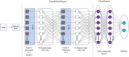
The architecture of a convolutional neural network is very similar to that of a conventional artificial neural network, especially in the final layer of the network, namely the fully connected layer. Additionally, it is noted that convolutional neural networks can accept multiple feature maps as input, rather than vectors (Figure 1).

Figure 1. General structure of a convolutional neural network.

2.1. DenseNet framework

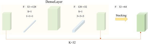
The skip connection, first proposed by the Residual Network (ResNet) (He et al. 2015), is a landmark innovation in the field of deep learning for computer vision. However, while ResNet ensures effective gradient updates during backpropagation, the use of skip connections for summation in forward propagation can lead to information bottlenecks. The Densely Connected Convolutional Network (DenseNet) (Huang et al. 2016) adopts the skip connection idea from ResNet but converts skip connections for summation into feature map concatenation during forward propagation. The main body of the network is composed of multiple DenseBlocks, with TransitionLayers added between DenseBlocks to reduce feature map resolution. A DenseBlock consists of several DenseLayers, with the stacking of feature maps occurring within the DenseLayer, as shown in Figure 2. In the figure, the green cubes represent feature maps, and the blue cubes represent convolution kernels. K represents the growth of feature maps in the DenseLayer, F represents the feature map channels, and S represents the convolution kernel stride. The original feature map first undergoes 1 × 1 × 1 convolution to adjust the number of channels for subsequent computations. Then, 3 × 3 × 3 convolution is applied to extract features. Subsequently, the computed feature map is stacked with the original feature map in the channel dimension to achieve multi-level feature reuse, significantly reducing the number of network parameters and enabling a deeper stack of network layers.

Figure 2. Schematic diagram of the DenseLayer.

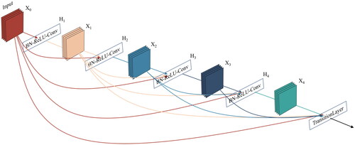
From the architecture connectivity depicted in Figure 3, it can be inferred that DenseNet does not draw representative strength from extremely deep or wide architectures but rather leverages functional reuse to explore the network’s potential, yielding streamlined models that are easy to train and have high parameter efficiency. The concatenation of feature maps learned by different layers introduces variations in the inputs of subsequent layers and improves efficiency. Compared to the capability of the Inception network to connect features from different layers, DenseNet is simpler and more efficient.

Figure 3. DenseNet architecture connectivity.

2.2. Group convolution (GC)

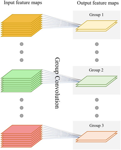
The emergence of AlexNet (Krizhevsky et al. 2012) demonstrated that, with the feature maps grouped, each group of feature maps can learn different dimensions of acoustic emission features. Building on this idea, the Aggregated Residual Transformations Neural Network (ResNeXt) (Xie et al. 2016) introduced Group Convolution (GC). In this study, GC is embedded in the 3 × 3 × 3 convolution of the DenseLayer, transforming the originally dense connections between the convolution kernels and channels into sparse connections, further reducing model parameters, as shown in Figure 4. Constructing group convolutions can lead to poor information flow between groups, hence, a 1 × 1 × 1 convolution layer is added after the group convolution in the DenseLayer to facilitate inter-group information fusion.

Figure 4. Schematic diagram of group convolution.

2.3. Squeeze-and-excitation (SE) module

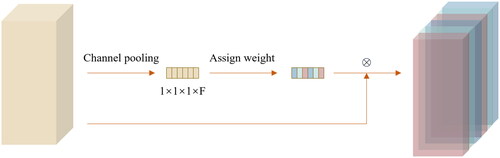
The Squeeze and Excitation Network (SeNet) (Hu et al. 2017) was the first to apply attention mechanisms in the field of computer vision, enabling the model to dynamically focus on important acoustic emission features. The "Squeeze-and-Excitation" (SE) module in the attention mechanism, as illustrated in Figure 5, shows equal channel weights in the left cube and unequal channel weights in the right cube. For each DenseLayer in the DenseBlock, after the final feature map computation, an additional branch is introduced to perform average pooling operation in the channel dimension (Squeeze). Subsequently, two fully connected layers compute the channel weights (Excitation), which are then multiplied channel-wise with the corresponding feature map (denoted as ⊗) to obtain the final output. The SE module can be easily embedded into any model structure, enabling the model to focus more on the acoustic emission features crucial for predicting coal and rock damage. This module effectively enhances model generalization while introducing only a small number of parameters.

Figure 5. Squeeze and excitation module illustration.

3. Construction of DenseNet + GC + SE model

3.1. Network architecture

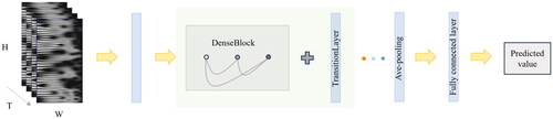
The network consists of three main parts: an initial 3D convolution to rapidly reduce feature map resolution, the cross-stacked DenseBlock and TransitionLayer (Trans_Layer) for feature extraction, and average pooling output. In Table 1, H, W, and T represent the height, width, and the number of consecutive stacked two-dimensional images in the feature map, while S denotes the convolutional kernel stride. The terms conv, FC, and pool respectively refer to the convolutional layer, fully connected layer, and pooling layer.

Table 1. DenseNet + GC + SE network architecture.

Network layer	Output dimension (T, W, H)	DenseNet + GC + SE
Convolution	16, 224, 112	7 × 7 × 7 conv S = (1, 2,2)
Max-Pool	8, 112, 56	3 × 3 × 3 pool, S = 2
Dense Block (1)	8, 112, 56	$\left[\begin{array}{c}{1}^{3}c\mathit{\text{onv}}\\ 3^{3}c\mathit{\text{onv}} g=16\\ 1^{3}c\mathit{\text{onv}}\end{array}\right]\times 3$
Trans_Layer (1)	8, 112, 56 4, 56, 28	1 × 1 × 1 conv_$g,$ S = 1 2 × 2 × 2 avg_pool
Dense Block (2)	4, 56, 28	$\left[\begin{array}{c}{1}^{3}c\mathit{\text{onv}}\\ 3^{3}c\mathit{\text{onv}} g=16\\ 1^{3}c\mathit{\text{onv}}\end{array}\right]\times 6$
Trans_Layer (2)	4, 56, 28 2, 28, 14	1 × 1 × 1 conv_$g,$ S = 1 2 × 2 × 2 avg_pool
Dense Block (3)	2, 28, 14	$\left[\begin{array}{c}{1}^{3}c\mathit{\text{onv}}\\ 3^{3}c\mathit{\text{onv}} \\ 1^{3}c\mathit{\text{onv}}\end{array}g=16\right]\times 12$
Trans_Layer (3)	2, 28, 14 1, 14, 7	1 × 1 × 1 conv_$g,$ S = 1 2 × 2 × 2 avg_pool
Dense Block (4)	1, 14, 7	$\left[\begin{array}{c}{1}^{3}c\mathit{\text{onv}}\\ 3^{3}c\mathit{\text{onv}}\\ 1^{3}c\mathit{\text{onv}}\end{array} g=16\right]\times 8$
Avg_Pool	–	Adapted avg_pool
FC	4	fully-connected

DenseNet effectively leverages multi-level features, allowing the model’s output to depend not only on the high-level features of subsequent convolutional layers but also on the low-level features of earlier convolutional layers, thereby reducing the number of feature map channels and significantly decreasing the network’s parameter count compared to the original C3D network. The number of groups in group convolution can serve as a measure of model complexity, and in the acoustic emission damage prediction model, it also serves to integrate multiple parameters of acoustic emission. When using acoustic emission precursor information to predict the instability and failure of coal and rock, parameters such as energy, amplitude, event counts, and fractals can be semantically related to the number of groups in group convolution, enabling the coupling analysis of multiple parameters of acoustic emission. Setting a larger number of groups in group convolution may allow the neural network to explore new acoustic emission features, which is beneficial for the generalization and unification of the acoustic emission recognition model.

The SE module can effectively improve the generalization ability of the acoustic emission damage prediction model and accelerate model training while adding a small number of model parameters. The network process is detailed in Figure 6, where the circles within the DenseBlock represent DenseLayers.

Figure 6. Illustrates the DenseNet network architecture and the data transmission process.

3.2. Model training

3.2.1. Forward propagation

Taking the jth DenseLayer in the ith DenseBlock as an example, let the input feature map be denoted as: $x_j^i,$ where $x_j^i\in R^{F\times T\times H\times W},$ with F representing the number of feature map channels; T denoting the number of feature map stacks in the temporal dimension; H and W representing the feature map resolution. Let $y_j^i$ be the output feature map. Define h($x_j^i$) as shown in Equation (1)(1) $$h(x_j^i)=1^3\_\mathit{\text{conv}}\{3^3\_\mathit{\text{conv}}\_g[1^3\_\mathit{\text{conv}}(x_j^i)\left]\right\}$$(1) : (1) $$h(x_j^i)=1^3\_\mathit{\text{conv}}\{3^3\_\mathit{\text{conv}}\_g[1^3\_\mathit{\text{conv}}(x_j^i)\left]\right\}$$(1)

The mapping from input to output, f, is defined as shown in Equation (2)(2) $$f:y_j^i=\mathit{\text{concat}}\{[h(x_j^i)],x_j^i\}$$(2) : (2) $$f:y_j^i=\mathit{\text{concat}}\{[h(x_j^i)],x_j^i\}$$(2)

In Equation (1)(1) $$h(x_j^i)=1^3\_\mathit{\text{conv}}\{3^3\_\mathit{\text{conv}}\_g[1^3\_\mathit{\text{conv}}(x_j^i)\left]\right\}$$(1) , conv represents the combination operation of convolution, batch normalization, and activation, as shown in Equation (3)(3) $$\mathit{\text{conv}}(x)=\mathit{\text{ReLU}}[\mathit{\text{batch}}\_\mathit{\text{norm}}(x*{\varphi }_j^{i,k})]$$(3) : (3) $$\mathit{\text{conv}}(x)=\mathit{\text{ReLU}}[\mathit{\text{batch}}\_\mathit{\text{norm}}(x*{\varphi }_j^{i,k})]$$(3)

The convolution calculation (symbol: *) is denoted. ${\varphi }_j^i$ represents the convolutional kernel parameters of the k-th feature map in the j-th layer of the DenseLayer, which are the primary parameters learned by the neural network, where k∈[1, 2, 3]. batch_norm represents the batch normalization operation, and ReLU represents the activation function, expressed as (4): (4) $$\mathit{\text{ReLU}}(x)=\mathrm{\text{max}}(0,x)$$(4)

Multiple DenseLayers form a DenseBlock, and TransitionLayer is added between DenseBlocks to achieve downsampling. TransitionLayer takes the output feature map of the previous DenseBlock as input, while using the pooling function to reduce the feature map resolution. After multiple DenseBlocks, TransitionLayers, and Pool modules are stacked, the model adds a fully connected layer (FC) to output the results and accomplish the classification of training samples.

3.2.2. Backpropagation

The definition of the training set cross-entropy loss is given by Equation (5)(5) $${\Upsilon }_{\mathit{\text{train}}}=-\frac{1}{B}\sum _l^{l+B}{y}_l\mathit{\text{lg}}{\widehat{y}}_l+(1-y_l)\mathit{\text{lg}}(1-y_l)$$(5) : (5) $${\Upsilon }_{\mathit{\text{train}}}=-\frac{1}{B}\sum _l^{l+B}{y}_l\mathit{\text{lg}}{\widehat{y}}_l+(1-y_l)\mathit{\text{lg}}(1-y_l)$$(5)

In the equation: ${\mathrm{\Upsilon }}_{\mathit{\text{train}}}$ denotes the training loss; l represents the l-th training sample; since it’s not possible to input all the data into the model at once during training, it needs to be fed in batches, where B is the batch size; $y_l$ is the true label of the training sample; and ${\widehat{y}}_l$ is the predicted label of the training sample. Minimizing the loss guides the optimization of the model. The Stochastic Gradient Descent (SGD) algorithm chooses the direction of the negative gradient to optimize the loss and update the model parameters, as shown in Equation (6)(6) $${\varphi }_j^{i,k}={\varphi }_j^{i,k}-\eta \frac{\partial {\Upsilon }_{\mathit{\text{train}}}}{\partial {\varphi }_j^{i,k}}$$(6) : (6) $${\varphi }_j^{i,k}={\varphi }_j^{i,k}-\eta \frac{\partial {\Upsilon }_{\mathit{\text{train}}}}{\partial {\varphi }_j^{i,k}}$$(6)

In the equation, $\eta$ represents the learning rate of the model. When all the batches have completed one round of iteration, it is referred to as completing one Epoch of the data.

3.2.3. Experimental procedure

1. Input the training dataset $\Omega :[x_l；y_l],$ where $x_l\in R^{F\times T\times H\times W}$ and $y_l\in N_{+},$ and the training parameters K, B, and $\eta .$

2. Sample B data points from the training set and perform forward propagation according to the network structure shown in Table 1 to achieve training sample classification.

3. Calculate the cross-entropy loss between the forward propagated sample predicted label ${\widehat{y}}_l$ and the sample true label $y_l.$

4. Use the SGD algorithm to update the model parameters.

5. Repeat steps (1), (2), (3), and (4) until the model converges.

3.3. Model evaluation metrics

To validate and evaluate the effectiveness of the proposed method in this study, the selected evaluation metrics include accuracy, precision, recall, and F1 score, which measure the performance of different models. The models were trained for 30 epochs, and the dataset in the experiment was uniformly distributed.

For the multi-classification task in this experiment, the true class of the samples is identified as the positive class, while all other classes are identified as the negative class. Firstly, TP is defined as the true positive samples predicted as positive by the model; TN is the true negative samples predicted as negative by the model; FP is the false positive samples predicted as positive by the model; FN is the false negative samples predicted as negative by the model.

1. Model Complexity: Model complexity reflects the number of parameters contained in the model (unit: MB). The more parameters there are, the more complex the model is.

2. Time Complexity: Time complexity represents the time consumed for a validation sample to go from input to output in the model (unit: ms). The longer the time it takes, the lower the efficiency of the model.

3. Accuracy: The percentage of samples correctly predicted by the classification model out of the total samples, with a higher value indicating better predictive performance of the model. (7) $$\mathit{\text{Accuracy}}=\frac{(\mathit{\text{TP}}+\mathit{\text{TN}})}{(\mathit{\text{TP}}+\mathit{\text{TN}}+\mathit{\text{FP}}+\mathit{\text{FN}})}$$(7)

4. Precision: The proportion of the number of samples predicted as positive by the classification model to the total number of samples predicted as positive, with a higher value indicating more accurate positive predictions by the model. (8) $$\mathit{\text{Precision}}=\frac{\mathit{\text{TP}}}{(\mathit{\text{TP}}+\mathit{\text{FP}})}$$(8)

5. Recall is the proportion of the number of truly positive samples in the samples predicted as positive by the classification model to the total number of positive samples, with a higher value indicating that the model predicts more comprehensive positive samples. (9) $$\mathit{\text{Recall}}=\frac{\mathit{\text{TP}}}{(\mathit{\text{TP}}+\mathit{\text{FN}})}$$(9)

6. The F1 score is a metric that evaluates the model by considering both precision and recall, which helps balance the relationship between the two. A higher value indicates better model performance. (10) $${\mathit{F}}_{\mathit{1}}=\frac{\mathit{2}*\mathit{\text{Precision}}*\mathit{\text{Recall}}}{(\mathit{\text{Precision}}+\mathit{\text{Recall}})}$$(10)

4. Acoustic emission experiment and data processing

4.1. Acquiring precursor information in acoustic emission experiments

The evolution of acoustic emission in coal and rock can reflect the intrinsic damage processes. Based on this, laboratory research was conducted to predict coal and rock damage using acoustic emission signals. The experimental samples were taken from the 3rd coal seam in the 7th mining area of Xinglongzhuang Coal Mine in Yanzhou District, Jining, Shandong. These samples were processed into standard cylindrical specimens (φ 50 mm × L100 mm). Each specimen was equipped with 6 miniature sensors to receive acoustic emission signals. The experiments were conducted using the AE-DS5-8A Full Information Acoustic Emission Signal Analyzer, as illustrated in Figure 7.

Figure 7. Schematic layout of the experimental setup with acoustic emission sensors.

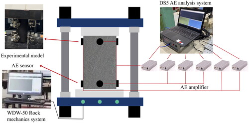
During the experiment, in conjunction with the acoustic emission acquisition system, real-time collection of the sample’s acoustic emission damage events, positioning, amplitude parameters, and the entire waveform under uniaxial compression displacement loading were captured until the sample experienced unstable fracture. The waveform of the acoustic emission event is determined automatically by the acquisition system by combining the time difference of the first impact arrival of the event to different sensors and the coal sample wave velocity measured from the lead-breakage test. The physical and mechanical parameters of the sample and its loading rate are detailed in Table 2. As the acoustic emission amplitude propagates within the coal sample, it gradually attenuates with increasing distance. Therefore, based on the pre-test lead-breakage test, the amplitude attenuation curve with distance is constructed to compensate for the attenuation of the source amplitude. Even if a small amount of acoustic emission signals are missed, the neural network can still accurately fit the basic distribution characteristics of parameters such as acoustic emission events, positioning, and amplitude during the training process (Liu et al. 2020b).

Table 2. Physical and mechanical parameters of the sample and loading rate.

Sample number	Radius /mm	Height /mm	Density /(kg·m^-3)	Failure stress /MPa	Loading rate /(mm·min^–1)
N1	24.80	100.10	1.25	12.34	0.2
N2	24.85	100.32	1.23	12.56	0.2
N3	24.79	100.24	1.24	12.98	0.2
N4	24.84	100.25	1.23	13.87	0.2

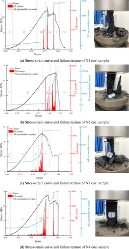
As shown in Figure 8, the stress-strain curves exhibit a common trend, but there are significant differences in detail. The similarity of this trend is related to the common characteristics of the coal seam, but the differences in the physical properties and structural variations of different coal samples lead to distinct manifestations in the specific details of the curve (Liu et al. 2023). The gray dashed lines in the figure delineate Stages I to VI, representing distinct phases of coal sample failure. In the stress-strain curve shown in Figure 8, the damage classification principle divides the specimen’s behavior into several stages. The initial compaction stage represents the influence of external forces on the specimen, exhibiting linear elastic behavior where stress and strain are proportional. The compaction stage occurs when the specimen exceeds the linear elastic range but has not reached the yield point, causing the stress-strain curve to show nonlinear changes.The plastic deformation stage begins when observable plastic deformation appears, and the stress-strain curve exhibits a distinct yield point. The peak stress stage occurs after the yield point, where the specimen continues to undergo plastic deformation, but its hardness gradually increases, resulting in an upward trend in the curve.The onset of fracture stage is characterized by the specimen showing local necking, with stress concentrating in a specific area, leading to a sharp decline in the curve. The post-peak failure stage is when the specimen completely fractures, and the stress-strain curve rapidly drops to zero. Furthermore, under the same experimental conditions, the destruction process of different coal samples in the same coal seam also presents diversity (Hou et al. 2023). Through the recognition of experimental data images of multiple samples at different stages of destruction using the three-dimensional convolutional neural network, the model’s generalization ability is improved to enable more accurate differentiation of different samples. Training and application of the three-dimensional convolutional model can better identify and predict the behavior of coal seam damage, providing strong support for research and applications in related fields.

Figure 8. Uniaxial compression experimental results.

4.2. Data preprocessing

4.2.1. Experimental data

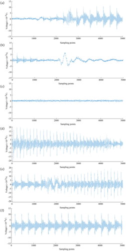
Using the AE_DS5 software, the loading process of the coal sample was replayed, and the average values of the acoustic emission damage events, locations, and amplitudes for each sensor during the uniaxial compression process were stored. The entire experimental process was divided into six stages according to the process of rock failure: initial compaction stage, compaction stage, plastic deformation stage, peak stress stage, fracture initiation stage, and post-peak failure stage. As shown in Figure 9, different waveform images appear during the six stages of coal and rock failure.

Figure 9. Acoustic emission waveforms at different stages. (a) Stage one (b) stage two (c) stage three (d) stage four (e) stage five (f) stage six.

4.2.2. Continuous wavelet transform (CWT)

The data processing was performed using the full process acoustic emission waveforms directly generated by the AE-DS5-8A full-information acoustic emission signal analyzer. After analyzing the common waveform, short-time Fourier transform, and continuous wavelet transform (CWT), it was found that CWT analysis is more conducive to feature extraction for the neural network constructed in this paper. In comparison to the short-time Fourier transform, wavelet transform is characterized by its window adaptability, with high frequency signal resolution and high low-frequency signal frequency resolution. In the context of engineering experiments, the focus is on the time at which low-frequency frequencies and high frequencies occur during the loading process, making the wavelet transform a theoretically sound choice for analyzing rock failure waveforms (Cheng et al. 2021). The core of this study is to predict and identify the specific stage of failure at a certain moment during the loading process of the coal sample and the time determined for this stage, with the identification accuracy supporting up to seconds. Therefore, this experiment was based on the real-time acquisition of acoustic emission parameters during the coal sample’s damage and failure process, including waveform data of acoustic emission events, the amplitude of events, and the time of occurrence, all collected data were in second-level continuous data that could be directly processed.

Using the AE-DS5 acoustic emission collection software, the loading process of the coal sample was replayed, and the average values of the acoustic emission damage events, location, and amplitude for each sensor during the uniaxial compression process were stored to construct the acoustic emission waveform-time evolution diagram. To meet the neural network’s requirement for learning a large number of data points, the number of decomposed waveform points in the MATLAB program was increased to 5000, aiming to display the waveform’s characteristics over a longer period and enhance the model’s generalization ability. Different segments of the waveform analysis were used to explain the varying characteristics of the acoustic emission during the rock failure process. The wavelet property of the Morlet wavelet can be expressed using complex trigonometric functions for wave oscillation or decay functions for smaller waves. Mathematically, this type of wavelet is called finite support. The finite support of the Morlet wavelet is achieved through an exponential decay function. The combination of complex trigonometric functions enables it to analyze frequency, while the decay function allows it to localize time, making the Morlet wavelet suitable for time-frequency analysis. Unless otherwise specified, the term CWT in this paper refers to the Morlet continuous wavelet transform, with the expression of the Morlet wavelet base function following the formula below: (11) $$\psi (t)=\mathrm{\text{exp}}({\mathrm{i}\mathrm{\omega }}_{{}_0}\mathrm{t})\mathrm{\text{exp}}(-\frac{{\mathrm{t}}^2}{2})$$(11)

The base function of the Morlet wavelet is composed of a complex trigonometric function multiplied by an exponential decay function. Here, ${\omega }_0$ represents the central frequency. The scale is commonly used to measure the frequency f of the wavelet, and the relationship between the two is given by: (12) $$\mathit{\text{Scale}}*f=\mathit{\text{Fs}}*{\omega }_0$$(12)

In the formula, Fs represents the sampling frequency of the signal, and ${\omega }_0$ is the Wave Central Freq. (13) $$\begin{array}{c}\underset{¯}{\overline{\psi }}f(a,b)={\int }_{-\infty }^{+\infty }\mathrm{f}(t){\overline{\psi }}_{a,b}(t)\mathit{\text{dt}}\\ ={\int }_{-\infty }^{+\infty }\mathrm{f}(t)\hspace{0.17em}\mathrm{\text{exp}}\hspace{0.17em}(-i{\omega }_0\frac{(t-b)}{a})\mathrm{\text{exp}}(-\frac{{(t-b)}^2}{2a^2})\mathit{\text{dt}}\end{array}$$(13)

The above formula is used to derive the formula for the Morlet wavelet transform by determining the wavelet base function and scale conversion. The CWT method selects a central frequency, then obtains many central frequencies through scale transformation, and generates a series of different interval base functions through time shifting. These functions are multiplied with the corresponding base function intervals of the original signal, and the resulting extremum corresponds to the frequency contained in that interval of the original signal.

As shown in Figure 10, each plot after data processing is divided into two parts. The top and bottom plots illustrate the number of frequencies present in the wavelet decomposition of the acoustic emission waveform at different scales. These plots can be used to display the amplitude changes of the waveform data in different time domains and scales, aiding in the analysis of time and frequency information of the waveforms. A darker color indicates a greater presence of data at the same time, which can be used to analyze the differences in the acoustic emission waveform at different stages of damage.

Figure 10. Waveform after wavelet transform of acoustic emission. (a) Stage one (b) stage two (c) stage three (d) stage four (e) stage five (f) stage six.

4.2.3. YOLOv5s network structure Image processing

After the wavelet analysis processing, the images have a relatively high resolution, resulting in excessive time consumption during network analysis. Therefore, based on the wavelet analysis, the training and validation sets for acoustic emission signal recognition continue to undergo YOLO grid processing to achieve rapid model recognition while preserving the image features without loss (Cong et al. 2023). The YOLOv5 official code provides four versions of the object detection network, namely Yolov5s, Yolov5m, Yolov5l, and Yolov5x. As shown in Table 3, these models have the same basic structure, with differences in model depth and width as parameters. YOLOv5s is the shallowest network in the YOLOv5 series, with the smallest feature map width. The other three models progressively deepen and widen based on this.

Table 3. YOLO model performance comparison table.

Model	Size (pixels)	mAP^val 0.5:0.95	mAP^val 0.5	Speed V100 b1 (ms)	Speed V100 b1 (ms)	Speed V100 b32 (ms)	Params (M)	FLOPs @640(B)
YOLOv5n	640	28.0	45.7	45	6.3	0.6	1.9	4.5
YOLOv5s	640	37.4	56.8	98	6.4	0.9	7.2	16.5
YOLOv5m	640	45.4	64.1	224	8.2	1.7	21.2	49.0
YOLOv5l	640	49.0	67.3	430	10.1	2.7	46.5	109.1
YOLOv5x	640	50.7	68.9	766	12.1	4.8	86.7	205.7

Figure 11 compares the performance of different YOLOv5 grids in the COCO training set, and YOLOv5s is chosen to achieve a balance between speed and accuracy. Its smaller model size is suitable for real-time applications and is easy to train and deploy. Figure 12 shows the network structure of Yolov5s, which consists of four parts: Input End, Backbone, Neck, and Prediction.

Figure 11. YOLOv5 algorithm performance test for each version.

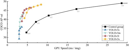
Figure 12. YOLOv5s structure diagram.

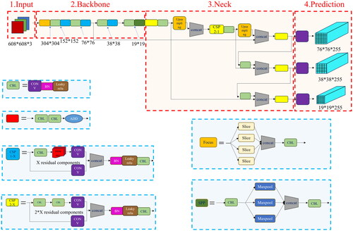
Through the Mosaic data augmentation and adaptive anchor box calculation at the input end; the Focus and CSP structures in the backbone network; the FPN + PAN structure in the neck network; and the GIOU_Loss architecture in Prediction, YOLO grid processing achieves the following four objectives, which are also the advantages of YOLO grid processing: enriching the dataset, enhancing model robustness, strengthening batch normalization, and improving small object detection performance.

In deep learning, fully connected layers are typically used to transform the dimensions of features from convolutional layers to the output layer. However, when dealing with high-dimensional and nonlinear features, fully connected layers involve significant computational overhead and can lead to issues such as overfitting. Image processing through the YOLO architecture can effectively avoid overfitting issues caused by excessive repetition of image features, accelerate the model’s training and inference process, and further enhance the model’s performance.

5. Results of acoustic emission recognition model

5.1. Selection of training parameters

A six-classification model based on the method of acoustic emission waveform spectrogram classification was constructed to identify the stages of coal sample damage using a neural network approach. The DenseNet network was used for recognition, and the experiments were conducted using a single GTX 3070 GPU for training. The model parameters used for training are detailed in Table 4.

Table 4. Model training parameters.

Input (F, T, H, W)	Lr	Epochs	Training samples	Loss	Optimization method	DeneLayer	GC Parameters
1, 16, 256, 256	0.1	30	4088	XApEn	SGD	32	16

5.2. Experimental model result analysis

5.2.1. Comparative analysis of training results

The model performance and evaluation metrics are detailed in Table 5. According to the table, the four network structures (DenseNet, DenseNet + GC, DenseNet + SE, and DenseNet + GC + SE) achieved an accuracy higher than 98.29% on the validation set, with the highest being 99.51%. The sample recall rates were all above 98.02%, indicating that the 3D convolutional network can effectively fit spatiotemporal features. Compared to DenseNet + SE, DenseNet + GC + SE saw a 53.7% reduction in parameter count and a 36.4% reduction in time complexity, while the accuracy only decreased by 0.12%. This suggests that group convolution can effectively reduce the model load while ensuring model accuracy, making it easier to deploy the model in mining operations. Compared to DenseNet + GC, DenseNet + GC + SE saw a 71.4% reduction in time complexity, with only a 0.1% increase in parameter count. Although the integration of the attention mechanism slightly increased the parameter count, it significantly reduced the model’s time complexity and improved its efficiency.

Table 5. Validation set training results.

Network structure	Parameter/MB	Time complexity/ms	Accuracy/%	Recall/%	F1 score/%
DenseNet	30.01	1350 ± 66.1	98.90	98.02	98.46
DenseNet + GC	13.81	686 ± 23.7	98.29	98.02	98.15
DenseNet + SE	30.07	308 ± 15.4	99.51	99.50	99.50
DenseNet + GC + SE	13.92	196 ± 11.1	99.39	99.20	99.29

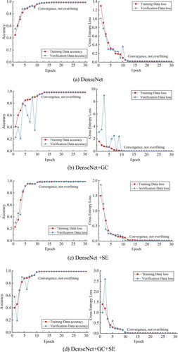
Figure 13 illustrates the changes in accuracy and cross-entropy loss during the training process of the DenseNet network structure. As shown in the graph, the DenseNet network structure eventually converges without overfitting (Huang et al. 2019), indicating that the model can effectively recognize the stages of damage in the validation set and learn the specific evolution patterns of acoustic emission within coal and rock samples.

Figure 13. Training/validation set – accuracy and cross-entropy loss.

Based on the DenseNet + GC + SE network, the predicted probability distributions for all validation samples were calculated, and the mean values were computed for different risk levels. See the confusion matrix in Figure 14 for the identification results (Rakkiyappan et al. 2015). The stages 1 to 6 correspond to the initial compaction stage, compaction stage, plastic deformation stage, peak stress stage, onset of fracture stage, and post-peak failure stage, respectively.

Figure 14. Probability distribution of output for validation samples.

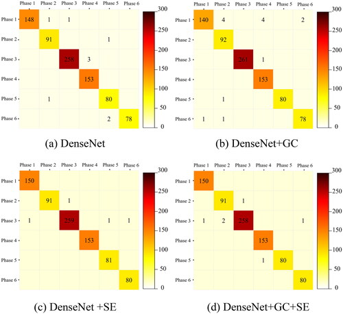
The confusion matrix’s columns represent the predicted categories, while the rows represent the true categories. The values in the confusion matrix are incremented by 1 at the corresponding position of the true row and predicted column for each sample in the validation set. Therefore, in Figure 13, the larger the values on the diagonal axis and the darker the color of the confusion matrix grid, the denser the samples are. From the figure, it can be observed that the predicted sample distribution is clustered near the main diagonal of the confusion matrix. Compared with the true sample categories, the fluctuation range is small, and the output probabilities tend to be concentrated, indicating that the model can effectively distinguish different stages of coal-rock damage. This further demonstrates that the model has effectively learned the specific evolution patterns of the internal acoustic emission in coal and rock.

5.2.2. The roles of GC and SE in acoustic emission feature extraction

For a qualitative analysis of the specific role of group convolution in the acoustic emission recognition model, enhancing the interpretability of the model, based on the DenseNet + GC + SE network, the output feature maps after grouping in the last layer of the third and fourth DenseBlocks of the model were calculated. The average of all pixels in each group of feature maps was computed to study the diversity of acoustic emission features. See Figure 15 for details.

Figure 15. The utility of group convolution in characterizing the diversity of acoustic emission features.

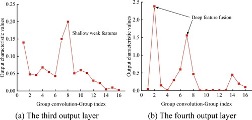
The values on the x-axis of Figure 15 represent the indices of each group in the group convolution, which can correspond to single or coupled acoustic emission features in some semantic sense. The y-axis represents the mean of all pixels in each group’s feature map. According to Figure 15, in the third DenseBlock, the output feature values are relatively small, distributed in the range of 0 to 0.25. This suggests that the model learns single and less correlated shallow information such as acoustic emission amplitude and fractals. In the fourth DenseBlock, the output feature values are highly concentrated, distributed in the range of 0 to 2.50, indicating that the model learns coupled features crucial for predicting coal and rock damage, such as event counts, fractals, and amplitude, forming a peak of feature fusion.For a qualitative analysis of the specific role of the SE module in the acoustic emission damage prediction model, based on the DenseNet + GC + SE network, the weights distribution along the channel dimension of the SE branch of the last DenseLayer in the second and fourth DenseBlocks of the model is obtained to study the importance of acoustic emission features, as shown in Figure 16.

Figure 16. The utility of the SE module – representing the importance of acoustic emission features.

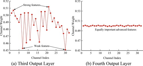
The abscissa of Figure 16 represents the channel index after the weight distribution in the SE module, where each channel corresponds to a certain acoustic emission single or coupled feature in a certain semantic sense. The ordinate represents the weight values of each channel. From Figure 16, it can be observed that there is a large variance in the weight values between different channels in the second DenseBlock, indicating that the model embedded with the SE module can pay more attention to important features favorable for coal-rock damage prediction. For instance, the model considers the acoustic emission amplitude feature as a key feature influencing the final coal-rock damage identification, thereby increasing the weight values of the amplitude feature. In the fourth DenseBlock, the weight values of each channel are almost equal, forming an approximately straight line, indicating that the model has learned equally important acoustic emission coupled features in the later stages.

6. Discussion

In this study, a three-dimensional convolutional neural network was employed to predict coal-rock damage, yielding favorable predictive results. While traditional 3D convolution effectively integrates spatiotemporal features, it suffers from excessive parameters and inefficiency. Therefore, a lightweight convolutional neural network model, DenseNet + GC + SE, was introduced.

Under the same conditions, considering one convolutional layer of the traditional C3D network and DenseNet + GC, let the input feature map channel be F1, the output feature map dimensions be height H, width W, and channel F2, and the feature map temporal dimension stacking be T, and the convolutional kernel size be D. The computational costs and parameters are as follows: D3·H·W·F1·F2·T and D3·F1·F2·T.

Based on one layer of DenseLayer, let Growth_Rate be denoted as K, the input feature map channel as g, and the input and output feature maps consistent with C3D. The computational cost and parameter count for this layer can be computed as follows: T·H·W·4K(F1 + D3·4K/g + K) and T·4K(F1+ D3·4K/g + K), respectively. The ratio of computational cost and parameter count is (D3·F1·F2)/(4K(F1+ D3·4K/g + K)).

Due to the fact that K≪F1 or F2 in the deep layers of the neural network, embedding group convolution in DenseNet can significantly reduce both the computational cost and the parameter count, enabling deeper network stacking.

The core idea of the SE module is to enable the network to learn feature weights based on the loss, such that effective feature maps have larger weights and ineffective or less effective feature maps have smaller weights. This training strategy helps the model achieve better results and is easily deployable, without the need to introduce new functions or layers. In addition, it has favorable characteristics in terms of model and computational complexity. Specific parameter variations are detailed in Table 6.

Table 6. Comparison of different 3D network performances.

Network structure	Parameter /MB	Depth	Time complexity/ms
C3D	>120	11	/
DenseNet + GC	13.81	92	686 ± 23.7
DenseNet + GC + SE	13.92	92	196 ± 11.1

The acoustic emission test in this study was only conducted on coal samples from the No. 3 coal seam in the Xinglongzhuang mining area of Yanzhou, Jining, Shandong. The samples were subjected to uniaxial compression displacement loading under quasi-static conditions. Subsequent research could be extended to different types of coal samples by applying methods such as confining pressure and dynamic loading to enhance the acoustic emission-based deep learning prediction method for coal-rock failure (Liu et al. 2018; Xu et al. 2021). Various methods are available for predicting coal-rock instability, and acoustic emission is just one of them. In the future, a multi-method and multi-parameter collaborative prediction system can be established by synthesizing deformation or fissure fields during coal-rock instability, complementing the acoustic emission technique.

To facilitate the practical deployment of the model, even on mobile mining equipment or embedded devices, further network lightweighting can be considered, simplifying group convolutions to depth convolutions (Shrestha and Mahmood 2019). Other model compression methods, such as channel rearrangement (Zhang et al. 2017) and knowledge distillation (Radosavovic et al. 2017), can be introduced to strike a balance between efficiency and accuracy.

In China, the microseismic method is widely used to monitor and warn of dynamic disasters in coal mines (Liu et al. 2021b; Yuan et al. 2023). Acoustic emission shares the same principle as microseismicity, differing only in the lower magnitude and higher frequency of acoustic emission. Therefore, lightweight 3D convolution, as a new means of coal-rock failure prediction, can be extended to specified mines. Based on the microseismic signals in the mine, a lightweight 3D convolution microseismic failure prediction model can be constructed (Cui et al. 2021), aiming to predict underground dynamic disasters. Real-time collection of microseismic signals in hazardous areas underground can be preprocessed into two-dimensional image sequences containing microseismic events, magnitude, and location as inputs for the model, enabling the real-time identification of the moment of coal-rock dynamic disaster occurrence and providing new insights for research on dynamic instability disaster early warning in coal mines.

7. Conclusion

This study has constructed a lightweight 3D convolution prediction model based on the acoustic emission characteristics before coal-rock failure, integrating multidimensional spatial-temporal information to identify coal-rock failure. The main conclusions are as follows:

1. The 3D convolution model can effectively predict the identification of the coal sample’s failure stage based on the acoustic emission signal. The four network structures (DenseNet, DenseNet + GC, DenseNet + SE, and DenseNet + GC + SE) did not experience overfitting, with accuracy on the validation set exceeding 98.29%, reaching a maximum of 99.51%, and sample recall rates exceeding 98.02%. The output probability of the DenseNet + GC + SE model tends to be a single-point distribution, indicating its ability to distinguish between different stages of failure. The embedding of group convolutions and SE modules can effectively improve model efficiency. Compared to the DenseNet + SE network, the DenseNet + GC + SE model reduces the parameter count by 53.7% and time complexity by 36.4%, while compared to the DenseNet + GC network, the time complexity is reduced by 71.4%. The DenseNet + GC + SE model exhibits the best performance, effectively learning the specific evolution of acoustic emissions inside coal-rock while ensuring model efficiency.

2. The integration of group convolutions into the DenseNet + GC + SE network can affect the coupling of multiple parameters in acoustic emissions, representing the diversity of acoustic emission characteristics. The integration of the SE module can evaluate the importance of acoustic emission features.

3. The lightweight 3D convolution model, DenseNet + GC + SE, can effectively identify coal-rock failure stages based on acoustic emission signals, with the predicted sample distribution near the main diagonal of the confusion matrix. The DenseNet + GC + SE model can be extended to predict the failure of different types of coal samples or applied to underground disaster prediction.

Author contributions

T.W. and L.L. wrote the main manuscript text, Z.L. conducted the experiments, T.W. modified the manuscript text, L.L. prepared figures. All authors reviewed the manuscript.

Disclosure statement

The authors declare that they have no known competing financial interests or personal relationships that could have appeared to influence the work reported in this paper.

Data availability statement

All the data, models or code generated or used in the present study are available from the corresponding author by request.

Correction Statement

This article has been corrected with minor changes. These changes do not impact the academic content of the article.

Additional information

Funding

This work was funded by National Science Foundation of China [Grant Nos. 52004015, 51874014, and 52311530070], the fellowship of China National Postdoctoral Program for Innovative Talents [Grant No. BX2021033], the fellowship of China Postdoctoral Science Foundation [Grant Nos. 2021M700389 and 2023T0025], and the Fundamental Research Funds for the Central Universities of China [Grant No. FRF-IDRY-20-003].

References

- Bai Q, Zhang C, Paul Young R. 2022. Using true-triaxial stress path to simulate excavation-induced rock damage: a case study. Int J Coal Sci Technol. 9(1):16. doi: 10.1007/s40789-022-00522-z.
- Cheng X. 2019. Damage and failure characteristics of rock similar materials with pre-existing cracks. Int J Coal Sci Technol. 6(4):505–517. doi: 10.1007/s40789-019-0263-4.
- Cheng Y, Lin M, Wu J, Zhu H, Shao X. 2021. Intelligent fault diagnosis of rotating machinery based on continuous wavelet transform-local binary convolutional neural network. Knowl. Based Syst. 216:106796. doi: 10.1016/j.knosys.2021.106796.
- Chi X, Yang K, Wei Z. 2021. Breaking and mining-induced stress evolution of overlying strata in the working face of a steeply dipping coal seam. Int J Coal Sci Technol. 8(4):614–625. doi: 10.1007/s40789-020-00392-3.
- Cong X, Li S, Chen F, Liu C, Meng Y. 2023. A review of YOLO object detection algorithms based on deep learning. Front Comput Intel Syst. 4(2):17–20. doi: 10.54097/fcis.v4i2.9730.
- Cui B, Dong X-m, Zhan Q, Peng J, Sun W. 2021. LiteDepthwiseNet: a lightweight network for hyperspectral image classification. IEEE Transactions on Geoscience and Remote Sensing p. 60:1-15. doi: 10.48550/arXiv.2010.07726.
- Di Y, Wang E, Li Z, Liu X, Li B. 2021. Method for EMR and AE interference signal identification in coal rock mining based on recurrent neural networks. Earth Sci Inform. 14(3):1521–1536. doi: 10.1007/s12145-021-00658-7.
- Dou L, Yang K, Chi X. 2020. Fracture behavior and acoustic emission characteristics of sandstone samples with inclined precracks. Int J Coal Sci Technol. 8(1):77–87. doi: 10.1007/s40789-020-00344-x.
- Guo P, Zhang P, Bu M, Xing H, He M. 2023. Impact of cooling rate on mechanical properties and failure mechanism of sandstone under thermal–mechanical coupling effect. Int J Coal Sci Technol. 10(1):7. doi: 10.1007/s40789-023-00584-7.
- He K, Zhang X, Ren S, Sun J. 2015. Deep residual learning for image recognition. 2016 IEEE conference on computer vision and pattern recognition (CVPR):770-778. doi: 10.1109/CVPR.2016.90.
- Hou W, Ma D, Li Q, Zhang J, Liu Y, Zhou C. 2023. Mechanical and hydraulic properties of fault rocks under multi-stage cyclic loading and unloading. Int J Coal Sci Technol. 10(1). doi: 10.1007/s40789-023-00618-0.
- Hu J, Shen L, Albanie S, Sun G, Wu E. 2017. Squeeze-and-excitation networks. 2018 IEEE/CVF conference on computer vision and pattern recognition:7132-7141. doi: 10.48550/arXiv.1709.01507.
- Huang G, Liu Z, Weinberger KQ. 2016. Densely Connected Convolutional Networks. 2017 IEEE Conference on Computer Vision and Pattern Recognition (CVPR):2261-2269. doi: 10.48550/arXiv.1608.06993.
- Huang J, Qu L, Jia R, Zhao B. 2019. O2U-Net: a simple noisy label detection approach for deep neural networks. 2019 IEEE/CVF international conference on computer vision (ICCV):3325–3333. doi: 10.1109/ICCV.2019.00342.
- Kong X, Wang E, Hu S, Shen R, Li X, Zhan T. 2016. Fractal characteristics and acoustic emission of coal containing methane in triaxial compression failure. J Appl Geophys. 124:139–147. doi: 10.1016/j.jappgeo.2015.11.018.
- Krizhevsky A, Sutskever I, Hinton GE. 2012. ImageNet classification with deep convolutional neural networks. Commun ACM. 60(6):84–90. doi: 10.1145/3065386.
- Li H, Li H. 2017. Mechanical properties and acoustic emission characteristics of thick hard roof sandstone in Shendong coal field. Int J Coal Sci Technol. 4(2):147–158. doi: 10.1007/s40789-017-0163-4.
- Liu B, Zhao Y, Zhang C, Zhou J, Li Y, Sun Z. 2021a. Characteristic strength and acoustic emission properties of weakly cemented sandstone at different depths under uniaxial compression. Int J Coal Sci Technol. 8(6):1288–1301. doi: 10.1007/s40789-021-00462-0.
- Liu H, Feng X, Liu L, Li T, Tang C. 2023. Mechanical properties and failure characteristics of anisotropic shale with circular hole under combined dynamic and static loading. Int J Rock Mech Min Sci. 170:105524. doi: 10.1016/j.ijrmms.2023.105524.
- Liu L, Ji H, Elsworth D, Zhi S, Lv X, Wang T. 2020a. Dual-damage constitutive model to define thermal damage in rock. Int J Rock Mech Min Sci. 126:104185. doi: 10.1016/j.ijrmms.2019.104185.
- Liu L, Zhu W, Wei C, Elsworth D, Wang J. 2018. Microcrack-based geomechanical modeling of rock-gas interaction during supercritical CO2 fracturing. J Petrol Sci Eng. 164:91–102. doi: 10.1016/j.petrol.2018.01.049.
- Liu L, Zhang Z, Wang T, Zhi S, Wang J. 2024. Evolution characteristics of fracture volume and acoustic emission entropy of monzogranite under cyclic loading. Geomech Geophys Geo-Energ Geo-Resour. 10(1):16. doi: 10.1007/s40948-024-00737-1.
- Liu L, Ji H, Lü X, Wang T, Zhi S, Pei F, Quan D. 2021b. Mitigation of greenhouse gases released from mining activities: a review. Int J Miner Metall Mater. 28(4):513–521. doi: 10.1007/s12613-020-2155-4.
- Liu X, Liu Z, Li X, Gong F, Du K. 2020b. Experimental study on the effect of strain rate on rock acoustic emission characteristics. Int J Rock Mech Min Sci. 133:104420. doi: 10.1016/j.ijrmms.2020.104420.
- Nikolenko PV, Epshtein SA, Shkuratnik VL, Anufrenkova PS. 2020. Experimental study of coal fracture dynamics under the influence of cyclic freezing–thawing using shear elastic waves. Int J Coal Sci Technol. 8(4):562–574. doi: 10.1007/s40789-020-00352-x.
- Qian Y, Li Q, Hu Q, Jiang Z, Liu R, Li J, Li W, Yu C. 2023. Extraction and identification of spectrum characteristics of coal and rock hydraulic fracturing and uniaxial compression signals. Int J Coal Sci Technol. 10(1):8. doi: 10.1007/s40789-023-00610-8.
- Qiu Z, Yao T, Mei T. 2017. Learning spatio-temporal representation with Pseudo-3D residual networks. 2017 IEEE International Conference on Computer Vision (ICCV):5534–5542. doi: 10.1109/ICCV.2017.590.
- Radosavovic I, Dollár P, Girshick RB, Gkioxari G, He K. 2017. Data distillation: towards omni-supervised learning. 2018 IEEE/CVF conference on computer vision and pattern recognition:4119-4128. doi: 10.48550/arXiv.1712.04440.
- Rakkiyappan R, Cao J, Velmurugan G. 2015. Existence and uniform stability analysis of fractional-order complex-valued neural networks with time delays. IEEE Trans Neural Netw Learn Syst. 26(1):84–97. doi: 10.1109/TNNLS.2014.2311099.
- Sainath TN, Vinyals O, Senior AW, Sak H. 2015. Convolutional, long short-term memory, fully connected deep neural networks. 2015 IEEE International Conference on Acoustics, Speech and Signal Processing (ICASSP):4580–4584. doi: 10.1109/ICASSP.2015.7178838.
- Shrestha AK, Mahmood A. 2019. Review of deep learning algorithms and architectures. IEEE Access. 7:53040–53065. doi: 10.1109/ACCESS.2019.2912200.
- Song S, Ren T-x, Dou L, Sun J, Yang X, Tan L. 2023a. Fracture features of brittle coal under uniaxial and cyclic compression loads. Int J Coal Sci Technol. 10(1). doi: 10.1007/s40789-023-00564-x.
- Song Z, Wu Y, Zhang Y, Yang Y, Yang Z. 2023b. Mechanical responses and acoustic emission behaviors of coal under compressive differential cyclic loading (DCL): a numerical study via 3D heterogeneous particle model. Int J Coal Sci Technol. 10(1):2. doi: 10.1007/s40789-023-00589-2.
- Tang J, Zhang X, Sun S-j, Pan Y, Li L. 2022. Evolution characteristics of precursor information of coal and gas outburst in deep rock cross-cut coal uncovering. Int J Coal Sci Technol. 9(1):13. doi: 10.1007/s40789-022-00471-7.
- Tran D, Bourdev LD, Fergus R, Torresani L, Paluri M. 2014. Learning spatiotemporal features with 3D convolutional networks. 2015 IEEE International Conference on Computer Vision (ICCV):4489–4497. doi: 10.1109/ICCV.2015.510.
- Xie S, Girshick RB, Dollár P, Tu Z, He K. 2016. Aggregated residual transformations for deep neural networks. 2017 IEEE Conference on Computer Vision and Pattern Recognition (CVPR):5987-5995. doi: 10.1109/CVPR.2017.634.
- Xu T, Fu M, Yang S-q, Heap MJ, Zhou G-l 2021. A numerical meso-scale elasto-plastic damage model for modeling the deformation and fracturing of sandstone under cyclic loading. Rock Mech Rock Eng. 54(9):4569–4591. doi: 10.1007/s00603-021-02556-2.
- Xue D, Lu L, Zhou J, Lu L, Liu Y. 2020. Cluster modeling of the short-range correlation of acoustically emitted scattering signals. Int J Coal Sci Technol. 8(4):575–589. doi: 10.1007/s40789-020-00357-6.
- Yang J, Chang B, Zhang Y, Luo W, Ge S, Wu M. 2021. CNN coal and rock recognition method based on hyperspectral data. Int J Coal Sci Technol. 9(1):1–12. doi: 10.1007/s40789-022-00516-x.
- Yao J. 2014. State of the art review on mechanism and prevention of coal bumps in China. J China Coal Soc. doi: 10.13225/j.cnki.jccs.2013.0024.
- Yao J. 2015. State of the art:investigation on mechanism, forecast and control of coal bumps in china. Chin J Rock Mech Eng. doi: 10.13722/j.cnki.jrme.2015.1076.
- Yuan Y, Xu T, Meredith PG, Mitchell TM, Heap MJ, Zhou G-l, Sesnic AS-Y. 2023. A microplane-based anisotropic damage model for deformation and fracturing of brittle rocks. Rock Mech Rock Eng. 56(9):6219–6235. doi: 10.1007/s00603-023-03363-7.
- Zhang W, Shi Z, Wang Z, Zhang SY. 2021. Identifying critical failure information of thermal damaged sandstone through acoustic emission signal. J Geophy Eng. 18(4):558–566. doi: 10.1093/jge/gxab035.
- Zhang X, Zhou X, Lin M, Sun J. 2017. ShuffleNet: an extremely efficient convolutional neural network for mobile devices. 2018 IEEE/CVF Conference on Computer Vision and Pattern Recognition:6848-6856. doi: 10.48550/arXiv.1707.01083.
- Zhang Y, Tiňo P, Leonardis A, Tang K. 2020. A survey on neural network interpretability. IEEE transactions on emerging topics in computational intelligence 5:726–742. doi: 10.48550/arXiv.2012.14261.
- Zhang Z, Deng J, Zhu J-B, Li L-R. 2018. An experimental investigation of the failure mechanisms of jointed and intact marble under compression based on quantitative analysis of acoustic emission waveforms. Rock Mech Rock Eng. 51(7):2299–2307. doi: 10.1007/s00603-018-1484-3.
- Zheng Q, Xu Y, Hu H, Qian J, Ma Y, Gao X. 2021. Quantitative damage, fracture mechanism and velocity structure tomography of sandstone under uniaxial load based on acoustic emission monitoring technology. Constr Build Mater. 272:121911. doi: 10.1016/j.conbuildmat.2020.121911.
- Zuo J, Wang J, Jiang Y. 2019. Macro/meso failure behavior of surrounding rock in deep roadway and its control technology. Int J Coal Sci Technol. 6(3):301–319. doi: 10.1007/s40789-019-0259-0.