An extreme forecast index-driven runoff prediction approach using stacking ensemble learning

Abstract

Runoff prediction plays a crucial role in hydropower generation and flood prevention, enhancing prediction accuracy in hydrology. This study proposes an extreme forecast index (EFI)-driven runoff prediction approach using stacking ensemble learning to improve prediction performance. EFI is introduced as an input into four machine learning models (Support Vector Regression, Multi-layer Perceptron, Gradient Boosting Decision Tree, and Ridge Regression) for runoff prediction with lead times of 24 h, 48 h, and 72 h. The stacking ensemble learning framework comprises four base-models and a meta-model, and model hyperparameters are re-optimized using the particle swarm optimization algorithm. The approach focuses on predicting the inflow processes of the Geheyan Reservoir in the Qing River using EFI and runoff time series. Results demonstrate that the EFI-runoff simulation can improve runoff prediction capability due to EFI’s higher sensitivity to observed runoff, and the proposed stacking ensemble learning model outperforms the individual model in predicting runoff with all lead times. The relative flood peak error, mean relative error, root mean square error, and Nash-Sutcliffe efficiency coefficient of the model’s one-day-ahead prediction are 7.987%, 22.421%, 632.871 m³/s, and 0.771, respectively. Therefore, this approach can be effectively utilized to improve accuracy in short-term runoff prediction applications.

Keywords:

• Runoff prediction
• extreme forecast index
• machine learning
• stacking ensemble learning
• particle swarm optimization

1. Introduction

Floods are the most destructive natural disasters, posing a significant and growing threat to lives and property worldwide (Kimuli et al. 2021). According to the international disaster database, floods share for 39% of all-natural disasters since 2000, making them the most common natural hazard. Over 94 million people worldwide are affected annually (Emerton et al. 2016). According to Sudriani (Sudriani et al. 2019), accurate flood prediction can mitigate the risk of flooding and offer management decisions with timely and valuable environmental information. However, due to the influence of variables such as rainfall events, watershed features, and natural geographic conditions, the flooding process is highly complicated and exhibits powerful nonlinear, non-stationary, and stochastic aspects (Sahoo et al. 2019). To address this issue, predicting rainfall has become a primary focus worldwide (Yang et al. 2023). The International Grand Global Ensemble (TIGGE) has played a significant role in research on ensemble prediction, predictability, and product development (Bougeault et al. 2010). It aims to improve the accuracy of high-impact weather forecasts for 1–2 weeks in advance, and it currently archives data from 13 global numerical weather prediction centers. The European Center for Medium-Range Weather Forecasts (ECMWF) is widely recognized as one of the most accurate global models for predicting rainfall within the TIGGE project.

The ability to forecast extreme weather occurrences has recently increased thanks to the recent advancement of ensemble prediction systems, and numerous tools have been developed to aid in this endeavor (Inoue 2020). The extreme forecast index (EFI), intended to pinpoint instances where the medium-range ensemble prediction system detects extreme weather events, is an example of an innovative tool developed by ECMWF (Lalaurette 2003; Zsótér 2006). The EFI values are computed from the difference between two cumulative distribution function curves: one for the model’s climatological distribution obtained from the reforecasts, and the other for the current ensemble forecast distribution fitted with the daily ensemble members. The EFI’s advantages include its application in circumstances where observation data is not accessible and the lack of a necessary climatology of observations (Prates and Buizza 2011). According to Tsonevsky (Tsonevsky et al. 2018), the ECMWF, for instance, offers ensemble-based EFI products that make it easier to forecast severe convective storm outbreaks, particularly in the medium range beyond day 2. Considering the established utility of the standardized precipitation index (SPI) in forecasting drought conditions within watersheds (Akhter et al. 2022; Achite et al. 2023; Elbeltagi et al. 2023a; 2023b), future work may focus on considering the prediction of runoff using valid forecast variables, such as the EFI.

Runoff prediction methods generally fall into two basic categories: data-driven and physical mechanism modeling (Todini 2007). Although physical models have an explicit runoff generation mechanism, they have many limitations, including a complex model structure, difficult parameter calibration, various input data, and low computational efficiency, which can impact the model’s accuracy. Hence, today’s hydrological forecasting needs cannot be met by traditional hydrological models. In contrast, data-driven models are frequently utilized in runoff prediction because they do not need to be aware of the underlying physical processes to express flood nonlinearity numerically using purely historical data (Mosavi et al. 2018). Over the past two decades, the application of machine learning (ML) techniques, such as Support Vector Regression, Back Propagation, Gradient Boosting Decision Tree, and others, has rapidly increased for challenges involving data-intensive hydrological modeling (Rajaee et al. 2020). Novel ML algorithms emerge constantly, and results demonstrate that these algorithms have good prediction accuracy in respective application scenarios (Agarwal and Singh 2004; Wu et al. 2020; Saha et al. 2021). However, existing research looks to see whether ML models can effectively anticipate the runoff process. How hyperparameter values affect model performance or how to appropriately tune these parameters for the best simulation outcomes has received scant attention in the literature. Manually choosing particular ML hyperparameters, such as batch size, learning rate, and number of cells, can significantly affect model results, leading to varying prediction performance for models trained with different parameters (Pedregosa 2016). Therefore, selecting appropriate model parameters is crucial. Current methods for selecting ML hyperparameters rely on experience and extensive experimentation, which frequently fail to achieve the best performance. Due to its simple principle, strong universality, and comprehensive search capabilities, the particle swarm optimization (PSO) algorithm has proven to be practical in hyperparameter optimization of data-driven runoff prediction models.

Individual ML models often lack versatility and robustness. Ensemble learning methods combine multiple inducers or base learners to decide on supervised ML tasks to overcome these limitations. By combining multiple models, ensemble learning compensates for the errors of a single inducer, resulting in better overall prediction performance than a single inducer alone (Kumar et al. 2023; Vishwakarma et al. 2023a). Ensemble learning is often seen as the ML interpretation of group wisdom and is considered the state-of-the-art approach to solving many ML challenges (Fernández-Delgado et al. 2014). In a range of hydrological modeling issues, several studies have already asserted that ensemble learning is superior to traditional learning (Yu et al. 2020). The use of ensemble ML models in hydrological modeling has significantly increased in recent years due to their higher modeling efficiency (Zounemat-Kermani et al. 2021). Ensemble learning techniques include Bagging, Boosting, Stacking, and Blending (Zhou 2009; Sun and Trevor 2018), with stacking being the most popular.

Reviewing the above literature, many scholars are currently devoted to runoff prediction research. The existing prediction approaches have several key knowledge gaps.

1. In data-scarce regions, there is usually a lack of hydrometeorological observations, which makes it difficult to develop reliable forecasting models.

2. In the past, the selection of ML hyperparameters relied on experience and extensive experimentation, which often resulted in suboptimal performance.

3. The process of runoff is highly stochastic and uncertain. And a single data-driven model may have poor generality and insufficient robustness in the forecasting process.

Therefore, this study’s goal is to propose an extreme forecast index-driven runoff prediction approach using stacking ensemble learning. The following are the study’s primary contributions. First, a novel model input (EFI) is introduced to the Support Vector Regression, Multi-layer Perceptron, Gradient Boosting Decision Tree, and Ridge Regression model for runoff prediction with different lead times. Second, the stacking ensemble framework, comprising four base-models and a meta-model, is used to improve the overall performance, and model hyperparameters are re-optimized using the PSO algorithm. Third, a new runoff prediction approach based on EFI using stacking ensemble learning is developed to improve the accuracy and stability. Finally, model performance is evaluated with the relative flood peak error, mean relative error, root mean square error, and Nash-Sutcliffe efficiency coefficient. Additionally, the major novelties of this paper are as follows.

1. To the best of our knowledge, this is the first attempt to introduce EFI to solve runoff prediction problems. EFI-runoff simulation shows significant forecasting skills and can improve the runoff prediction capability compared to rainfall-runoff simulation.

2. The stacking ensemble framework, comprising four base-models and a meta-model, is constructed to improve the overall performance. The extreme forecast index-driven runoff prediction approach using stacking ensemble learning has the potential to be applied for accurate runoff prediction.

2. Methodology

2.1. Extreme forecast index

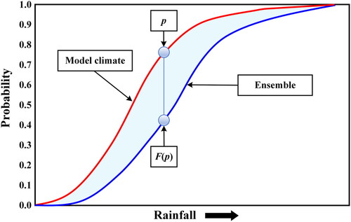
The EFI is a metric developed to assess the extremeness of a forecast by comparing its probability distribution with that of the model climate. It is computed as the difference between two cumulative distribution function (CDF) curves: one for the model climatological distribution obtained from the reforecasts, and the other for the current ensemble forecast distribution fitted with the daily ensemble members. The reforecasts and daily ensemble members are obtained from https://apps.ecmwf.int/datasets/. The frequency of occurrence of each value is used to estimate the probability distribution. The EFI is formulated by (1) $$\text{EFI}=\frac{2}{\pi }{\int }_0^1\frac{p-F(p)}{\sqrt{p(1-p)}}\mathit{\text{dp}}$$(1) where $p$ is the model climatological probability; $F(p)$ is the fraction of ensemble members that lie below the pth percentile of the model climate. One can visually estimate the EFI by assessing the area between model climate (red) and ensemble (blue) curves, as shown in Figure 1. The index values range from −1 to 1, where −1 denotes extremely low values and 1 denotes excessively high values for the model climate.

Figure 1. CDF curves of the model climatological and ensemble forecast.

2.2. Stacking ensemble learning model

For modeling and forecasting purposes, there has been a noticeable trend recently toward using ensemble learning approaches in numerous technical fields, such as hydrology. Bagging, Boosting, Stacking, and Blending are the most well-known and significant ensemble learning methodologies that have been developed and widely and successfully applied in hydrology and water resources. Stacking, in particular, is a widely used ensemble method that includes training multiple models and feeding their outputs as input features into a meta-model to make final predictions. As shown in Figure 2, we use the stacking ensemble learning framework to improve runoff prediction.

Figure 2. Illustration of the stacking ensemble learning framework.

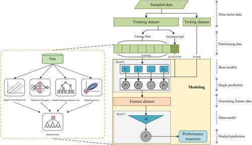
A stacking ensemble learning model’s architecture entails two or more base-models L_i and a meta-model M. The base-models, often referred to as level-0 models, are trained on a complete training dataset, then the meta-model, also referred to as a level-1 model, is built on the characteristics that are outputs of the base-models. The entire stacking ensemble learning process consists of seven steps.

1. The data is split into two parts, a training dataset, and a testing dataset. The training dataset is further divided into K-folds. In this study, the dataset is divided into five equally sized subsets.

2. A level-0 model is fitted on the K-1 parts and predictions are made for the Kth part.

3. This process is iterated until every fold has been predicted.

4. The level-0 model is then fitted on the whole training dataset to calculate its performance on the testing dataset.

5. Steps (b), (c), and (d) are repeated for other level-0 models.

6. Predictions from the training dataset are used as features for the level-1 model.

7. The level-1 model is used to predict the testing dataset.

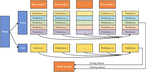
Given these, this study proposes a stacking ensemble learning strategy that combines predictions from multiple models using the same dataset, as shown in Figure 3.

Figure 3. Flowchart of the proposed stacking ensemble learning strategy.

In this study, we employ five distinct ML models to construct multiple regression models because they have all been used to analyze data from rainfall and runoff. The stacking ensemble learning model combines a meta-model (Random Forest) with four base-models: Ridge Regression, Gradient Boosting Decision Tree, Support Vector Regression, and Back Propagation, as depicted in Figure 2.

Here is a quick overview of these techniques and how they can be used to anticipate runoff.

• (1) Support Vector Regression (SVR)

Support Vector Regression, which can analyze regression data, is part of Support Vector Machines (SVM). SVR trains using a symmetrical loss function that equally penalizes high and low misestimates as a supervised learning method. Many researchers have used SVR to predict runoff (Hosseini and Mahjouri 2016; Liang et al. 2018; Xiang et al. 2018). The SVR model yields satisfactory accuracy and reliability at runoff prediction.

• (2) Multi-layer Perceptron (MLP)

A Multi-layer Perceptron is a name for a feed-forward and supervised artificial neural network, consisting of multiple layers of interconnected neurons, including an input layer, one or more hidden layers, and an output layer. It is trained using the back-propagation algorithm and is capable of handling both linearly separable and non-linearly separable data. For example, Riad selected MLP to model the rainfall-runoff relationship. The results indicated that the MLP model is more suitable to predict river runoff than classical regression model (Riad et al. 2004).

• (3) Gradient Boosting Decision Tree (GBDT)

A Gradient Boosting Decision Tree is a decision tree learning strategy that transforms numerous weak learners into strong learners. To minimize the loss function of the preceding model, such as mean square error or cross-entropy, each new model is trained to apply gradient descent. For example, Chen used GBDT to fit runoff from 22 event-based explanatory variables representing rainfall, soil moisture, groundwater level, and season (Chen et al. 2020).

• (4) Ridge Regression

Ridge regression is a method of estimating the coefficients of linear regression models when the independent variables are highly correlated. It performs the linear least squares function and L2 regularization, which reduces the variance and increases the bias of the coefficients. For example, Yu applied a ridge regression in a feature space. The proposed method provided higher accuracy on Tryggevælde catchment runoff and Mississippi River flow (Yu et al. 2020).

• (5) Random Forest (RF)

The random forest algorithm is an extension of the bagging method, which uses feature randomness except bagging to produce an uncorrelated forest of decision trees. Take the average of the individual decision trees for a regression task. The out-of-bag sample is then used for cross-validation, finalizing that prediction. RF has been used to predict runoff (Singh et al. 2022).

2.3. Particle swarm optimization algorithm

Kennedy and Eberhart created the population-based stochastic optimization method known as Particle Swarm Optimization (PSO) in the late twentieth century (Kennedy and Eberhart 1995). The social behavior of schooling fish or flocking birds served as its inspiration, where each member has a unique perceptual skill and modifies their behavior to the situation. In PSO, individuals are considered particles in a multidimensional search space, and every individual represents a potential answer to the optimization issue. The particle’s characteristics are described by its position, velocity, and fitness value, determined by the fitness function. During the process, particles autonomously adjust their distance and orientation depending on the ideal global fitness value, iteratively arriving at the best outcome.

Assume that a population of l particles exists in an N-dimensional space from a population $X=\{x_1,x_2,\dots ,x_l\},$ where $x_i=\left[\begin{array}{c}{x}_{i1},x_{i2},\dots ,x_{\mathit{\text{iN}}}\end{array}\right].$ The current properties of ith particle are expressed as (2) $$\begin{array}{c}\mathit{\text{Xi}}={(x_{i1}^t,x_{i2}^t,\dots ,x_{\mathit{\text{iN}}}^t)}^T\\ \mathit{\text{Vi}}={(v_{i1}^t,v_{i2}^t,\dots ,v_{\mathit{\text{iN}}}^t)}^T\\ \mathit{\text{Pi}}={(p_{i1}^t,p_{i2}^t,\dots ,p_{\mathit{\text{iN}}}^t)}^T\\ \mathit{\text{Pg}}={(p_{g1}^t,p_{g2}^t,\dots ,p_{\mathit{\text{gN}}}^t)}^T\end{array}$$(2) where $x_i^t$ is the current location at time t; $v_i^t$ is the current velocity at time t; $p_i^t$ is the best position in the histories of the particle at time t; $p_g^t$ is the best position in the histories of the entire particle swarm at time t.

Updates to the velocity and position are made by (3) $$\begin{array}{l}{v}_i^{t+1}=w{v}_i^t+c1r_1^t(p_i^t-x_i^t)+c2r_2^t(p_g^t-x_i^t)\\ x_i^{t+1}=x_i^t+v_i^{t+1}\end{array}$$(3) where $v_i^{t+1}$ and $x_i^{t+1}$ are the velocity and position at time t + 1, respectively; $c1$ and $c2$ constants that regulate the maximum step size in the range (0, 2), respectively; $r1$ and $r2$ are random values in the range (0, 1), respectively.

2.4. PSO-ML model

During the development of ML models, proper exploration of the hyperparameter space with optimization algorithms can find the ideal hyperparameters for the models. This paper builds a PSO-ML model for hyperparameter optimization, which combines the PSO method with the ML model to discover the best model structure over a range of lead times. The hyperparameters in each ML model are represented by an N-dimensional variable called the position of each particle. The positional information of each particle is initialized at random using the parameter’s range of values. Each particle’s ML model is configured separately, and the flow process is simulated. The Nash-Sutcliffe efficiency coefficient (NSE) of the results is defined as the particle fitness value. Each iteration aims to discover the maximum fitness value while updating particle position information. This is done until the maximum number of iterations is reached. Figure 4 depicts the structure of the PSO-ML model.

Figure 4. Flowchart of the PSO-ML model for hyperparameter optimization.

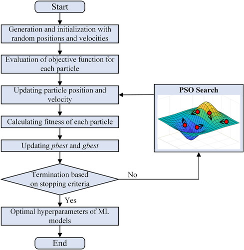
In order to find the optimal ML model structure, this study created a PSO-ML model for each ML model in level 0, including Support Vector Regression, Multi-layer Perceptron, Gradient Boosting Decision Tree, and Ridge Regression. Using the SVR model as an illustration, the data input to the SVR was in the form of a two-dimensional vector containing penalty factor and epsilon. The optimal hyperparameter combination was determined by selecting the hyperparameter combination that corresponds to the particle with the best fitness value in the particle swarm. Similarly, MLP, GBDT, and Ridge Regression also follow the above process. Given the complexity of hyperparameter selection during cross-validation, we combined the PSO algorithm separately with each ML model to obtain the optimal hyperparameter combination for all five folds.

2.5. Model setting and parameterization

Python 3.8 is the chosen programming language, and NumPy, Pandas, and PySwarms are the libraries used to prepare and manage our data. We employ the deep learning framework Google TensorFlow.

First, we preprocess the data required for the study to a format that can be understood by ML models. Second, the normalization operation is carried out. The process of normalization involves scaling data to fit within a specific range. Before feeding the selected rainfall (or EFI) and runoff time series into the adopted ML models, it is normalized to the range of [0, 1] for each of the 12 sub-areas by (4) $$\mathit{\text{Xnorm}}=\frac{X-X\mathrm{\text{min}}}{(X\mathrm{\text{max}}-X\mathrm{\text{min}})}$$(4) where $X\mathrm{\text{max}}$ and $X\mathrm{\text{min}}$ are the maximum and minimum value of each time series, respectively; $X$ is the value to be normalized, and $\mathit{\text{Xnorm}}$ is the normalized value of $X.$

Third, PSO algorithm’s parameters as well as the search parameter range have been set. The PSO algorithm’s inertial weight, learning factors, number of particles, and maximum number of iterations are parameters that require tuning and selection. These parameters directly impact the search effectiveness and convergence speed of the algorithm. To offer a sensible blend of parameters, the final choice was made according to the results of parameter setting by Xu (Xu et al. 2022). We chose 30 particles and 200 iterations as the number of particles and the maximum number of iterations, respectively; 0.8 for the inertial weight $w;$ 2 for the sum of the learning factors $c1$ and $c2.$

According to the features of the rainfall (or EFI) and runoff time series data, the hyperparameters and optimization ranges in each model are set in Table 1. Using the MLP model as an illustration, batch size defines the number of samples we use in one epoch to train a neural network, and selecting an appropriate batch size can enhance the speed and stability of model training. Learning rate refers to the rate at which an algorithm converges to a solution, dictating the degree to which the model adjusts its parameters along the gradient during each iteration. Number of cells pertains to the quantity of neurons present in the hidden layer, serving as an indicator of the complexity of the MLP network and its capacity to capture data features. The optimization ranges for the three hyperparameters are as follows: the batch size varies uniformly over the integer range of 24–128, while the learning rate and number of cells are chosen uniformly from the ranges of [0, 1] and [8, 64], respectively.

Table 1. Model hyperparameter setting.

Model	Hyperparameter	Optimization range
SVR	Penalty factor	[0, 5]
	Epsilon	[0, 1]
MLP	Batch size	[24, 128]
	Learning rate	[0, 1]
	Number of cells	[8, 64]
GBDT	N_estimators	[100, 300]
	Learning rate	[0, 1]
	Max_depth	[2, 8]
Ridge regression	Alpha	[0, 200]

2.6. Performance evaluation criteria

In this study, the performance of different models is evaluated by statistical error measures, including the relative flood peak error (RPE), mean relative error (MRE), root mean square error (RMSE), Nash-Sutcliffe efficiency coefficient (NSE), and Coefficient Persistence (CP). Unlike conventional assessment metrics such as RPE, RMSE, and MAE, Nash-Sutcliffe efficiency coefficient (NSE) is a hydrological indicator used to assess the degree of agreement between the hydrological model simulation results and the observed data. The NSE value ranges from minus infinity to 1, with values closer to 1 indicating a better match between the model simulation results and the observed data. Furthermore, a more appropriate index for evaluating the accuracy of model outputs is Coefficient Persistence (CP), which is specifically designed for real-time runoff forecasting (Kitanidis and Bras 1980). Reference values for the RPE, RMSE, MAE, and NSE results are described in Table 2 (Markuna et al. 2023; Mirzania et al. 2023; Vishwakarma et al. 2023b). These metrics’ mathematical expressions can be described by (5) $$\begin{array}{l}\mathit{\text{RPE}}=\frac{\left|Q_s^p-Q_o^p\right|}{Q_o^p}\mathrm{\times }100\%\\ \mathit{\text{MRE}}=\frac{1}{T}\sum _{t=1}^T\frac{\left|Q_s^t-Q_o^t\right|}{Q_o^t}\times 100\%\\ \mathit{\text{RMSE}}=\sqrt{\frac{1}{T}\sum _{t=1}^T{(Q_s^t-Q_o^t)}^2}\\ \mathit{\text{NSE}}=1-\frac{\sum _{t=1}^T{(Q_s^t-Q_o^t)}^2}{\sum _{t=1}^T{(Q_o^t-{\overline{Q}}_o)}^2}\\ \mathit{\text{CP}}(i)=1-\frac{\sum _{t=1}^T{(Q_s^t-Q_o^t)}^2}{\sum _{t=1}^T{(Q_o^t-Q_o^{t-i})}^2}\end{array}$$(5) where $Q_o^p$ and $Q_s^p$ is the observed and simulated flood peak discharge, respectively; $Q_o^t$ and $Q_s^t$ are observed and simulated runoff at time t, respectively; ${\overline{Q}}_o$ is the mean of observed runoff; $Q_o^{t-i}$ is observed runoff at time (t-i).

Table 2. The characteristics of acceptable results for RPE, RMSE, MAE, and NSE.

Performance rating	RPE (%)	MRE (%)	RMSE (m^3/s)	NSE
Very good	0≤RPE ≤ 10	0≤MRE ≤ 10	0≤RMSE ≤ 700	0.75<NSE ≤ 1.00
Good	10<RPE ≤ 25	10<MRE ≤ 25	700<RMSE ≤ 850	0.65<NSE ≤ 0.75
Satisfactory	25<RPE ≤ 40	25<MRE ≤ 40	850<RMSE ≤ 1000	0.50<NSE ≤ 0.65
Unsatisfactory	RPE > 40	MRE > 40	RMSE > 1000	NSE ≤ 0.50

3. Case study

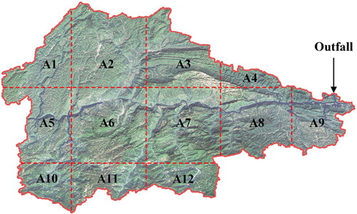
The study region is situated in the Qing River, which is the first major tributary of the Yangtze River downstream from the Three Gorges, in the Hubei province of China. The Qing River Basin features a moderate climate, an average annual rainfall of approximately 1,400 mm, and an average flow of 440 m³/s. The amount of rain that falls here varies greatly throughout the year, with the majority falling between April and October, accounting for 87% of the total annual rainfall. This basin is part of the cascade hydropower development in the Yangtze River, with Gaobazhou, Geheyan, and Shuibuya serving as the main reservoirs that cooperate in real-time flood control. Therefore, comprehending and predicting the rainfall-runoff dynamics in the region is crucial for hydropower development and flood prevention. In this study, we select a representative area (110°0′0″-30°47′15″, 30°3′21″-111°13′27″) upstream of the Geheyan Reservoir as our study location, divided into 12 sub-areas denoted as A1 to A12, as shown in Figures 5 and 6.

Figure 5. Sub-area divisions in the study area.

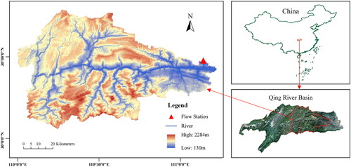
Figure 6. Daily inflow of the Geheyan Reservoir.

The data used in the study include the local rainfall, EFI, and runoff data.

• (1) Rainfall and EFI data

ECMWF plays a crucial role in generating global numerical weather predictions and providing related data to Member and Co-operating States, as well as the wider community. The ECMWF Integrated Forecasting System ensemble, consisting of the control and 50 perturbed members (spanning up to 15 days), is accessed from the ECMWF Meteorological Archival and Retrieval System. To compare the current ensemble forecasts with a model climate, ECMWF generates reforecasts using an 11-member ensemble of 46-day ENS integrations that start on the same day and month as each real-time prediction for the last 20 years. These reforecasts are based on a 4-week timeframe (9 start dates x 20 years x 11 members = 1980 integrations), centered around the forecast’s data time. In this study, daily total surface precipitation control forecasts, ensemble forecasts, and reforecasts from ECMWF are used to obtain rainfall and EFI data. The data spans from 2015/01/01 to 2020/12/31 (a total of 2,192 days). The focus is primarily on forecasts up to 72 h ahead, with three lead times (24, 48, and 72 h), and a grid resolution of 0.25° × 0.25°.

• (2) Runoff data

Runoff data used in this study is the historical daily inflow of the Geheyan Reservoir, from 2015/01/01 to 2020/12/31 (a total of 2,192 days) commensurately.

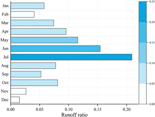
In ML, the dependability of model training can be increased by selecting a small, representative dataset from a large population. Therefore, it is necessary to select representative datasets from the whole time series. By investigating the historical daily inflow of the Geheyan Reservoir, from 2015/01/01 to 2020/12/31, it is found that the monthly runoff looks like regular behaviors over a generally fixed period. A representative time series is constructed based on the original time series by selecting the months with high runoff. Figure 7 illustrates the daily inflow of the Geheyan Reservoir from January 1st, 2015 to December 31st, 2020, encompassing a total of 2,192 days. Based on this data, the monthly runoff ratio of the total annual runoff is calculated, as shown in Figure 8. Consequently, the time series for our study consists of the daily rainfall and EFI data from May to July for the years 2015–2020, totaling 552 days.

Figure 7. Daily inflow of the Geheyan Reservoir.

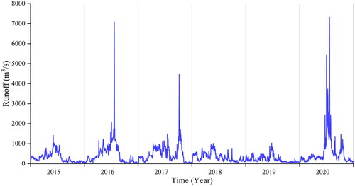
Figure 8. Monthly runoff ratio of the total annual runoff.

Data splitting is a crucial aspect of data science when creating models based on data. For the runoff prediction in this study, we selected the rainfall (or EFI) and runoff time series from May to July 2015–2020 (552 days in total). We used the rainfall (or EFI) time series of the 12 sub-areas and antecedent runoff time series of the Geheyan Reservoir to forecast runoff with three lead times, including 24, 48, and 72 h, with a spatial resolution of 0.25° × 0.25°. The time series was split into two parts: a training dataset and a testing dataset. Table 3 and Table 4 illustrate the summary of data samples in the training and testing dataset through their statistical values, respectively. R₂₄, R₄₈, R₇₂ are the rainfall time series with 24, 48, and 72 h lead times, respectively; EFI₂₄, EFI₄₈, EFI₇₂ are the EFI time series with 24, 48, and 72h lead times, respectively; Q_t is the antecedent runoff time series, with the one day antecedent, two day antecedent, and three day antecedent runoff time series; Q₁, Q₂, and Q₃ are the one-day-ahead, two-day-ahead, and three-day-ahead runoff time series, respectively; S₁, S₂, and S₃ are the simulated runoff time series of Q₁, Q₂, and Q₃, respectively.

Table 3. Summary of the training dataset (count = 460).

Lead time (h)	Timespan	Input	Output
24	May to July 2015–2019	R24 (or EFI24), Qt, and Q1	S1
48	May to July 2015–2019	R48 (or EFI48), Qt, and Q2	S2
72	May to July 2015–2019	R72 (or EFI72), Qt, and Q3	S3

Table 4. Summary of the testing dataset (count = 92).

Lead time (h)	Timespan	Input	Output
24	May to July 2020	R24 (or EFI24), Qt, and Q1	S1
48	May to July 2020	R48 (or EFI48), Qt, and Q2	S2
72	May to July 2020	R72 (or EFI72), Qt, and Q3	S3

4. Results and discussion

4.1. EFI calculation and feature

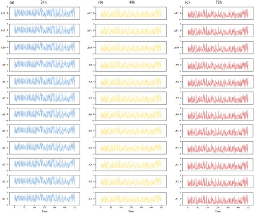
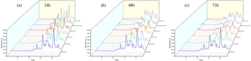
For each of 12 sub-areas, 50 ensemble forecasts and reforecasts were used to calculate EFI values with different lead times. The calculated EFI time series were fed into the further hydrological models, as shown in Figure 9. The EFI is founded on the hypothesis that if the forecast rainfall is extreme and relative to the model climate, then the actual rainfall would be an extreme event relative to the actual rainfall. The EFI is free of model bias because it makes use of the same model reforecast dataset. Additionally, it is a useful tool for areas with little observations. Compared to rainfall, EFI may have a stronger potential to be applied for accurate runoff prediction.

Figure 9. EFI values of 12 sub-areas with different lead times.

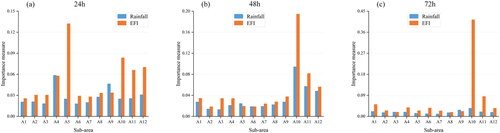
To evaluate the importance of input features on the runoff results, rainfall and EFI time series of 12 sub-areas are feeding into Random Forest (RF) framework in the study. RF method is capable of analyzing input features of complex interactions, whose variable importance measures can be used as feature selection tools for high-dimensional data. To more intuitively see how input features affect the runoff results, the importance measure of each input feature in the RF model to the predicted runoff in different lead times are shown in Figure 10. For all lead times, among most sub-areas, EFI importance measures are higher than rainfall importance measures. It is concluded that the importance of rainfall inputs is more significant than that of EFI inputs, which means that the EFI has a higher precedence in terms of runoff physical causes.

Figure 10. Importance measures with different lead times.

4.2. PSO-ML model optimization

The ML hyperparameter combination with the best prediction effect was discovered following PSO algorithm iterations. Tables 5 and 6 illustrate the hyperparameter optimization at different lead times (24, 48, and 72 h) in rainfall-runoff and EFI-runoff simulation, respectively. The experiment that comes after applies the results of hyperparameter optimization into further hydrological modelling.

Table 5. Optimal PSO-ML hyperparameters for different lead times in rainfall-runoff simulation.

	Lead time (h)	Penalty factor		Epsilon
SVR	24	3.033		0.182
	48	2.978		0.246
	72	1.019		0.224
MLP	Lead time (h)	Batch size	Learning rate	Number of cells
	24	64	0.090	15
	48	56	0.071	10
	72	62	0.157	19
GBDT	Lead time (h)	N_estimators	Learning rate	Max_depth
	24	126	0.048	3
	48	147	0.057	2
	72	131	0.063	2
Ridge Regression	Lead time (h)	Alpha
	24	0.114
	48	104.772
	72	95.085

Table 6. Optimal PSO-ML hyperparameters for different lead times in EFI-runoff simulation.

	Lead time (h)	Penalty factor		Epsilon
SVR	24	2.257		0.122
	48	2.926		0.025
	72	2.978		0.122
MLP	Lead time (h)	Batch size	Learning rate	Number of cells
	24	54	0.061	34
	48	58	0.289	25
	72	60	0.115	24
GBDT	Lead time (h)	N_estimators	Learning rate	Max_depth
	24	132	0.079	3
	48	169	0.053	3
	72	143	0.052	4
Ridge Regression	Lead time (h)	Alpha
	24	2.501
	48	120.629
	72	146.616

4.3. Comparisons of prediction results between rainfall-runoff and EFI-runoff simulation

For the runoff prediction experiment in our study area, we prepared the datasets for the SVR, MLP, GBDT, Ridge Regression, and stacking models by setting the input rainfall (or EFI) time series. To achieve this, we split the time series required for the study into two parts, which can be recognized by ML models. Next, we used the PSO algorithm to optimize the model hyperparameters, improving the models’ ability to learn the time series features. Finally, to make our research more convincing, we used four indexes to measure the performance of the different models for runoff prediction. The SVR, MLP, GBDT, and Ridge Regression were used for comparison purposes.

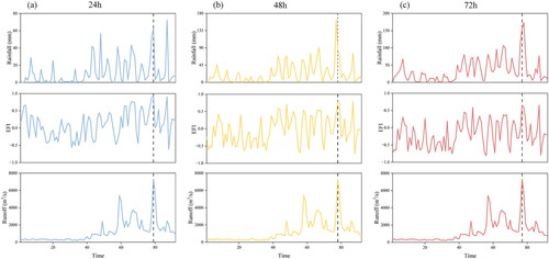
Before feeding the rainfall (or EFI) and runoff time series into hydrological models, the average rainfall, average EFI, and runoff time series on the held-out testing samples were compared in Figure 11. For one-day-ahead prediction, the flood peak moment corresponds to the maximum EFI value, with the maximum rainfall moment is much later than the flood peak. For two-day-ahead prediction, the flood peak moment corresponds to the maximum EFI value, with the maximum rainfall moment is slightly earlier than the flood peak. For one-day-ahead prediction, the flood peak moment corresponds to the maximum EFI value; with the maximum rainfall moment is slightly later than the flood peak. For flood peak prediction with different lead times, it can be seen that the EFI-runoff relationship is superior to the rainfall-runoff relationship. Therefore, EFI-runoff simulation may show more significant forecasting skills than rainfall-runoff simulation.

Figure 11. Rainfall, EFI, and runoff time series on the held-out testing samples with different lead times.

Based on the results of hyperparameter optimization, comparisons were made between rainfall-runoff and EFI-runoff simulation with 24, 48, and 72 h lead times. Multiple models were simulated, and the results were shown in Figure 12. It can be seen that the accuracy of EFI-runoff simulation is slightly better than that of rainfall-runoff simulation for different models and lead times. To make a more detailed comparison, four evaluation indices, including the RPE, MRE, RMSE, and NSE, were calculated and listed in Table 7.

Figure 12. Multiple model prediction results on the held-out testing samples obtained by two inputs with different lead times.

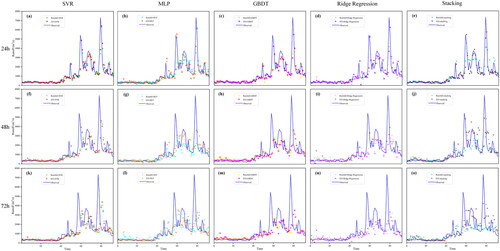
Table 7. Evaluation indices comparison of two inputs.

Lead time (h)	Model	Input factor	RPE (%)	MRE (%)	RMSE (m^3/s)	NSE	CP(1)
24	SVR	Rainfall	13.686	24.785	766.816	0.663	0.230
		EFI	12.398	23.993	765.526	0.672	0.250
	MLP	Rainfall	16.854	27.580	720.129	0.703	0.321
		EFI	15.473	25.790	718.202	0.705	0.324
	GBDT	Rainfall	25.764	29.531	784.226	0.648	0.210
		EFI	25.178	27.418	768.305	0.662	0.194
	Ridge Regression	Rainfall	14.268	31.558	758.620	0.671	0.245
		EFI	13.483	28.724	739.692	0.687	0.285
	Stacking	Rainfall	8.588	26.293	655.775	0.754	0.394
		EFI	7.987	22.421	632.871	0.771	0.496
48	SVR	Rainfall	39.357	34.330	1123.982	0.274	−0.654
		EFI	37.083	32.756	1114.051	0.287	−0.625
	MLP	Rainfall	52.793	36.945	1058.311	0.356	−0.466
		EFI	51.158	35.607	920.534	0.513	−0.107
	GBDT	Rainfall	51.890	39.233	1095.381	0.310	−0.571
		EFI	50.564	37.337	1065.885	0.347	−0.488
	Ridge Regression	Rainfall	48.027	40.355	1049.873	0.366	−0.444
		EFI	46.799	38.470	1010.632	0.413	−0.338
	Stacking	Rainfall	34.087	33.697	1021.549	0.400	−0.366
		EFI	33.473	32.157	807.007	0.626	0.149
72	SVR	Rainfall	44.510	42.570	1235.040	0.120	−0.997
		EFI	39.867	38.584	1196.178	0.174	−0.874
	MLP	Rainfall	55.559	45.778	1145.035	0.243	−0.713
		EFI	51.740	37.407	994.286	0.429	−0.294
	GBDT	Rainfall	53.982	42.975	1204.416	0.163	−0.899
		EFI	52.511	40.805	1119.240	0.277	−0.641
	Ridge Regression	Rainfall	56.402	45.004	1169.941	0.210	−0.792
		EFI	54.990	43.133	1080.041	0.327	−0.528
	Stacking	Rainfall	43.953	41.901	1111.053	0.287	−0.616
		EFI	42.693	36.710	940.715	0.489	−0.158

The EFI-runoff simulation is more accurate for five models across all lead times. With extended lead times, the forecast accuracy of all models decreases to varying degrees, but the stacking model maintains high prediction levels. These results confirm that the EFI-based stacking model established has a consistently positive effect in flood process simulation. However, the experiment’s limitation is that it does not demonstrate whether the stacking model is more efficient than the last known observed information.

Table 7 reveals that introducing EFI as a model input has improved all four evaluation indices of multiple models. For instance, for one-day-ahead prediction results of the SVR model, the relative flood peak error, mean relative error, root mean square error, and Nash-Sutcliffe efficiency coefficient with rainfall-runoff simulation are 13.686%, 24.785%, 766.816 m³/s, and 0.663, respectively, while those with EFI-runoff simulation are 12.398%, 23.993%, 765.526 m³/s, and 0.672, respectively. Additionally, for one-day-ahead prediction results of the stacking model, four evaluation indices with rainfall-runoff simulation are 8.588%, 26.293%, 655.775 m³/s, and 0.754, respectively, while those with EFI-runoff simulation are 7.987%, 22.421%, 632.871 m³/s, and 0.771, respectively. For all hydrological models and lead times, it can be seen from Table 7 that the performances of EFI-runoff simulation are better than those of rainfall-runoff simulation. In this experiment, we calculate the CP of all models across various lead times. A CP value closer to 1 indicates higher stability and consistency of the process or system under consideration. It shows that in most cases, the EFI runoff simulation exhibits a higher CP value, indirectly affirming the effectiveness of EFI as an input factor for runoff prediction. It is evident that the evaluation indices for the SVR, MLP, and GBDT, Ridge Regression, and stacking models are substantially improved with EFI-runoff simulation. These findings demonstrate that EFI-runoff simulation can enhance the capability of runoff prediction, because EFI is more sensitive to the observed runoff.

Referring to Table 2 for the acceptable results characteristics of RPE, RMSE, MAE, and NSE, we compare the quality of four individual models for rainfall-runoff simulation and EFI-runoff simulation. For instance, for two-day-ahead prediction results of the MLP model, the relative flood peak error, mean relative error, root mean square error, and Nash-Sutcliffe efficiency coefficient with rainfall-runoff simulation are considered ‘unsatisfactory’, ‘satisfactory’, ‘unsatisfactory’, and ‘unsatisfactory’, while those with EFI-runoff simulation are considered ‘unsatisfactory’, ‘satisfactory’, ‘satisfactory’, and ‘satisfactory’, respectively. It can be seen from the acceptable results that the prediction effect of EFI-runoff simulation is significantly better than rainfall-runoff simulation. The acceptable results for the PRE and MRE indicators appear to be the same, but EFI-runoff simulation displays a 3.10% lower PRE, and 3.62% lower MRE. In summary, EFI-runoff simulation is able to provide high-precision runoff results compared with rainfall-runoff simulation. Hence, it should be implemented for real-time runoff prediction.

4.4. Comparisons of prediction results between stacking and individual model

Based on the above results, EFI was introduced as a model input to enhance runoff prediction in further experiments. For EFI-runoff simulation, the prediction results of multiple models with different lead times (24, 48, and 72 h) were compared, as shown in Figure 13. For all lead times, it can be seen that the accuracy of the stacking model is better than that of other individual models. To demonstrate the performances of different models more visually, Figure 13 gives the comparison of the evaluation index using different hydrological models for continuous flow processes with 24, 48, and 72 h lead times.

Figure 13. Comparisons of multiple model prediction results on the held-out testing samples with different lead times.

From the results presented in Figure 14, it is evident that the stacking model outperforms other models in terms of all four evaluation indices. For instance, the one-day-ahead prediction results of the stacking model show the relative flood peak error, mean relative error, root mean square error, Nash-Sutcliffe efficiency coefficient, and coefficient persistence of 7.987%, 22.421%, 632.871 m³/s, 0.771, and 0.469, respectively, which is better than the results obtained from the SVR, MLP, GBDT, and Ridge Regression model. The two-day-ahead and three-day-ahead prediction results are also similar. Furthermore, the prediction accuracy decreases as the lead time lengthens. The model performs better with 24 h lead time than 48 h lead time, and 48 h lead time performs better than 72 h lead time.

Figure 14. Four evaluation indices of the predictions using the SVR, BP, GBDT, Ridge Regression, and stacking model for different lead times.

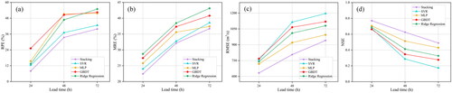
Referring to Table 2 for the acceptable results characteristics, we compare the quality of four individual models and the stacking model for EFI runoff simulation. For instance, for two-day-ahead prediction results, the RMSE obtained from the stacking model is considered ‘good’, while those obtained from the SVR, MLP, GBDT, Ridge Regression models are considered ‘unsatisfactory’, ‘satisfactory’, ‘unsatisfactory’, and ‘unsatisfactory’, respectively. The acceptable results demonstrate that the stacking method has a significantly better prediction effect than individual models. In summary, the stacking model can offer a reasonable and robust prediction result compared with other models.

4.5. Discussion

This study introduces a novel driving factor into runoff prediction: the EFI, derived from both model climatological and ensemble forecast. Results demonstrate that the EFI-based stacking model outperforms other models, highlighting the efficacy of this approach. Currently, runoff prediction studies predominantly hinge on historical rainfall and runoff records, alongside future rainfall forecast data. However, these inputs may not fully capture the trend of future runoff, leading to constrained accuracy enhancements. Acquiring measured rainfall data can be challenging, particularly in data-scarce regions. Therefore, leveraging climate models to predict future rainfall becomes a viable alternative for data acquisition. Following our research, we have discovered that the EFI-runoff simulation can improve runoff prediction capability due to EFI’s higher sensitivity to observed runoff. Our experiments address the challenges of acquiring input data and enhancing accuracy in data-scarce regions effectively. The method proposed has the potential to be extended to any region with historical inflow data, making it widely applicable across diverse geographical areas. Compared to individual models or traditional precipitation-runoff models, the proposed method exhibits significantly enhanced accuracy. This improvement aligns well with the practical requirements of various projects to a considerable extent.

The limitations of the experiment include the observation that although the proposed method enhances prediction results, its effectiveness with different lead times remains suboptimal. Additionally, the model algorithm does not involve recurrent neural networks, which are better suited for handling dynamic and sequential data. Future research will focus on incorporating more advanced networks to conduct deeper explorations in this regard. In summary, this paper proposes a method that provides innovative insights and holds considerable potential for predicting runoff across large-scale areas.

5. Conclusion

This study introduces EFI as a model input to the SVR, MLP, GBDT, Ridge Regression, and stacking models for runoff prediction with lead times of 24, 48, and 72 h. Additionally, the study proposes and tests the stacking ensemble approach, optimizes model hyperparameters using the PSO algorithm, and compares model performances under various conditions. The approach focuses on predicting the inflow processes of the Geheyan Reservoir in the Qing River. Results of the study indicate that EFI-runoff simulation shows significant forecasting skills and can improve the runoff prediction capability compared to rainfall-runoff simulation. Furthermore, the proposed stacking model outperforms the SVR, MLP, GBDT, and Ridge Regression in terms of the relative flood peak error, mean relative error, root mean square error, and Nash-Sutcliffe efficiency coefficient for all lead times. Meanwhile, the accuracy of runoff prediction decreases with an increase in lead time. Overall, the study suggests that the extreme forecast index-driven runoff prediction approach using stacking ensemble learning has the potential to be applied for accurate runoff prediction.

Given that this is the first attempt to introduce EFI to solve runoff prediction problems, the experiment’s limitation is that it cannot demonstrate whether the stacking model is more efficient than the last known observed information. The proposed EFI-based stacking model does not adequately account for temporal and spatial correlations. In future research, more advanced deep learning models are expected to be proposed for runoff prediction challenges.

Nomenclature
EFI	=	extreme forecast index
CDF	=	cumulative distribution function
PSO	=	particle swarm optimization
ML	=	machine learning
SVR	=	support vector regression
MLP	=	multi-layer perceptron
GBDT	=	gradient boosting decision
ECMWF	=	European center for medium-range weather forecasts
GBDT	=	gradient boosting decision
RF	=	random forest
ML	=	machine learning
RPE	=	relative flood peak error
MRE	=	mean relative error
RMSE	=	root mean square error
NSE	=	Nash-Sutcliffe efficiency coefficient
CP	=	coefficient persistence

Author contributions

Zhiyuan Leng: Writing - original draft, Conceptualization, Methodology, Software, Data curation. Lu Chen: Writing - review & editing, Conceptualization, Investigation, Supervision, Project management, Funding acquisition. Binlin Yang: Methodology, Data curation. Siming Li: Methodology, Data curation. Bin Yi: Methodology, Data curation.

Data availability statement

Data will be made available on request.

Disclosure statement

No conflict of interest exits in the submission of this manuscript, and manuscript is approved by all authors for publication.

Additional information

Funding

This research was supported by the National Key R&D Program of China (2023YFC3081000), the Science and Technology Plan Projects of Tibet Autonomous Region (XZ202301YD0044C).

References

- Achite M, Elshaboury N, Jehanzaib M, Vishwakarma D, Pham Q, Anh D, Abdelkader E, Elbeltagi A.,. 2023. Performance of machine learning techniques for meteorological drought forecasting in the Wadi Mina Basin, Algeria. Water. 15(4):765. doi: 10.3390/w15040765.
- Agarwal A, Singh RD. 2004. Runoff modelling through back propagation artificial neural network with variable rainfall-runoff data. Water Resour Manage. 18:285–300.
- Akhter T, Pandit BA, Vishwakarma DK, Kumar R, Mishra R, Maryam M.,. 2022. Meteorological drought quantification using standardized precipitation index for Gulmarg area of Jammu and Kashmir. J Soil Water Conserv. 21(3):260–267. doi: 10.5958/2455-7145.2022.00033.9.
- Bougeault P, Toth Z, Bishop C, et al. 2010. The THORPEX Interactive Grand Global Ensemble. B Am Meteorol Soc. 91(8):1059–1072.
- Chen X, Parajka J, Széles B, Strauss P, Blöschl G. 2020. Controls on event runoff coefficients and recession coefficients for different runoff generation mechanisms identified by three regression methods. J Hydrol Hydromech. 68(2):155–169. doi: 10.2478/johh-2020-0008.
- Elbeltagi A, Kumar M, Kushwaha NL, Pande CB, Ditthakit P, Vishwakarma DK, Subeesh A.,. 2023a. Drought indicator analysis and forecasting using data driven models: case study in Jaisalmer, India. Stoch Environ Res Risk Assess. 37(1):113–131. doi: 10.1007/s00477-022-02277-0.
- Elbeltagi A, Pande CB, Kumar M, Tolche AD, Singh SK, Kumar A, Vishwakarma DK.,. 2023b. Prediction of meteorological drought and standardized precipitation index based on the random forest (RF), random tree (RT), and Gaussian process regression (GPR) models. Environ Sci Pollut Res Int. 30(15):43183–43202. doi: 10.1007/s11356-023-25221-3.
- Emerton RE, Stephens EM, Pappenberger F, et al. 2016. Continental and global scale flood forecasting systems. Wiley Interdiscip Rev Water. 3(3):391–418.
- Fernández-Delgado M, Cernadas E, Barro S, et al. 2014. Do we need hundreds of classifiers to solve real world classification problems? J Mach Learn Res. 15(1):3133–3181.
- Hosseini SM, Mahjouri N. 2016. Integrating support vector regression and a geomorphologic artificial neural network for daily rainfall-runoff modeling. Appl Soft Comput. 38:329–345.
- Inoue J. 2020. Review of forecast skills for weather and sea ice in supporting Arctic navigation. Polar Sci. 27:100523. doi: 10.1016/j.polar.2020.100523.
- Kennedy J, Eberhart R. 1995. Particle swarm optimization//Proceedings of ICNN’95-international conference on neural networks. IEEE. 4, p. 1942–1948.
- Kimuli JB, Di B, Zhang R, et al. 2021. A multisource trend analysis of floods in Asia-Pacific 1990-2018: implications for climate change in sustainable development goals. Int J Disaster Risk Reduct. 59(5):102237.
- Kitanidis PK, Bras RL. 1980. Real-time forecasting with a conceptual hydrologic model: 2. Applications and results. Water Resour Res. 16(6):1034–1044.
- Kumar D, Singh VK, Abed SA, Tripathi VK, Gupta S, Al-Ansari N, Vishwakarma DK, Dewidar AZ, Al‑Othman AA, Mattar MA, et al. 2023. Multi-ahead electrical conductivity forecasting of surface water based on machine learning algorithms. Appl Water Sci. 13(10):192. doi: 10.1007/s13201-023-02005-1.
- Lalaurette F. 2003. Early detection of abnormal weather conditions using a probabilistic extreme forecast index. QJR Meteorol Soc. 129(594):3037–3057.
- Liang Z, Li Y, Hu Y, Li B, Wang J. 2018. A data-driven SVR model for long-term runoff prediction and uncertainty analysis based on the Bayesian framework. Theor Appl Climatol. 133(1-2):137–149.,. doi: 10.1007/s00704-017-2186-6.
- Markuna S, Kumar P, Ali R, et al. 2023. Application of innovative machine learning techniques for long-term rainfall prediction. Pure Appl Geophys. 180(1):335–363.
- Mirzania E, Vishwakarma DK, Bui Q-AT, Band SS, Dehghani R.,. 2023. A novel hybrid AIG-SVR model for estimating daily reference evapotranspiration. Arab J Geosci. 16(5):1–14. doi: 10.1007/s12517-023-11387-0.
- Mosavi A, Ozturk P, Chau K. 2018. Flood prediction using machine learning models: literature review. Water. 10(11):1536. doi: 10.3390/w10111536.
- Pedregosa F. 2016. Hyperparameter optimization with approximate gradient//International conference on machine learning. PMLR. p. 737–746.
- Prates F, Buizza R. 2011. PRET, the Probability of RETurn: a new probabilistic product based on generalized extreme-value theory. QJR Meteorol Soc. 137(655):521–537.
- Rajaee T, Khani S, Ravansalar M. 2020. Artificial intelligence-based single and hybrid models for prediction of water quality in rivers: a review. Chemom Intell Lab Syst. 200:103978.
- Riad S, Mania J, Bouchaou L, et al. 2004. Rainfall-runoff model using an artificial neural network approach. Math Comput Model. 40(7-8):839–846.
- Saha A, Pal S, Arabameri A, Blaschke T, Panahi S, Chowdhuri I, Chakrabortty R, Costache R, Arora A.,. 2021. Flood susceptibility assessment using novel ensemble of hyperpipes and support vector regression algorithms. Water. 13(2):241. doi: 10.3390/w13020241.
- Sahoo BB, Jha R, Singh A, Kumar D.,. 2019. Long short-term memory (LSTM) recurrent neural network for low-flow hydrological time series forecasting. Acta Geophys. 67(5):1471–1481. doi: 10.1007/s11600-019-00330-1.
- Singh AK, Kumar P, Ali R, Al-Ansari N, Vishwakarma DK, Kushwaha KS, Panda KC, Sagar A, Mirzania E, Elbeltagi A, et al. 2022. An integrated statistical-machine learning approach for runoff prediction. Sustainability. 14(13):8209. doi: 10.3390/su14138209.
- Sudriani Y, Ridwansyah I, Rustini HA. 2019. Long short term memory (LSTM) recurrent neural network (RNN) for discharge level prediction and forecast in Cimandiri river, Indonesia//IOP Conference Series: earth and Environmental Science. IOP Conf Ser Earth Environ Sci. 299(1):012037. doi: 10.1088/1755-1315/299/1/012037.
- Sun W, Trevor B. 2018. A stacking ensemble learning framework for annual river ice breakup dates. J Hydrol. 561:636–650.
- Todini E. 2007. Hydrological catchment modelling: past, present and future. Hydrol Earth Syst Sci. 11(1):468–482.
- Tsonevsky I, Doswell CA, Brooks HE. 2018. Early warnings of severe convection using the ECMWF extreme forecast index. Weather Forecast. 33(3):857–871. doi: 10.1175/WAF-D-18-0030.1.
- Vishwakarma DK, Kumar R, Abed SA, Al-Ansari N, Kumar A, Kushwaha NL, Yadav D, Kumawat A, Kuriqi A, Alataway A, et al. 2023b. Modeling of soil moisture movement and wetting behavior under point-source trickle irrigation. Sci Rep. 13(1):14981. doi: 10.1038/s41598-023-41435-4.
- Vishwakarma DK, Kuriqi A, Abed SA, Kishore G, Al-Ansari N, Pandey K, Kumar P, Kushwaha NL, Jewel A.,. 2023a. Forecasting of stage-discharge in a non-perennial river using machine learning with gamma test. Heliyon. 9(5):e16290. doi: 10.1016/j.heliyon.2023.e16290.
- Wu Z, Zhou Y, Wang H, Jiang Z.,. 2020. Depth prediction of urban flood under different rainfall return periods based on deep learning and data warehouse. Sci Total Environ. 716:137077. doi: 10.1016/j.scitotenv.2020.137077.
- Xiang Y, Gou L, He L, et al. 2018. A SVR-ANN combined model based on ensemble EMD for rainfall prediction. Appl Soft Comput. 73:874–883.
- Xu Y, Hu C, Wu Q, et al. 2022. Research on particle swarm optimization in LSTM neural networks for rainfall-runoff simulation. J Hydrol. 608:127553.
- Yang B, Chen L, Singh VP, Yi B, Leng Z, Zheng J, Song Q. 2023. A method for monthly extreme precipitation forecasting with physical explanations. Water. 15(8):1545. doi: 10.3390/w15081545.
- Yu X, Liong SY. 2007. Forecasting of hydrologic time series with ridge regression in feature space. J Hydrol. 332(3–4):290–302.
- Yu X, Wang Y, Wu L, et al. 2020. Comparison of support vector regression and extreme gradient boosting for decomposition-based data-driven 10-day streamflow forecasting. J Hydrol. 582:124293.
- Zhou Z. 2009. Ensemble learning. Encycl Biometr. 1
- Zounemat-Kermani M, Batelaan O, Fadaee M, et al. 2021. Ensemble machine learning paradigms in hydrology: a review. J Hydrol. 598:126266.
- Zsótér E. 2006. Recent developments in extreme weather forecasting. ECMWF Newsl. 107(107):8–17.