Decadal-scale assessment of sediment denudation rates in the Zhoukou River Basin, Taiwan: insights from improved DEMs of differencing based on spectral analysis

Abstract

This study assesses sediment erosion rates in the Zhoukou River Basin in southern Taiwan over the past three decades, focusing on the impact of extreme rainfall events. While various established methods determine erosion rates over different temporal scales, we employ an independent approach for decadal-scale erosion rate calculation by utilizing open-source global and regional digital elevation models (DEMs) data for two distinct periods. We introduce a new method that applies Fourier analysis to vertically register the DEMs, significantly minimizing their vertical bias. Through spectral analysis, we identify long wavelength topography crucial for correcting vertical offsets. Erosion rates, computed through DEMs of Difference (DoD), exhibit a similar trend of significant reduction in sediment export rates from 1990–2010 to 2011–2020 due to decreased extreme rainfall events, aligning with erosion rate estimates derived from mean suspended load data at gauge stations. Over the entire period from 1990 to 2020, the calculated denudation rate was 14.19 mm/yr, whereas in the recent decade (2011–2020), it decreased to 10.46 mm/yr. Our study suggests that the improved DoD method can effectively estimate sediment transport rates by leveraging underutilized DEMs captured at distinct points in time, especially when the erosional signal dominates data noise.

Keywords:

• DEMs of difference (DoD)
• digital elevation model (DEM)
• DEM vertical referencing
• Fourier transformation & spectral analysis
• sediment export & erosion rate

1. Introduction

The dynamic evolution of Earth’s surface is the result of a complex interaction between internal processes, such as tectonics and volcanic activity, and external forces like weathering and erosion (Allen, 1997; Willett 1999). Mountain ranges, forged over geological epochs through tectonic forces, stand as testaments to the relentless interplay between uplift and erosion. Tectonic processes, responsible for the initial topographic conditions, give rise to surface uplift and lead to the phenomenon of erosional unloading (Bull 1984; Willett et al. 2001; Kirby and Whipple 2012). This intricate interplay between uplift and erosion is governed by isostatic equilibrium, where the unloading of material through erosion triggers uplifting responses. Such erosional processes in the mountain belts influence their structural and topographic evolution (Willett 1999). Thus, studying sediment flux has been a long research tradition due to its implications in mountain building processes (Bishop 2007; Davies and Korup 2010; Malavieille 2010). Taiwan’s extraordinary geological context, marked by rapid uplift rates arising from ongoing collisions between the Philippine Sea plate and the Eurasian plate, combined with its status as a region witnessing some of the world’s most intense precipitation and frequent extreme rainfall events, offers an unparalleled natural environment for the investigation of earth surface processes (Schaller et al. 2005; Chen et al. 2005; Chen et al. 2013). In addition to its influence on the orogenic process, sediment erosion and export from small mountainous rivers to the ocean play a vital role in the global biogeochemical cycle. Small mountainous rivers are said to be draining less than 2.5% of the global land area but account for around 45% of sediment discharge into the ocean (Milliman and Farnsworth 2011). Therefore, any changes in these sediment-laden river systems could lead to substantial shifts in the worldwide sediment balance and its related outcomes in biogeochemical cycles. Taiwan hosts many small mountainous rivers, which can serve as good representatives for studying fluvial sediment export across multiple decades. Collectively, the annual sediment discharge from Taiwan rivers has been approximated to be more than 300 million tonnes into the adjacent oceans (Li 1976; Liu et al. 2008). Several other studies have shown that the rivers of Taiwan contribute significantly to the sediment flux into the surrounding oceans due to intense erosion processes driven by typhoons and earthquakes (Dadson et al. 2003; Liu et al. 2008; Huang and Montgomery 2012). This unique combination of geological and climatic factors makes Taiwan an invaluable research site for understanding sediment transport in mountainous river environments.

Understanding erosion rates and sediment mobilization within river catchments also plays a critical role in informing civil engineering planning for water resource management and infrastructure development. The investigation along the Laonong River in Taiwan, exemplified by the Tseng-wen Reservoir Transbasin Diversion Project, underscores the significance of comprehending historical aggradation patterns and the impact of extreme events like Typhoon Morakot (Hsieh and Capart 2013). Analyzing erosion rates and sediment transport within a river basin can provide vital insights into the potential risks associated with rapid aggradation events, enabling engineers to anticipate and mitigate challenges in infrastructure projects. Within this backdrop, a variety of established methods have been employed to ascertain erosion rates across different temporal scales. River sediment loads, typically gauged over several decades, provide insights into sediment flux (Li 1976; Dadson et al. 2003; Li et al. 2005). The application of cosmogenic nuclide concentrations (specifically 10Be) yields erosion rates spanning thousands to hundreds of thousands of years (Siame et al. 2011; Derrieux et al. 2014; Fellin et al. 2017). For even longer timescales (>10⁶ years), thermochronological data sourced from Zircon U-Th/He ages, Zircon Fission Track (ZFT), and Apatite Fission Track (AFT), among others, enables the estimation of mean erosion rates (Dadson et al. 2003; Willett et al. 2003; Fuller et al. 2006).

In this study, our primary objective is to estimate erosion rates of mountain river basins in the active orogenic topography of Taiwan at a decadal-scale, employing a novel independent approach. Despite notable advancements in erosion rate studies at various spatial and temporal scales (Li 1976; Dadson et al. 2003; Willett et al. 2003; Liu et al. 2008; Resentini et al. 2017), our focus is specifically on quantifying erosion rates in Taiwan’s river basins using a method independent from traditional approaches. The traditional erosion rate estimation from gauge stations, while widely used, has inherent limitations as it primarily measures the suspended load, which is further used to approximate the bedload proportion. One of the commonly employed traditional methods for estimating erosion rates is based on data collected from gauge stations. However, this approach has inherent limitations since it primarily measures the suspended load, which is then used to approximate the bedload proportion. Additionally, methods like cosmogenic nuclide, ZFT, and AFT dating rely on sample collection from specific sites, acting as proxies for specific geological and geomorphological settings. In contrast, our approach utilizes the ‘DEMs of Difference’ (DoD) with new methods applying Fourier transformation for vertical georeferencing, providing improved erosion rate estimates for remote and inaccessible areas. Fourier Transformation is a standard image processing technique for converting an image from its spatial domain to the frequency domain. By decomposing an image or signal into its components with varying amplitudes and phases, the Fourier transform unveils any repetitive patterns present within the image (Marks 2009). Several notable studies in the past have used Fourier transformation on DEMs for identifying high-frequency noise (Purinton and Bookhagen 2017), artifacts (Arrell et al. 2008), and landscape scaling and organization (e.g. Perron et al. 2008). The utilization of Fourier transformation in the research allows for a comprehensive conversion of spatial data into the frequency domain, providing valuable insights into the underlying patterns and structures present in the data. By employing Fourier transformation to identify the low-frequency components of the topography for vertical referencing of multitemporal DEMs, our improved DoD method offers insights into fine-scale deposition and erosion patterns. Based on the topographical changes, the DoD method offers insights into fine-scale deposition and erosion patterns. Furthermore, it proves to be cost-effective and time-efficient, reducing the need for extensive fieldwork, laboratory analyses, and complex data interpretation. The independent DoD approach excels in providing a more comprehensive overview of erosion patterns, especially in areas where extreme events such as typhoons induce rapid and substantial terrain variations. While methods like cosmogenic nuclide, ZFT, and AFT offer estimates over geological timescales, our DoD approach is particularly suitable for capturing short-term changes, thus providing a better understanding in the diverse temporal scales of erosion processes.

Despite a lot of active research on DEMs, not much work has been done utilizing the freely available satellite-derived DEMs captured in the past decades for topographical elevation change detection. This lack of research results may be due to the complexity involved in the process of DEM coregistration and the desirable signal-to-noise values. The availability of open-source DEMs with global coverage, along with Taiwan-specific photogrammetry DEMs and airborne LiDAR DEMs spanning different time periods, gives a unique opportunity for conducting geomorphological change detection in terms of sediment volume alterations over three decades. Although these datasets contain potential errors, the erosion signals analyzed in our study outweigh this noise in the selected study area. The substantial time gap between the DEMs forms a robust basis for accumulating erosional signals, particularly notable due to the occurrence of numerous extreme events during these intervals. Using reliable coregistration methods for DEMs, we may harness the meaningful erosional signals due to changes in the topography in the time lapse of different DEMs capture time.

2. Study area

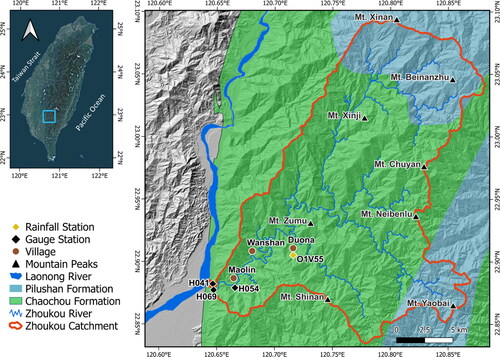
Our specific emphasis is on the Zhoukou River (Figure 1), which serves as a major tributary of the Laonong River. Based on information derived from the 20-m LiDAR DEM, the Zhoukou River Basin drains nearly 27% of the Laonung watershed. It covers an area of 375 km² and the trunk channel stretches for a total length of 32 km. The Zhoukou River Basin elevation ranges from 133 to 3290 meters and has an average slope of 36°. Its course predominantly over two major lithological formations, namely, the Pilushan Formation, which consists of phyllite, slate, and layers of quartzitic sandstone, and the Chaochou Formation, which includes slate, sandstone, argillite, and phyllite. The Zhoukou River Basin has been selected as our study site due to its active erosion, featuring ongoing and historical landslides as the primary mechanisms of erosion in the area. Over the past 31 years (1990–2020), annual rainfall in the Zhoukou River Basin ranged from 1706 mm to 5797 mm, averaging 3154.45 mm annually (data sourced from rainfall monitoring stations number 01P260, O1V55 maintained by WRA, Taiwan). The basin experiences a tropical to subtropical monsoon climate (Hsieh and Chyi 2010), with the majority of rainfall occurring from May to September due to typhoons that bring heavy rainfall in southern Taiwan (Wu and Kuo 1999).

Figure 1. Geologic map and geographic location of the study area: (top left) Orthoimage of Taiwan, blue box showing the location of the study area; (right) Map of Zhoukou River Basin, red polygon marks the catchment boundary. The Zhoukou River mainly drains over Pilushan and Chaochou formations, and it serves as a major tributary of the Laonong River. Associated lithological units over which the river flows are shown along with gauge (black diamond marker) and rainfall station (yellow diamond), and all the major mountain peaks in and around the Zhoukou River Basin are indicated. Multiple residential villages (brown dots) are also located downstream in the study area. 

The dynamic evolution of the Zhoukou basin, particularly in response to historical extreme rainfall events, is shown in Figure 2 through a series of satellite images for the period 1990 to 2020, sourced from Google Earth historical images. Additionally, we conducted bare land proportion analysis to show the basin’s dynamic nature over time (Figure 3). The basin is susceptible to frequent landslides and debris flows, triggered mainly by heavy rainfall associated with typhoons, resulting in the exposure of hill slopes as bare land devoid of vegetation cover (Chen et al. 2015). As a result, the majority of bare land areas are primarily a consequence of natural occurrences like landslides rather than being caused by human activities. Human development activities are very limited in the study area (Chang et al. 2015), minimizing factors such as deforestation, urbanization, and improper land management practices that could exacerbate erosion. Furthermore, human-occupied settlements constitute a very small fraction (less than 1%) downstream of the study area, as evidenced by the recent ESRI LULC (Land use/Land cover) 10-meter resolution map reinforcing that observed erosion is primarily driven by natural processes. Moreover, the Zhoukou River is well-equipped with hydrological gauge stations that record suspended sediment load (Figure 4, lower panel). This enables a comparison between erosion rates calculated from DoD and the erosion rate derived from suspended sediment loads in the river. By investigating erosion rates through this independent approach, we offer new volumetric change estimates at decadal-scale for understanding erosional and sediment transport processes in Taiwan’s active mountainous landscapes.

Figure 2. Google Earth historical images of the Zhoukou River Basin (1990–2020).  The different panels in the figure display a series of historical satellite images sourced from Google Earth, illustrating the evolution of the Zhoukou River Basin following extreme rainfall occurrences between 1990 and 2020. The red triangles shown in the middle timeline mark the timing of these extreme events.  Panels marked as a, b, c, and d (highlighted with blue dots on the timeline) depict the Zhoukou River Basin before and after the extreme events. It’s noteworthy that no extreme events were recorded between 2010 and 2020. Notably, during this latter decade, there appears to be a visible trend of vegetation recovery within the basin, indicating a potential rejuvenation of vegetation cover.

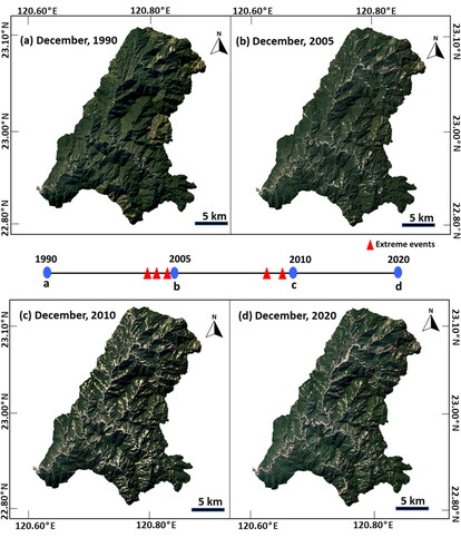
Figure 3. Bare land proportion of the Zhoukou River Basin after the extreme events. Bare land area was analyzed using Landsat imagery acquired from Landsat 5, Landsat 8, and the recently launched Landsat 9 satellites. Bare land area increased to 2.35 percent after the major extreme events in July 2004 and July 2005. The most extreme event in 2009, i.e. typhoon Morakot, increased the bare land proportion to 4.85 percent. After that, no significant extreme events have happened in the last decade. The bare land proportion as of the year 2020 was 3.38 percent, which indicated that vegetation cover had been restored considerably. However, the vegetation cover of the basin is still lower than pre-Morakot time, which suggests that vegetation recovery from the large-scale and deep-seated landslides can be difficult.

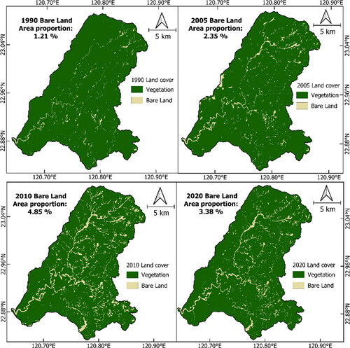
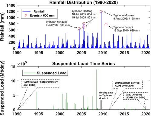
Figure 4. (a) The upper panel illustrates the daily rainfall data recorded by the Dona (01P260 & O1V55) rainfall monitoring station from 1990 to 2020, with major typhoon-induced rainfall events in the study area indicated. (b) The lower panel depicts the suspended load data time series of the Zhoukou basin compiled from three stations: 1730H041, 1730H054, and 1730H069. Suspended load data were sampled bi-weekly on average, amounting to a total of 643 data points for the period 1990–2020. The black dashed polygon indicates the time, resolution, and source of DEM used in the study area. 

3. Documented erosion rates in Taiwan

Erosion rates in Taiwan have garnered significant scientific attention due to its unique geological setting and intense rainfall events (Dadson et al. 2003; Willett et al. 2003). They have long been the subject of intriguing research, investigated across various temporal scales using established methodologies (Fuller et al. 2003; Siame et al. 2011). By examining erosion rates over different time spans, studies have aimed to gain insights into the complex interplay between natural forces like tectonics and climate in Taiwan (Dadson et al. 2003; Chen et al. 2020). For simplicity, we can classify the time scale of these studies into short-term (a few decades), intermediate-term (a few hundred to thousands of years), and long-term (several millions of years) and thereafter present a short summary of the available erosion rates at various timescales.

Short-term erosion rates (10⁰–10² yrs): Suspended load data from the gauge stations has been typically used to estimate catchment-scale, short-term erosion rates. Li (1976) estimated an average erosion rate of 5.5 mm/yr using suspended load data from gauge stations in the Central Range. Fuller et al. (2003) employed a combination of deterministic and stochastic hydrological modeling, estimating erosion rates between 2.2 and 8.3 mm/yr in the Eastern Central Range. Dadson et al. (2003) used 30 years of suspended load data from multiple hydrological stations across Taiwan and suggested a mean erosion rate of 5.2 mm/yr for the entire island (assuming a bedload proportion of 30%). Their decadal-scale erosion rate calculations revealed spatial variations with higher erosion rates in eastern central and southwest Taiwan, with a maximum value of 60 mm/yr in southwest Taiwan, near active thrust faults of the western foothill thrust belt. In contrast, lower values ranging from 1–4 mm/yr were observed in north and west Taiwan. Li et al. (2005) re-evaluated hydrological gauge station data for Kaoping River, yielding lower suspended load values than that of previous studies (Li 1976), highlighting potential bias in data collection, emphasizing the importance of large time series datasets to reduce uncertainty and account for temporal variations.

Intermediate-term erosion Rates (10³–10⁵ yrs): Studies based on in situ-produced cosmogenic ¹⁰Be in river-borne quartz minerals provide intermediate-term erosion rates over several hundreds to thousands of years of timescale. Siame et al. (2011) measured ¹⁰Be cosmogenic nuclide in quartz minerals from the Lanyang River in Northeast Taiwan, estimating an erosion rate of 2 ± 1 mm/yr. Derrieux et al. (2014) quantified denudation rates at the orogeny scale across the entire Taiwan island, ranging from 1–5 mm/yr, based on in-situ ¹⁰Be concentration. Fellin et al. (2017) derived erosion rates from cosmogenic nuclide concentration and detrital fission track ages in rivers of eastern Taiwan, revealing variations from less than 1 mm/yr in southern Taiwan to over 4 mm/yr in central Taiwan. Deng et al. (2020) used the ¹⁰Be(meteoric)/⁹Be system to derive denudation rates in the Zhoushui River Basin located in central Taiwan and found the rates to be between 1 and 8 mm/yr across different parts of the basin. In another study, Deng et al. (2021) examined denudation rates in the Liwu Basin in northeastern Taiwan and found the rates to be highly variable and range from ∼3 to >30 mm/yr.

Long-term erosion rates (>10⁶ yrs): Long-term erosion rates spanning millions of years timescales have been studied extensively in Taiwan using low-temperature thermochronometry. Liu (1982; Liu et al. 2000, 2001) determined a long-term erosion rate in the entire central range to be in the range of 2.5–4.6 mm/yr. Dadson et al. (2003) proposed long-term erosion rates ranging from 1 to 10 mm/yr for the entire island and 3–6 mm/yr for the Central Range using fission track data and a thermo-mechanical model. Willett et al. (2003) applied a similar methodology to the Eastern Central Range, determining long-term erosion rates in the range of 4–6 mm/yr. Fuller et al. (2006) and Simoes et al. (2007) incorporated data from low-temperature thermochronology and applied two-dimensional thermo-kinematic and thermo-mechanical models to re-evaluate long-term erosion rates, spanning from 2.3 mm/year to 3.2 mm/year.

4. Materials and methods

The DoD method used in the study, as the name suggests, involves the utilization of multi-temporal DEMs to estimate the cell-by-cell change in elevation between the DEMs. This approach provides insights into the volumetric change and erosion rate occurring between the two topographic surveys. However, a crucial challenge associated with employing the DoD method revolves around addressing the uncertainties inherent in the DEM datasets. One of the primary considerations in using the DoD method is ensuring that the desired elevation change signal surpasses the noise inherent in the datasets (Wheaton et al. 2010). The noise associated with DEM can be from multiple potential sources either during acquisition or during processing of the datasets, all of which get propagated into the DoD maps while using this method. Noise associated with the older elevation datasets, such as the photogrammetry-based DEM used in this study, may be unknown. Few studies have used DEM derived from similar technology (SAR Interferometry) to quantify decadal change in topography (Purinton and Bookhagen 2018). Using DEMs acquired from different techniques for detecting decadal change in topography can be challenging (Hsieh et al. 2016).

Given the geomorphological setting of Taiwan, having one of the highest erosion rates in the world provides us an excellent opportunity to use this method. By focusing on a decadal scale, we aim to capitalize on the accumulation of a substantial erosional signal, thereby enhancing the clarity and robustness of our findings. The decadal timescale provides ample time for the discernment of significant geomorphological changes, amplifying the clarity and depth of our erosion rate analysis. In situations where the magnitude of geomorphic change is substantial and surpasses the noise associated with the surveys or datasets, the DoD method indeed becomes a reliable tool. The high erosion rates in Taiwan provide a favorable environment for this method to excel. The distinctive nature of geomorphic changes in Taiwan ensures a favorable signal-to-noise ratio, thereby enhancing the accuracy of erosion rate calculations. Steps taken to derive accurate erosion rates using the DoD method are explained in the following sections and Figure 5.

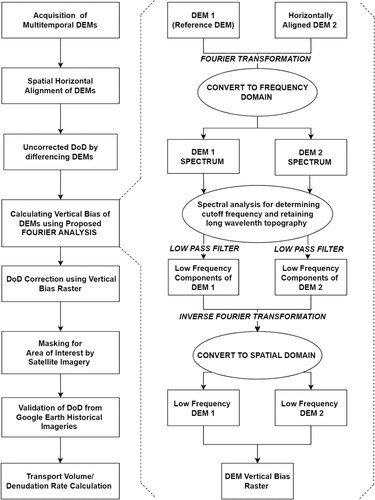
Figure 5. Workflow of the study illustrating the processing steps applied to various multitemporal DEMs (Digital Elevation Models). A novel approach utilizing Fourier transformation of DEMs has been implemented for vertical referencing, a crucial step in calculating denudation rates for the study area. The methodology involves using DEMs of Difference (DoD) to analyze the topographical changes over time.

4.1. DEM preparation, horizontal alignment, and uncorrected DoD calculation

For this study, we acquired three DEMs from various sources, as outlined in Table 1. All acquired DEMs were projected onto the same coordinate system (TWD97 system [EPSG:3826]). To delineate catchments, several steps were undertaken, including filling sinks in the terrain, determining the flow direction, and analyzing flow accumulation. Spatially alignment of DEMs was done in order to minimize the horizontal errors between the two DEMs so that we can only focus on elevation differences between the datasets. The recent LiDAR DEM was used as reference DEM for georeferencing, as it has the finest spatial resolution among all the datasets used. Control points were taken outside the catchment. Distinct features were used as control points to horizontally align the DEMs, such as road intersections and bridge intersections were available. After horizontal alignment of DEMs, uncorrected DoD were calculated by differencing the ALOS 3D DEM and TWPDEM respectively from LiDAR DEM. Further details of DEMs used in the study are mentioned below:

Table 1. DEM datasets used in the study.

Dataset	Data collection period	Native cell size(m)	Horizontal, vertical datums	Vertical accuracy	Creation method	Source
TWPDEM	1990	40	TWD67, TWVD79	1–4 m (Chen et al. 2005, 2006; Chan et al. 2007)	Aerial photogrammetry	Aerial survey office, Taiwan
ALOS 3D DEM	2006–2011	30	WGS84, EGM96	< 5 m (Tadono et al. 2016; JAXA 2015)	Satellite photogrammetry	Public, JAXA
LiDAR DEM	2020	20	TWD97, TWVD2001	< 1 m (MoI Taiwan)	Airborne LiDAR	Public, MoI Taiwan

1. TWPDEM (Aerial photogrammetry-based Taiwan DEM) – The most commonly used DEM in the past for the whole island was made by aerial photographs by aerial survey office in Taiwan with a horizontal resolution of 40m. The aerial photographs used for making DEM spans from the late 1980s to 1990. So, we used the latest year as the DEM production year. The vertical accuracy of TWPDEM is between 1–4 m depending on the terrain types, such as flat or mountainous areas (Chen et al. 2005).

2. ALOS 3D DEM – The ALOS World 3D DEM was first released in May 2016 with global coverage and is freely available in 30m horizontal resolution for public use. ALOS 3D DEM is produced based on its 5m commercial product, ‘World 3D Topographic Data’, which is considered to have the most vertical accuracy among all global DEM datasets (Uuemaa et al. 2020). The high precision of the ALOS 3D DEM dataset among all other global datasets has been attributed to its original 5m spatial resolution, which is then resampled to 30m resolution to create the ALOS 3D DEM dataset. It is a product of the optical sensor called PRISM (Panchromatic Remote-sensing Instrument for Stereo Mapping), which was equipped within the ALOS satellite and operated by the Japan Aerospace Exploration Agency (JAXA). For this study, we used the freely available 30m resolution DEM.

3. LiDAR DEM – This dataset was produced using an airborne LiDAR survey and is available in 20m horizontal resolution. This 20m LiDAR DEM possesses a vertical accuracy of a few decimeters and is the most accurate dataset among all DEMs used in this study. This DEM is maintained by Taiwan’s Ministry of the Interior (MoI) and is accessed from their open data repository (data.gov.tw).

4.2. DEM vertical referencing

In DoD analysis, achieving alignment between datasets is pivotal when comparing them for topographical change detection. However, discrepancies often arise due to multiple factors such as georeferencing inconsistencies, unknown coordinate system transformations, vertical datum variations, or distortions induced during instrument usage or DEM creation (Day and Muller, 1988). To address these discrepancies, several coregistration methods have been developed, each with its own set of strengths and limitations (Besl and McKay 1992; Nuth and Kääb 2011). The Nuth and Kääb (2011) approach primarily focuses on iterative translation and vertical shift estimations. It resolves discrepancies between DEMs by iteratively solving a cosine equation to determine the most likely offset direction and applying horizontal shifts accordingly. Another method, the tilt correction (Javernick et al. 2014; Girod et al. 2017), rectifies first-order polynomial errors between the reference and target DEMs. This method is particularly useful for correcting small rotations or nonlinear errors in datasets; it operates on a 2D plane and emphasizes vertical correction. The Iterative Closest Point (ICP) method, based on Besl and McKay (1992), corrects rigid transforms involving translation and rotation by iteratively aligning the data with the reference. In this context, our study introduces a novel method for vertical coregistration or referencing of DEMs to account for the vertical bias arising from different vertical datums of DEM datasets or any other systematic errors present in the DEM. We devised a novel approach, which uses Fourier transformation to change the spatial data, i.e. DEM, into the frequency domain. The frequency domain analysis of DEM helps in understanding the amplitude and periodicity of the topographical features. The underlying principle guiding our correction method is the distinct behavior of low-frequency and high-frequency components in DEMs. Low-frequency components capture long-wavelength variations within the terrain, typically associated with large-scale geological features and tectonic processes that evolve gradually over extended periods. The long wavelength topography of the DEMs, which was acquired within a 30-year temporal gap, ideally should remain the same. Any difference in the low-frequency component of these DEMs is representative of the vertical bias present in the DEM. High-frequency components, on the other hand, are susceptible to short-term changes, such as landslides, slope failures, and high-frequency noise. Our approach for vertical referencing of DEMs focuses on retaining low-frequency components and correcting vertical errors associated with these low-frequency components.

To achieve this, we harnessed the power of spectral analysis. This entailed converting the DEMs into the frequency domain using Fourier transformation. The 2D Discrete Fourier Transform (DFT) formula (followed from Perron et al. 2008; Booth et al. 2009; Purinton and Bookhagen 2017) used for this process involves the transformation of a square matrix of elevation values, denoted as z(x,y), with N_x×N_y measurements spaced evenly by Δx and Δy: (1) $$Z\left(k_x,k_y\right)=\sum _{m=0}^{N_x-1}{\sum }_{n=0}^{N_y-1}z(m\Delta x,n\Delta y)\mathrm{*}\mathrm{ }{e}^{-2\pi i\left(\mathit{\text{kx}}\mathrm{*}\frac{m}{N_x}+\mathit{\text{ky}}\mathrm{*}\frac{n}{N_y}\right)}$$(1)

Here, k_x​ and k_y​ represent wave numbers, while m and n serve as indices of z. This 2D DFT outputs an array showcasing the amplitudes of frequency components across both the x and y axes. The two orthogonal frequency components can be calculated from wavenumbers as: (2) $$f_x=\frac{k_x}{N_x\mathrm{\Delta }x},\hspace{1em}{f}_y=\frac{k_y}{N_y\mathrm{\Delta }y}$$(2)

Every element in Z(k_x,k_y) grid can be represented by a specific frequency called radial frequency which is $\sqrt{f_x^2+f_y^2}$ and a wavelength given by: (3) $$\lambda =\frac{1}{\sqrt{\left\{f_x^2+f_y^2\right\}}}$$(3)

From the 2D DFT array, the power spectrum is computed using the DFT periodogram: (4) $$P_{\mathit{\text{DFT}}}\left[(k_x,k_y)\right]=\frac{1}{N_x^2\cdot N_y^2}{\left|Z(k_x,k_y)\right|}^2$$(4)

The P_DFT array is a measure of the variance of z, denoted in units of amplitude squared (square meters). A one-dimensional power spectrum was generated by plotting this mean-squared amplitude against radial frequency (following methods from Perron et al. 2008; Booth et al. 2009; Purinton and Bookhagen 2017). Spectral power in topographical data usually diminishes with increasing frequency (Figure 6(b)). The data have been normalized by dividing it by the background spectrum (depicted by the black line in Figure 6(b), top) which highlights any variations or high-power peaks across the wavelengths (after Purinton and Bookhagen 2017). The power spectra of the DEMs provided critical insights into the distribution of topographic amplitudes across different wavelengths. We identified a wavelength threshold from the normalized power spectrum beyond which the short wavelength topography related to landslides, slope failures, and small-scale features were filtered out using a Gaussian low-pass filter. The low-pass filtered frequency components in the power spectra underwent inverse Fourier transformation to convert them back into the spatial domain. The low pass filtered DEMs now in spatial domain representing topographical features with wavelength ≥600 m lacks high-frequency disturbances and noise. These low passes filtered DEMs representing long wavelength topography ideally should remain same of all DEMs. The difference between these low-pass filtered DEMs are vertical bias present within the DEMs. LiDAR DEM is used as the reference DEM, given its higher vertical accuracy and RMSE of a few decimeters. So, the difference in low pass filtered DEM of TWPDEM and ALOS 3D DEM with low pass filtered DEM of LiDAR has been used to correct the respective original DoD.

Figure 6. Explanation of the proposed methods used for digital elevation model (DEM) filtering. Fourier transformations, spectral analyses, and low-pass filters are techniques used to remove vertical bias from the DEMs in order to vertically align the DEMs. This procedure separates the high-frequency components of DEM related to slope failures and landslides. Top: (a) DEM clip used for spectral analysis in the study area. (b) Non-normalized 1D power spectrum of topographic amplitudes across different wavelengths. Bottom: (c) Distribution of power across wavelengths (i.e. the inverse of radial frequencies) normalized by the background spectrum. The black line that represents the 99.99 percentile power envelope helps us in identifying the topographic wavelengths that have high power in the DEM. Fourier transformation methods have been adapted based on the works of Perron et al. (2008), Booth et al. (2009), and Purinton and Bookhagen (2017). (d) Gaussian low-pass filter that removes all wavelengths (λ) < 600 m and tapers to 700 m.

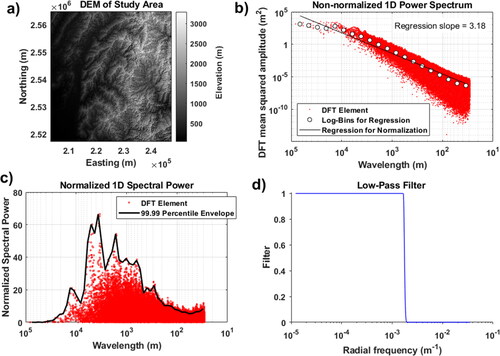
In our study, we set a wavelength threshold of ≥600 m for several reasons. One significant factor is the consideration of smaller-scale features. Wavelengths less than 600 m correspond to smaller-scale features and disturbances that are susceptible to short-term changes. By excluding these shorter wavelengths, we focused on retaining long wavelength components signifying long-term, large-scale variations in the terrain. Another important step in deciding wavelength threshold is spectral analysis of DEMs which indicates temporal consistency in long wavelength region. The examination of three temporal DEMs revealed a similar pattern of power envelope in the large wavelength region, extending up to approximately 600 m (refer to Figure 7). This indicates that topographic features with wavelengths greater than 600 m remained largely unchanged over the 30-year period. This temporal consistency of the power spectrum in the long wavelength region facilitated us to determine a threshold to separate the long and short wavelength topography in the study area. It is noteworthy that landslides in the study area typically exhibit wavelength scales of less than 500 m. Hence, by setting the threshold at 600 m, we effectively filtered out features associated with these short-wavelength disturbances.

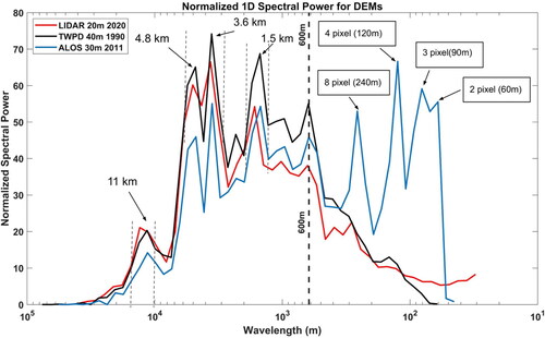
Figure 7. Normalized one-dimensional power spectra envelope for different DEMs used in the study. The 99.99 percentile power envelope is calculated from 20 logarithmically spaced bins to identify the dominant wavelength and isolate the low frequency (high wavelength) components of the DEMs. One-dimensional spectral analysis allowed us to identify the prominent topographic wavelengths present in the study area, which was a crucial step in separating high-frequency and low-frequency components.

4.3. Area of interest mask and denudation rate calculation

For quantifying change in topography from two DEMs, vegetation masks were created to identify changes in bare earth surface area and the regions that transitioned from vegetation to bare earth. This approach aimed to exclude areas that were consistently vegetated in both DEMs, effectively eliminating potential errors associated with DEMs containing vegetation height data. The presence of tree height within the DEM can lead to uncertainty in estimation of erosion rates when using the DoD approach, if the DEM doesn’t solely represent bare earth surfaces.

To pinpoint areas potentially experiencing active erosion, our focus is on recognizing alterations from vegetative to non-vegetative pixels between the two DEMs. The presence of non-vegetative pixels in both DEMs also signifies zones where active erosion might occur. To achieve this area of interest, ensuring focusing on pixels only indicative of potential erosion, creating a vegetation mask for the latter DEM is crucial. This approach allows us to isolate and analyze areas devoid of vegetation cover, enabling a precise estimation of regions experiencing potential active erosion within the defined study area. After analyzing our area of interest, it is appropriate to utilize a mask based on vegetative pixels for the latter year in the epoch, i.e. if we are detecting change between 1990 and 2020 DEM, a mask was generated for the 2020 DEM. This approach proved effective in preserving all vegetative pixels from the former period that underwent a transition to non-vegetative pixels in the latter period. Additionally, it retained all pixels that remained non-vegetative in both periods. By retaining the pixels showing potential areas of active erosion, we can successfully ignore the uncertainties associated from areas with dense vegetation. The mask layer for 2020 was created through the reclassification of land use and land cover data from the European Space Agency’s Sentinel-2 satellite imagery with a 10 m resolution.

The corrected DoD values were masked out for the defined area of interest. This was achieved by multiplying the mask layer prepared from 2020 DEM (with vegetation pixels assigned 0 and non-vegetative pixels assigned 1) with the corrected DoD layer. The resulting DoD values were further categorized into deposited areas (blue) and eroded (red), as shown in Figure 8. Sediment volume was calculated by multiplying the change in elevation with pixel area. Transported volume out of the system was determined by the difference between eroded and deposited volumes, represented by Equation (5)(5) $$V_t=V_e‐V_d=A({\sum }_{i=1}^N\Delta Z_i)$$(5) . (5) $$V_t=V_e‐V_d=A({\sum }_{i=1}^N\Delta Z_i)$$(5) where $V_t$ transported volume, $V_e$ is eroded volume (volume of all the negative pixels), $V_d$ is deposited volume (volume of all the positive pixels), $N$ is the total number of pixels with positive and negative elevation change, $A$ is the area of a single pixel, and Δ$Z_i$ is the elevation change of the ith pixel. Transported volume was then converted into denudation rate in mm/yr by the formula: (6) $$\frac{\mathit{\text{dz}}}{\mathit{\text{dt}}}=\frac{V_t}{A_b\Delta T}$$(6) where $V_t$ is Transported volume, $A_b$ is area of catchment and $\Delta T$ is the number of years between the two DEMs.

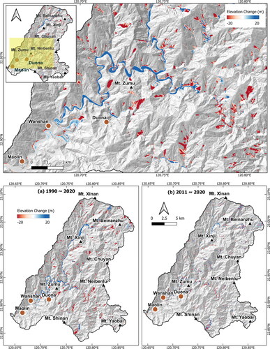
Figure 8. DEMs of Difference (DoD) Maps of the Zhoukou River Basin. Top panel shows the zoomed elevation difference map of area near the Maolin village within the Zhoukou River Basin for the period 1990–2020. This detailed view highlights sediment aggradation patterns in the main channel over the last three decades. The presence of multiple landslides in the catchment is discernible, showcasing signals of erosion in landslide scar areas and deposition in landslide toe areas. Bottom panel: (a) Illustration of the DoD map spanning 1990 to 2020, displaying the overall elevation changes and spatial distribution of sediment deposition (in blue, representing landslide toe and river deposition) and sediment erosion (in red, representing landslide scars and river bank erosion). (b) DoD map between the year 2011 and 2020, showing recent changes in elevation and sediment volume within the basin. Notably, the erosional and depositional signals appear less pronounced compared to the DoD map spanning 1990–2020, which is attributed to the absence of extreme events in recent times.

4.4. Calculation of denudation rates based on suspended sediment load

The Water Resources Agency (WRA) in Taiwan has set up more than 250 hydrometric stations. These stations are equipped to measure the water discharge (Q_W) on a daily basis, with more frequent measurements during typhoon or rainstorm events. To quantify the amount of suspended sediment in the rivers of Taiwan, the WRA collects water samples on an average of two to three times per month, with varying time intervals. To gather these samples, they utilize a DH-48 depth integrating suspended sediment sampler at each gauge station. The collected river water samples undergo a series of steps. First, they are filtered, and then they are subjected to a drying process followed by weighing. The concentration of suspended sediment in each sample is measured in parts per million (ppm). To calculate the suspended sediment discharge (Q_S), the corresponding water discharge (Q_W) is multiplied by a factor, sediment concentration (C). We estimated the erosion rates in the Zhoukou basin through two distinct methods. The first method involved the direct computation of erosion rates using mean suspended sediment load derived from suspended load records. The second method employed for determining erosion rates involved the application of rating curves derived from paired records of suspended sediment discharge and water discharge obtained from gauge stations.

4.4.1. Erosion rates based on the mean suspended sediment load

Utilizing data provided by the WRA, we accessed suspended sediment load records for the Zhoukou basin’s hydrometric stations. The mean suspended sediment discharge for the river was calculated by averaging recorded suspended sediment load values over varying observation periods. These periods ranged from a minimum of 123 observations (spanning 2006–2010) to a maximum of 266 observations (spanning 2011–2020). For these different monitoring periods, we converted the mean suspended load per day (mass/day) into sediment transport rates per year (volume/year), assuming an average rock density of 2.75 g/cm³. Normalizing the sediment transport rates by the basin area upstream from the respective gauging stations (as outlined in Table 2) facilitated the determination of catchment-averaged erosion rates. We analyzed erosion rates derived from the suspended load data obtained from three hydrometric stations located downstream near the mouth of the Zhoukou River (Figure 1).

Table 2. Estimation of denudation rate and sediment transport rate from mean sediment suspended load at three hydrological stations of the Zhoukou River Basin (H041, H054 and H069).

Gauge station number	Drainage area (km^2)	Years in record	Number of sediment observations	Mean water discharge (CMS)	Mean sediment concentration (ppm)	Mean suspended load (10^3 kg/day)	Sediment transport rate (Mm^3/yr)*	Denudation rate (mm/yr)^#	Sediment transport rate (Mm^3/yr)**	Denudation rate (mm/yr)^##
1730H041	375.08	10 (1994, 97–2005)	216	83.88	726.90	17598.87	2.33	6.24	3.34	8.92
1730H054	373.50	5 (2006–10)	123	57.87	947.065	24477.31	3.25	8.82	4.64	12.60
1730H069	374	10 (2011–20)	266	33.39	764.38	3236.46	0.43	1.15	0.61	1.64
1730H041 1730H054 1730H069	374	25 (1994–2020)	605	58.06	785.43	12900.05	1.71	4.58	2.45	6.54

*Sediment transport rate (Mm³/yr) = mean suspended load (10³ kg/day) × 365 (day/yr) ÷ rock density (2.75 × 10³ kg/m³) ÷ 10³ (suspended load only).

**Sediment transport rate (Mm³ /yr) = mean suspended load (10³ kg/day) × 365 (day/yr) ÷ rock density (2.75 × 10³ kg/m³) ÷ 10³ ÷ 0.7 (assuming that bedload proportion is 30%).

^#Denudation rate of basin based upon suspended load only.

^##Denudation rate of basin assuming the bedload proportion to be 30%.

4.4.2. Erosion rates based on the rating curve method

Determining the sediment discharge of a river becomes simpler when both Q_w (water discharge) and C (sediment concentration) are consistently measured at closely timed intervals. Nevertheless, due to the infrequent measurement of C, continuous records are often lacking. As a result, alternative approaches like sediment rating curves (Kao et al. 2005a) need to be employed. Based on the simple relationship between sediment concentration and water discharge, Fleming (1975) recommended a power law relationship: (7) $$C=a{Q}_w^b$$(7) where Q_W represents water discharge, typically measured in m³/s, while $a$ and $b$ are empirical constants. If the suspended concentration ($C$) is known from a gauge station, the suspended sediment discharge, $Q_s$ (in metric tons per day), can be calculated as: (8) $$Q_s=\mathit{\text{kC}}{Q}_w$$(8) where k is a conversion factor, reliant on the chosen units (0.0864 with the specified units). By using measurements of $C$ and applying Equations (7)(7) $$C=a{Q}_w^b$$(7) and (8)(8) $$Q_s=\mathit{\text{kC}}{Q}_w$$(8) , it becomes straightforward to quantify sediments as a function of water discharge: (9) $$Q_{\mathit{\text{Scalc}}}=A{Q}_w^b\text{with}A=\text{ka and B}=\text{b}+1$$(9)

We analyzed the erosion rate from the suspended load data from three hydrometric stations present downstream near the mouth of Zhoukou River. Using Equation (9)(9) $$Q_{\mathit{\text{Scalc}}}=A{Q}_w^b\text{with}A=\text{ka and B}=\text{b}+1$$(9) as proposed by Li et al. (2005), we calculated the parameters A and B, from the linear regression based on all available couples of data Q_W and Q_S. Thereafter, the same power law Equation (9)(9) $$Q_{\mathit{\text{Scalc}}}=A{Q}_w^b\text{with}A=\text{ka and B}=\text{b}+1$$(9) is applied to an entire set of daily water discharge data to evaluate the total suspended load per day. Suspended load discharge was then converted to transported volume by assuming a density of 2.75 g/cm^3. The transported volume was normalized by the drainage area upstream, and then the erosion rate was calculated. Comparing the erosion rates obtained through the mean sediment discharge method with those determined via the rating curve method allows for an evaluation of the efficacy and accuracy of these approaches.

5. Results

In this section, we present the results of utilizing spectral analysis techniques to improve the vertical referencing accuracy of DEMs and thereafter calculate sediment volumes and erosion rates through the corrected DoD map. Additionally, we present the erosion rates obtained from gauge stations based on mean suspended sediment discharge and rating curve method.

5.1. Spectral analysis for vertical referencing of DEMs

The power spectra of the DEM datasets help to identify wavelength threshold for preserving long wavelength topography. The low-frequency components were used to correct the vertical bias associated with different DEMs. The power spectra for different DEM also showed dominant long wavelength peaks at ∼ 11, 4.8, 3.6, and 1.5 km (Figure 7). We used a threshold of 600 m to remove all the wavelength associated with small-scale features, slope failures, and landslides. Reasons for choosing the threshold for retaining the long wavelength topography of DEMs have been discussed in Section 3.2 and Figure 7. In the power spectra analysis of the ALOS 3D DEM plotted against frequency, notable high-frequency peaks were observed at 2–8 pixels (60–240 m wavelength steps). Similar high-frequency spikes were previously identified in the power spectra of the 5 m AW3D5 DEM by Purinton and Bookhagen (2017). Given that the freely available 30 m ALOS DEM is derived from the downsampling of this AW3D5 DEM, it is plausible that these high-frequency and low-wavelength peaks represent the noise introduced during optical DEM generation through stereogrammetry, as suggested by Purinton and Bookhagen (2017). The low-frequency components identified in the spectral analysis of DEMs were retained through a low-pass Gaussian filter and utilized for generating long-wavelength topography via inverse Fourier transformation. We then derived the difference between these low-pass filtered DEMs. The difference serves as the vertical bias raster and is employed for vertical referencing of the DEMs in order to obtain a corrected DoD map.

5.2. Erosion rates derived from gauge stations based on the mean suspended sediment discharge

The erosion rates determined from two methods at gauge stations are presented in Tables 2 and 3. Erosion rates, derived from mean sediment discharge, range from 1.64 to 12.60 mm/yr. Notably, the erosion rate during the latest decade (2011–2020) is 1.64 mm/yr, representing the lowest value among all monitored periods. This lower rate can be attributed to a reduced occurrence of extreme events during this timeframe compared to other periods. Conversely, the highest erosion rate observed was 12.60 mm/yr for the 2006–2010 period. Overall, for the three-decade period, the mean erosion rate from suspended sediment (considering 30% bedload) is calculated to be 6.54 mm/yr. The variation of erosion rates across different time periods highlights the impact of extreme events on sediment discharge rate.

Table 3. Estimation of denudation rate and sediment transport rate from rating curve at three hydrological stations of the Zhoukou River Basin (H041, H054, and H069). Sediment rating curve (regression analysis diagrams) are in Figure 8.

Gauge station number	Drainage area (km^2)	Years in record	Number of daily discharge data (Qw)	Mean water discharge (CMS/day)	Mean suspended load (10^3 kg/day)	Sediment transport rate (Mm^3/yr)	Denudation rate (mm/yr)*
1730H041	375.08	16 (1990–2005)	4340	43.92	2384.80	0.45	1.2
1730H054	373.50	5 (2006–10)	1467	34.88	7568.45	1.44	3.85
1730H069	374	10 (2011–20)	2628	52.37	2575.83	0.49	1.31

*Denudation rate of basin based upon suspended load only (without bedload consideration).

5.3. Erosion rates derived from gauge stations based on the rating curve method

Erosion rates obtained from the rating curve method of different periods are lower than those estimated from the mean sediment discharge method. Erosion rates for the different periods from 1994–2020 range from 1.2 to 3.85 mm/yr from the rating curve method. In this calculation, bedload is not considered; if we consider the bedload to be 30% (Dadson et al. 2003), the erosion rate will be in the range of 1.71–5.5 mm/yr. However, when utilizing water discharge data to calculate the erosion rate, we found significant temporal gaps in the water flux record (see Figure 9, lower panel). Some gaps coincide with periods during and just after extreme events, indicating the absence of crucial high-water flow data. A single extreme event, such as a typhoon, can account for more than 75% of the total sediment flux from these small-mountainous rivers annually (Kao et al. 2005a; Kao and Milliman 2008). Consequently, the temporal gaps in water discharge records following these extreme events may introduce uncertainty and lead to underestimating the erosion rate.

Figure 9. Top panel: Regression analysis of suspended sediment discharge (Q_S) versus water discharge (Q_W) from three gauge stations in the Zhoukou River Basin. The station name and data period are indicated. Post-Morakot rating curve from the year 2011–2020 shows an increase in coefficient A and decrease in exponent b (refer to Equation (9)(9) $$Q_{\mathit{\text{Scalc}}}=A{Q}_w^b\text{with}A=\text{ka and B}=\text{b}+1$$(9) in the text), consistent with Huang and Montgomery’s findings (2013). Bottom panel: River discharge time series from 1990 to 2020. Grey blocks represent missing data in the daily water discharge record. Color in the time series of water discharge represents data from different gauge stations. Mean water discharge for respective stations in the given time periods are indicated. The location of the gauge station in the study area is shown in Figure 1. 

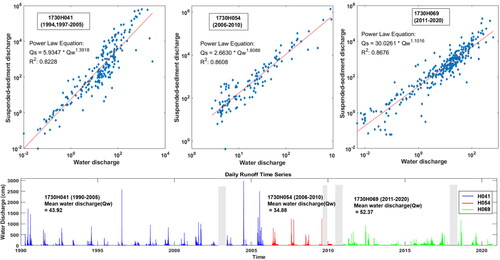
Fuller et al. (2003) suggested that erosion rates derived from rating curve methods become more reliable when the number of sediment observations exceeds 550 and the water discharge record length is greater than 6000. Erosion rates calculated from the mean sediment discharge method are more effective when rivers lack the aforementioned criteria. In our case, separate rating curves were computed for individual stations, each with a distinct monitoring period. However, all stations in the catchment have sediment observations fewer than 550. Given the limited number of sediment observations at each monitoring gauge station and the significant gaps in the water discharge record, we consider the erosion rate estimated from the mean suspended load to be closer to the true representation of the erosion rate in the basin, compared to the erosion rates estimated from the rating curve method.

5.4. Estimation of sediment volumes from the corrected DoD map

Using the corrected DoD map, the total erosional and depositional area has been calculated by counting the number of pixels showing negative and positive elevation differences and then multiplying the pixel counts with pixel area. Total erosional and depositional volume has been calculated by summation of the product of all the negative and positive pixels with the corresponding elevation difference. Total mobilized volume has been calculated by the difference between total erosional volume and depositional volume. Usually, in the fluvial environment, erosional volume is more than depositional volume in the system. The mobilized volume has been normalized by area and time gap to get the denudation rate per year. As shown in Figure 10, the total volume of mobilized sediments as per the corrected DoD map for the period 1990–2020 is 164.93 × 10⁶ m³. The total mobilized volume for the period 2011–2020 is 39.22 × 10⁶ m³. Compared to this, the uncorrected DoD gives a total mobilization volume of 458.59 × 10⁶ m³ for 1990–2020 and a volume of 281.02 × 10⁶ m³ for 2011–2020. The uncorrected DoD gives an overestimation of 178% and 616% respectively for the transported volume (Table 4). The erosional and depositional area for both the periods for the corrected and uncorrected DoD has been summarized in Table 4. As noted in Table 5, the uncorrected DoD tends to overestimate the erosional area and underestimate the depositional area, which is why overall overestimates the transported volume.

Figure 10. (Top) The histogram depicting the relationship between elevation differences and the corresponding affected area and volume across various periods. It shows the distribution of how much areas and volumes are impacted, corresponding to elevation differences. (Bottom) Total erosional, depositional, and mobilized volumes of different periods have been calculated and plotted along with the total erosional and depositional area.

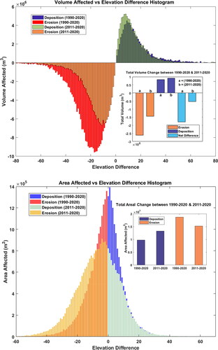
Table 4. Estimation of erosional, depositional and transported volumes from the corrected and uncorrected DoD.

Period	Method	Erosional volume (m³)	Depositional volume (m³)	Transported volume (m³)
1990–2020	Uncorrected DoD	577.41 × 10^6	118.82 × 10^6	458.59 × 10^6
	Corrected DoD	252.34 × 10^6	87.41 × 10^6	164.93 × 10^6
	Deviation before correction*	129 %	35.93 %	178 %
2011–2020	Uncorrected DoD	345.66 × 10^6	64.64 × 10^6	281.02 × 10^6
	Corrected DoD	136.62 × 10^6	97.40 × 10^6	39.22 × 10^6
	Deviation before correction*	153 %	−33.63 %	616 %

*Deviation before correction = ([Uncorrected DoD – Corrected DoD]/ Corrected DoD) *100 %.

Table 5. Estimation of erosional and depositional area from the corrected and uncorrected DoD.

Period	Method	Erosional area (m^2)	Depositional area (m^2)
1990–2020	Uncorrected DoD	20.29 × 10^6	8.23 × 10^6
	Corrected DoD	18.73 × 10^6	9.78 × 10^6
	Deviation before correction*	11 %	–15.84 %
2011–2020	Uncorrected DoD	20.12 × 10^6	8.39 × 10^6
	Corrected	15.24 × 10^6	13.28 × 10^6
	Deviation before correction*	32.02 %	−36.82 %

*Deviation before correction = ([Uncorrected DoD – Corrected DoD]/ Corrected DoD) *100 %.

The total erosional volume in the Zhoukou River Basin for the period 1990–2020 is 252.34 × 10⁶ m³, and the total depositional volume for the same period is 87.41 × 10⁶ m³, which signifies that not much of the sediment displaced from the hillslopes has been washed away from the catchment. A considerable amount of sediment is deposited as the newly formed alluvial fan, and a substantial amount is aggrading the main channel of the catchment (as seen in Figure 8, upper panel). Aggradation of up to 30 m was noticed in main channel of the Zhoukou River Basin. Using the uncorrected DoD technique to estimate the mobilized volume would lead to overestimation (Table 4). Applying the proposed method for DoD correction helps us to reduce the overestimation of volume by minimizing the vertical bias present within the DEMs.

6. Discussion

6.1. Accuracy assessment of corrected DoD after vertical referencing

In the context of coregistration approaches, a fundamental premise lies in the assumption that certain aspects of the depicted terrain remain unchanged between the reference and the DEM intended for alignment. This underlying stability within the terrain can be delineated by filtering out areas presumed to be volatile or dynamic. Consequently, the DEM slated for alignment undergoes transformation processes to conform as closely as possible to the stable regions depicted in the reference DEM. For our study, conducted in mountainous environments, identifying stable areas that remain unaffected by landslides, failed slopes, river channels, banks, and human-made changes is critical. Lack of precise ground control points can lead to uncertainty in using DoD for volume calculation in mountainous terrain. As previously discussed, the low-frequency components of the DEM serve as an indicator of stable terrain in a decadal timescale. In our investigation, we effectively extract this stable part of terrain by segregating features that are considered unstable. The Low pass filtered DEMs were used for DEM alignment process focusing on vertically correcting the dataset to ensure alignment with the reference DEM, thus leveraging the stability represented by the low-frequency terrain. This targeted correction methodology enables the alignment of DEMs by emphasizing stable terrain characteristics, thereby enhancing the accuracy of vertical referencing in our study’s context.

Hereby, we check the descriptive statistics of DoD with and without vertical referencing to compare the effectiveness of our correction method. Upon examining the descriptive statistics of the original and corrected DoD for the period 1990–2020, we can clearly observe significant improvements with original DoD having mean of −1.34, median of −0.82 and standard deviation of 25.57 and corrected DoD having mean of −0.01, median of −0.16 and standard Deviation of 13.63. Comparing the means, it’s evident that the original difference without referencing had a vertical bias that resulted in a mean value significantly different from zero. In contrast, the corrected difference data now exhibits a mean value closer to zero, indicating a substantial reduction in the bias. This means that the corrections have effectively mitigated the vertical bias, resulting in a more accurate representation of the elevation differences. The standard deviation has also significantly decreased from 25.57 to 13.63 signifying a reduction in the spread of difference values. This indicates that the corrections have successfully addressed the vertical bias and reduced variability in the difference data. The narrower spread suggests a more consistent and reliable representation of elevation differences.

A t-test was used to assess whether there is a significant difference in the means of corrected and uncorrected DoD. Since the two DoDs have unequal variance, we performed Welch’s t-test (Rogerson 2001). The t-test results provide robust evidence that the corrections made to the original difference DEMs have had a significant impact on the dataset. The null hypothesis (H0) of the t-test posited no significant difference between the means and distribution of values in the original and corrected DoD, with a significance level (α) set at 0.05. Our analysis yielded a remarkably low p-value of 0.0000, well below the significance level. Therefore, we confidently reject the null hypothesis. This clearly indicates that the corrected difference DEMs exhibit a statistically significant difference in means compared to the original data. The statistical significance confirms that the corrections have effectively eliminated the vertical bias and improved the accuracy of the dataset.

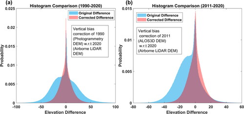
We also performed a comparison of histograms of the original and corrected DoD to check the improvement done by our correction method. Figure 11 depicts the histogram comparison showcasing the distribution of elevation difference values before and after the vertical referencing. The left histogram represents the original difference data, characterized by biases and irregularities. In contrast, the right histogram illustrates the distribution of elevation differences after applying corrections. The visual comparison highlights the substantial improvement in data quality, as the corrected histogram shows a more balanced distribution with reduced bias-related characteristics. The corrections have effectively addressed the vertical bias, resulting in a more accurate representation of elevation differences during the two time periods.

Figure 11. Histogram comparison of original and corrected DoD for the periods (a) 1990–2020 and (b) 2011–2020. The histograms illustrate the distribution of elevation differences before and after applying corrections for vertical referencing. The vertical referencing of the 1990 photogrammetry DEM (TWPDEM) and 2011 ALOS 3D DEM has been done with respect to the reference airborne LiDAR DEM. The corrections have successfully addressed the vertical bias and reduced variability in the elevation difference data. The shift towards a narrower distribution and a more centralized peak in the corrected histogram signifies a reduction in variability or bias. This narrower spread feature in the corrected DoD histogram indicates a consistent and reliable representation of elevation differences, reflecting a significant improvement achieved after applying vertical referencing corrections.

6.2. Erosion rates derived from corrected DoD versus other traditional approaches

We translated the exported volume out of the catchment for two different periods into denudation rate by normalizing it with respect to area and number of years according to Equation (6)(6) $$\frac{\mathit{\text{dz}}}{\mathit{\text{dt}}}=\frac{V_t}{A_b\Delta T}$$(6) . Our independent approach, based on the calculation of corrected DoD derived denudation rates on a catchment scale, yields values within the range of 10.46–14.19 mm/yr. This range can be considered a representation of erosion rates over shorter time durations and is indicative of the landscape response to extreme events occurring within that timescale.

The determined erosion rate in our study area encompasses the effects of short-term, high-frequency erosional events, such as extreme weather events (e.g. typhoons), human activities, and other transient factors. It effectively captures the rapid fluctuations in erosion rates that are characteristic of short-term dynamics. Therefore, our approach provides a comprehensive view of the erosional processes occurring within the decadal timescale. Furthermore, it is crucial to recognize that catchment-scale erosion rates are inherently influenced by various factors, including lithology, regional extreme events, and natural variability in different mountain catchments. As demonstrated by Dadson et al. (2003), who reported a regional erosion rate of up to 60 mm/yr in a catchment near an active fault of the western thrust fault in southwest Taiwan based on suspended load data, the variability in erosion rates is substantial across different regions. Additionally, Chen et al. (2015) conducted a comprehensive study on the Kaoping River Basin, of which the Zhoukou River is a tributary. Their findings, covering the study period from 2001 to 2009 and focusing on the impact of typhoon Morakot, revealed an average landslide erosion rate of 24.06 ± 1.54 mm/yr. This underscores the point that regional erosion rates can exhibit significant variability from catchment to catchment.

On the other hand, as discussed in Section 2, previous studies show that erosion rates can vary significantly for different timescales, including intermediate-term and long-term. This variation is attributed to several factors. Short-term erosion rates, which cover a few decades, are influenced by recent changes in erosion patterns and high-frequency events. On the other hand, other intermediated and long-term erosion, extending from thousands to over millions of years, reflects the cumulative impact of geological, tectonic, and climatic processes over deep geological time, resulting in significantly lower erosion rates but they tend to average out the immediate responses of the landscape to processes like heavy rainfall and typhoons.

One of the key advantages of our DoD method is its independence from traditional gauge station measurements. Denudation rates estimated from mean suspended load data from the gauge station are 6.54 mm/yr. and 1.64 mm/yr. Gauge station data collection methods can be subject to potential biases in data collection and missing data due to circumstances beyond human control, such as equipment breaking or malfunctioning during extreme events. As mentioned earlier, extreme events associated with the mountain river basins (Kao et al. 2005a; Kao and Milliman 2008) can significantly contribute to sediment output. Gauge stations have missing data (Figure 4, lower panel) corresponding to Typhoon Morakot, one of the most extreme events in Taiwan within the last 30 years, that can profoundly impact sediment dynamics. So, the omission of data from such events has the potential to lead to a substantial underestimation of erosion rates. Discrepancies have also been reported in the data recorded by the WRA at gauge stations from eastern Taiwan during low flow periods (Kao et al. 2005b). In their study, the authors question the sensitivity of measurements in the WRA record based on their field sampling from April 4 to May 5, 2003, which was conducted during a very dry period. These issues emphasize the challenges in the data collection methodologies of gauge stations. Erosion rate estimation from gauge stations relies solely on suspended load data while necessitating additional estimations for bed load data. In contrast, our DoD approach operates independently of gauge station data. By directly measuring erosion rates from the difference in elevation models, it provides a more direct and spatially comprehensive assessment of landscape changes at decadal time scale.

Furthermore, our approach leverages the global Digital Elevation Model derived from satellite data, which is freely available and underutilized. The use of Global and regional DEMs can give extensive coverage. This data availability enhances the appeal of our approach as an alternative for insights at the decadal-scale. It not only broadens the scope of data sources but also contributes to the accessibility of erosion rate assessments on a larger scale. As compared to the traditional intermediate and long-term erosion rate techniques such as cosmogenic nuclide analysis, zircon fission track analysis (ZFT), and apatite fission track analysis (AFT), which focuses on analyzing samples from specific locations or points within a geological or geomorphological setting, the DoD approach can provide comprehensive coverage of a larger area making it suitable for studying erosion rates on a regional or even global scale, capturing broader patterns and changes in the landscape. DoD can offer high spatial resolution based on the DEMs used, enabling the detection of fine-scale topographic changes critical for understanding localized erosion and deposition patterns. DoD approach is cost-effective, as it reduces the need for expensive fieldwork and specialized laboratory analyses common to other techniques, making it more accessible to a broader scientific community interested in large-scale landscape evolution studies.

6.3. Estimation of sediment export rates in different decades

Three DEMs from different decades, namely TWPDEM (1990), ALOS 3D DEM (2011), and LiDAR DEM (2020), were utilized to estimate sediment export rates for the first time in this study using the DoD technique with a newly developed method for vertical referencing of DEMs. Following necessary DoD corrections aimed at eliminating vertical biases associated with the DEMs, denudation rates for both the recent decade and former decades were determined. The denudation rate for the entire period from 1990 to 2020 is computed to be 14.19 mm/yr, while the denudation rate for the recent decade (2011–2020) is determined to be 10.46 mm/yr. The DoD maps generated for these two distinct periods effectively capture the signal of erosional events occurring within their respective time periods (Figure 8, lower panel). The erosion rate for the latter decade is found to be lower than that of the previous two decades. This trend is consistent with the mean erosion rate derived from limited available data at gauge stations, indicating a lower erosion rate of 1.64 mm/yr in the last decade and a relatively higher erosion rate of 6.54 mm/yr from 1990 to 2020.

The newly obtained erosion rates derived from the independent method of DoD at a decadal-scale can now complement erosion rates derived from other methods spanning longer timescales. This integration allows us to evaluate better and understand the landscape evolution of catchments in the active mountain belt of Taiwan. Erosion rates derived from gauge stations over decadal scales often underestimate short-term erosion rates. This limitation arises because, during extreme events, the monitoring stations may lack records due to the absence of sampling, instrument malfunction, or even destruction by high water discharge or debris flow. As a result, relying solely on decadal-scale data from the gauge stations might lead to an incomplete understanding of erosion dynamics, particularly in places like Taiwan, where rapid and intense erosional events are common. So, utilizing new erosion rates from our DoD at decadal-scale will give insights into the variability of erosion rates, especially during the extreme events that significantly impact the landscape. The better understanding of the variability of erosion rates is crucial for planning infrastructure projects, such as tunnels, bridges, and other civil developments.

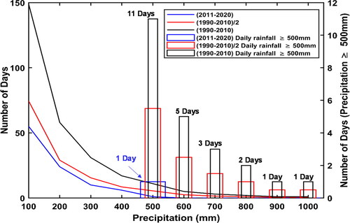
Our study shows that the decrease in annual sediment export rates during the most recent decade (2011–2020) compared to the preceding two decades (1990–2010) is attributed primarily to a reduction in extreme rainfall events. Figure 12 describes the frequency of days recording different precipitation for different decades. The black line and black bar represent data from the previous two decades, while the red line and red bar represent the same data normalized. The blue line and blue bar represent data from the recent decade (2011–2020). Our findings reveal a stark contrast between the recent decade (2011–2020) and the two preceding decades (1990–2010). A clear trend of higher number of days registering precipitation levels can be observed for the previous two decades in comparison to the recent decade. Throughout the recent decade, a mere single day registered daily rainfall exceeding 500 mm, a notable deviation from the average of 5.5 such events per decade in the previous two decades. Importantly, our records indicate a conspicuous absence of any daily rainfall surpassing 600 mm during 2011–2020, while the period of 1990–2010 documented five instances exceeding this threshold. This disparity in extreme rainfall occurrences notably corresponds to the reduced erosion rates observed in the recent decade. Chen et al. (2015) also highlighted that extreme-intensive rainfall events, particularly those with a maximum 24-h precipitation exceeding 600 mm, exert a significantly greater impact on hillslope mass wasting and contribute substantially to the total landslide erosion rate in the Kaoping River Basin. Our investigation aligns with the observations made by Chen et al. (2015), emphasizing the pivotal role of extreme rainfall events in influencing erosion rates. Several other significant studies, such as those by Galewsky et al. (2006), Chen et al. (2020), and Ruetenik et al. (2020), have highlighted the importance of the frequency of extreme events in delineating geomorphological changes in Taiwan. Kao and Milliman (2008) conducted a comprehensive analysis of sediment discharge data from 16 Taiwanese rivers, concluding that the majority of sediment flux discharge results from typhoon-generated floods. These studies indicate the significant role of these episodic events in sediment erosion and delivery from small mountainous rivers in Taiwan. Our findings, as illustrated in Figure 12, highlight the reason for variations in erosion rates during different periods. The rainfall statistics data show the fluctuation in the number of extreme events in each respective period, emphasizing the significant contribution of extreme events to erosion rates.

Figure 12. Frequency of days recording various levels of precipitation across different decades. Notice that there is no single daily precipitation event greater than 600mm in the period of 2011–2020.  This can be an explanation for the lower average erosion rate in the last decade compared to previous decades. The clear trend of no extreme precipitation events exceeding this threshold during the most recent decade is a crucial factor in understanding the reduced erosion rates within this timeframe.

6.4. Limitations and uncertainties of derived denudation rates

In evaluating denudation rates, it is crucial to recognize the potential uncertainties influenced by various factors. The elevation data in the initial DEM may not accurately represent the bare earth elevation during that period because of tree height bias. Therefore, the calculation of DoD has the potential to overstate the actual erosion rate, considering the presence of vegetation in the initial DEM. Also, the TWPDEM and ALOS 3D DEM were generated based on number of optical scenes spanning a few years. In this study, the most recent year of optical imagery utilized in the generation of these DEMs was designated as the reference year of the respective DEMs, using which in DoD analysis will essentially represent the upper limit for erosion rate estimates. Due to the varying resolutions of DEMs, we prioritized the precision and detail offered by the LiDAR 2020 DEM, which represents the highest resolution dataset available. In order to ensure consistency and comparability across datasets, lower-resolution DEMs were resampled to a 20-meter resolution prior to differencing. While this resampling process may introduce some interpolation artifacts or noise, our primary objective remains to accurately detect subtle changes in elevation post extreme events, capturing depositional and erosional dynamics to the fullest extent possible with available data. It is also essential to acknowledge the presence of high-frequency noise within the ALOS-derived DEM, introducing potential uncertainties in the erosion rate assessments. Despite the inherent noise in the optical DEMs, which may contribute to additional uncertainties, it is noteworthy that the observed patterns and localized hotspots of erosion and deposition remained discernible while using the ALOS 3D DEM for DoD analysis. This resilience in pattern recognition underscores the robustness of the optical DEMs in capturing the broader changes in landscape evolution, even in the presence of noise. While there may be a possibility of anthropogenic-related uncertainty, it’s important to note that human-occupied settlements constitute a very small fraction, less than 1% of the study area. Furthermore, human development activities are also very limited within the study area. Thus, the associated uncertainty from these activities is considered minimal in our case. Another limitation of the study may arise from the utilization of satellite images and global/regional DEMs, where the image resolution may not be sufficient to accurately classify the phenomena depicted in the DoD map. To better estimate various phenomena such as landslides, debris flows, channel aggradation, etc., contributing to the DoD map, further works could benefit from employing high-resolution local imagery.

We chose not to employ thresholding on the DoDs to calculate the total transported volume, as it could potentially obscure true erosion or deposition signals, as highlighted by Anderson (2019). To assess potential uncertainties present in the DoD dataset, significant works have been done using stable grounds present within the study area with no true elevation change (Anderson 2019; Schwat et al. 2023). However, our study area lacks spatially large and relevant stable areas, which makes it challenging to adopt this approach. Our method of vertical referencing in the frequency domain can alternatively be used in the absence of spatially relevant stable areas, which can mitigate potential systematic errors and vertical biases in the dataset. Future studies can benefit from this approach to minimize such errors in datasets lacking uniformly distributed stable points within the study area.

7. Conclusion

In this study, we employed three DEMs from different sources and techniques to estimate the mobilized volume from the Zhoukou River Basin in southwestern Taiwan. We utilized the ‘DEMs of Difference’ method, independent from traditional approaches, to estimate denudation rates at the mountain river basin scale. Our novel approach, incorporating Fourier analysis, effectively mitigated vertical bias in DEMs, making them suitable for the DoD method. By identifying low-frequency components representing stable topography, we preprocessed DEMs, enabling the estimation of topographic changes. The derived erosion rate presents an independent and efficient approach, distinct from traditional methods. Denudation rates over the span of three decades (1990–2020) were measured within the range of 10.46 to 14.19 mm/yr. By using underutilized global satellite-derived DEMs and regional DEMs, the DoD method offers a rapid means of extracting meaningful erosional signals. Despite limitations associated with DEM data, meaningful erosion rate estimations are achieved where the time lapse between DEMs and the magnitude of topographic change outweighs noise, particularly evident in dynamic landscapes like Taiwan. Comparisons with traditional erosion rate estimation methods reveal the value of DoD-derived erosion rates as an alternative to gauge station-derived rates, mitigating biases and offering insights into immediate landscape responses to natural phenomena and human activities.

Through the utilization of the DoD method, we quantified and revealed patterns of erosion (such as landslides and bank erosion), deposition (such as aggradation in the main river channel downstream), and net volumetric changes or sediment transport. These findings are necessary and helpful for comprehending the shaping of landscapes in mountainous river basins. The newly quantified decadal denudation rates can be useful for understanding how climatic conditions, such as heavy rainfall and typhoons, escalate erosion processes, capturing the immediate response of landscapes to these extreme events over short time periods. Variation in sediment export from the Zhoukou River Basin demonstrates the impact of small mountainous rivers on biogeochemical element transfer to the ocean. This quantification of mobilized volume also aids in civil planning and construction, allowing for proactive measures based on decadal-scale volume mobilization trends at the catchment scale. Such information of denudation rates can enhance the accuracy of models simulating the intricate interplay between tectonic uplift, erosion, and landscape evolution. By assessing erosion rates at the catchment scale, our research can complement erosion rates derived from other traditional approaches at different timescales, improving our understanding of the temporal patterns of landscape evolution of mountainous river basins in Taiwan, with potential applicability to similar regions worldwide.

Acknowledgments

We are grateful for the support and resources provided by Taiwan International Graduate Program (TIGP), Department of Earth Sciences, National Central University, and the Institute of Earth Sciences, Academia Sinica, Taiwan. We are also thankful to JAXA, Japan, the Aerial Survey Office and the Ministry of the Interior, Taiwan for providing the open-source datasets used in the study. We are thankful to the anonymous reviewers for their valuable and constructive comments which significantly improved the quality of the manuscript.

Data availability statement

The Alos World 3D DEM is openly available and can be found at https://www.eorc.jaxa.jp/ALOS/en/dataset/aw3d30/aw3d30_e.htm. Hydrological data from gauge stations can be obtained from the Water Resources Agency of Taiwan. Photogrammetry DEM data is obtained from the Aerial Survey Office of Taiwan, while 20 m DEM data is acquired from the open data repository (data.gov.tw) maintained by the Ministry of the Interior, Taiwan.

Disclosure statement

No potential conflict of interest was reported by the author(s).

Correction Statement

This article has been corrected with minor changes. These changes do not impact the academic content of the article.

Additional information

Funding

This work was supported by National Science and Technology Council, Taiwan under grant [NSTC 112-2119-M-259-004] and [NSTC 112-2116-M-001-027].

References

- Allen PA. 1997. Earth surface processes. Malden (MA): John Wiley & Sons.
- Anderson SW. 2019. Uncertainty in quantitative analyses of topographic change: error propagation and the role of thresholding. Earth Surf Processes Landf. 44(5):1015–1033. doi: 10.1002/esp.4551.
- Arrell K, Wise S, Wood J, Donoghue D. 2008. Spectral filtering as a method of visualising and removing striped artefacts in digital elevation data. Earth Surf Processes Landf. 33(6):943–961. doi: 10.1002/esp.1597.
- Besl PJ, McKay ND. 1992. A method for registration of 3-D shapes. IEEE Trans Pattern Anal Mach Intell. 14(2):239–256. doi: 10.1109/34.121791.
- Bishop P. 2007. Long‐term landscape evolution: linking tectonics and surface processes. Earth Surf Processes Landf. 32(3):329–365. doi: 10.1002/esp.1493.
- Booth AM, Roering JJ, Perron JT. 2009. Automated landslide mapping using spectral analysis and high-resolution topographic data: Puget Sound lowlands, Washington, and Portland Hills, Oregon. Geomorphology. 109(3–4):132–147. doi: 10.1016/j.geomorph.2009.02.027.
- Bull WB. 1984. Tectonic geomorphology. J Geol Educ. 32(5):310–324. doi: 10.5408/0022-1368-32.5.310.
- Chan YC, Chen YG, Shih TY, Huang C. 2007. Characterizing the Hsincheng active fault in northern Taiwan using airborne LiDAR data: detailed geomorphic features and their structural implications. J Asian Earth Sci. 31(3):303–316. doi: 10.1016/j.jseaes.2006.07.029.
- Chang CH, Harrison JF, Huang YC. 2015. Modeling typhoon-induced alterations on river sediment transport and turbidity based on dynamic landslide inventories: Gaoping River Basin, Taiwan. Water. 7(12):6910–6930. doi: 10.3390/w7126666.
- Chen CY, Willett SD, West AJ, Dadson S, Hovius N, Christl M, Shyu JBH. 2020. The impact of storm-triggered landslides on sediment dynamics and catchment-wide denudation rates in the southern Central Range of Taiwan following the extreme rainfall event of Typhoon Morakot. Earth Surf Processes Landf. 45(3):548–564. doi: 10.1002/esp.4753.
- Chen RF, Chan YC, Angelier J, Hu JC, Huang C, Chang KJ, Shih TY. 2005. Large earthquake-triggered landslides and mountain belt erosion: the Tsaoling case, Taiwan. Comptes Rendus. Géoscience. 337(13):1164–1172. doi: 10.1016/j.crte.2005.04.017.
- Chen RF, Chang KJ, Angelier J, Chan YC, Deffontaines B, Lee CT, Lin ML. 2006. Topographical changes revealed by high-resolution airborne LiDAR data: the 1999 Tsaoling landslide induced by the Chi-Chi earthquake. Eng Geol. 88(3–4):160–172. doi: 10.1016/j.enggeo.2006.09.008.
- Chen YC, Chang KT, Chiu YJ, Lau SM, Lee HY. 2013. Quantifying rainfall controls on catchment‐scale landslide erosion in Taiwan. Earth Surf Process Landf. 38(4):372–382. doi: 10.1002/esp.3284.
- Chen YC, Chang KT, Lee HY, Chiang SH. 2015. Average landslide erosion rate at the watershed scale in southern Taiwan estimated from magnitude and frequency of rainfall. Geomorphology. 228:756–764. doi: 10.1016/j.geomorph.2014.07.022.
- Dadson SJ, Hovius N, Chen H, Dade WB, Hsieh ML, Willett SD, Hu JC, Horng MJ, Chen MC, Stark CP, et al. 2003. Links between erosion, runoff variability and seismicity in the Taiwan orogen. Nature. 426(6967):648–651. doi: 10.1038/nature02150.
- Davies TR, Korup O. 2010. Sediment cascades in active landscapes. In: Sediment cascades: an integrated approach. Chichester (UK): John Wiley and Sons. p. 89–115.
- Day T, Muller J-PAL. 1988. Quality assessment of digital elevation models produced by automatic stereomatchers from SP OT image pairs. Photogrammetr. Record. 12(72):797–808.
- Deng K, Wittmann H, Yang S, von Blanckenburg F. 2021. The upper limit of denudation rate measurement from cosmogenic 10Be(Meteoric)/9Be ratios in Taiwan. JGR Earth Surf. 126(10):e2021JF006221. doi: 10.1029/2021JF006221.
- Deng K, Yang S, von Blanckenburg F, Wittmann H. 2020. Denudation rate changes along a fast-eroding mountainous river with slate headwaters in Taiwan from 10Be (Meteoric)/9Be ratios. JGR Earth Surf. 125(2):e2019JF005251. doi: 10.1029/2019JF005251.
- Derrieux F, Siame LL, Bourlès DL, Chen RF, Braucher R, Léanni L, Lee JC, Chu HT, Byrne TB. 2014. How fast is the denudation of the Taiwan mountain belt? Perspectives from in situ cosmogenic 10Be. J Asian Earth Sci. 88:230–245. doi: 10.1016/j.jseaes.2014.03.012.
- Fellin MG, Chen CY, Willett SD, Christl M, Chen YG. 2017. Erosion rates across space and timescales from a multi-proxy study of rivers of eastern Taiwan. Global Planet Change. 157:174–193.
- Fleming G. 1975. Computer simulation techniques in hydrology. New York (N.Y.): Elsevier.
- Fuller CW, Willett SD, Hovius N, Slingerland R. 2003. Erosion rates for Taiwan Mountain Basins: new determinations from suspended sediment records and a stochastic model of their temporal variation. J Geol. 111(1):71–87. doi: 10.1086/344665.
- Fuller C, Willett S, Fisher D, Lu CY. 2006. A thermomechanical wedge model of Taiwan constrained by fission-track thermochronometry. Tectonophysics. 425(1–4):1–24.
- Galewsky J, Stark CP, Dadson S, Wu CC, Sobel AH, Horng MJ. 2006. Tropical cyclone triggering of sediment discharge in Taiwan. J Geophys Res. 111(F3):F03014. doi: 10.1029/2005JF000428.
- Girod L, Nuth C, Kääb A, McNabb R, Galland O. 2017. MMASTER: improved ASTER DEMs for elevation change monitoring. Remote Sens. 9(7):704. doi: 10.3390/rs9070704.
- Hsieh ML, Capart H. 2013. Late Holocene episodic river aggradation along the Lao-nong River (southwestern Taiwan): an application to the Tseng-wen Reservoir Transbasin Diversion Project. Eng Geol. 159:83–97. doi: 10.1016/j.enggeo.2013.03.019.
- Hsieh ML, Chyi SJ. 2010. Late quaternary mass-wasting records and formation of fan terraces in the Chen-yeo-lan and Lao-nung catchments, central-southern Taiwan. Quat Sci Rev. 29(11–12):1399–1418. doi: 10.1016/j.quascirev.2009.10.002.
- Hsieh YC, Chan YC, Hu JC. 2016. Digital elevation model differencing and error estimation from multiple sources: a case study from the Meiyuan Shan landslide in Taiwan. Remote Sens. 8(3):199. doi: 10.3390/rs8030199.
- Huang MYF, Montgomery DR. 2012. Fluvial response to rapid episodic erosion by earthquake and typhoons, Tachia River, central Taiwan. Geomorphology. 175–176:126–138. doi: 10.1016/j.geomorph.2012.07.004.
- Javernick L, Brasington J, Caruso B. 2014. Modeling the topography of shallow braided rivers using structure-from-motion photogrammetry. Geomorphology. 213:166–182. doi: 10.1016/j.geomorph.2014.01.006.
- JAXA. 2015. ALOS Global Digital Surface Model “ALOS World 3D – 30m (AW3D30)”, Japan Aerospace Exploration Agency. https://www.eorc.jaxa.jp/ALOS/en/dataset/aw3d30/aw3d30_e.htm.
- Kao SJ, Chan SC, Kuo CH, Liu KK. 2005b. Transport-dominated sediment loading in Taiwanese Rivers: a case study from the Ma-an stream. J Geol. 113(2):217–225. doi: 10.1086/427670.
- Kao SJ, Lee TY, Milliman JD. 2005a. Calculating highly fluctuated suspended sediment fluxes from mountainous rivers in Taiwan. Terrestrial Atmos Ocean Sci. 16(3):653.
- Kao SJ, Milliman JD. 2008. Water and sediment discharge from small mountainous rivers, Taiwan: the roles of lithology, episodic events, and human activities. J Geol. 116(5):431–448. doi: 10.1086/590921.
- Kirby E, Whipple KX. 2012. Expression of active tectonics in erosional landscapes. J Struct Geol. 44:54–75. doi: 10.1016/j.jsg.2012.07.009.
- Li FC, Angelier J, Chen RF, Hsieh HM, Deffontaines B, Luo CR, Wu TT, Lin MC. 2005. Estimation de l’érosion actuelle à partir du transport de sédiments par les rivières: une étude de cas à Taiwan. Comptes Rendus – Geosci. 337(13):1131–1139. doi: 10.1016/j.crte.2005.05.001.
- Li YH. 1976. Denudation of Taiwan island since the Pliocene epoch. Geol. 4(2):105–107. doi: 10.1130/0091-7613(1976)4<105:DOTIST>2.0.CO;2.
- Liu JP, Liu CS, Xu KH, Milliman JD, Chiu JK, Kao SJ, Lin SW. 2008. Flux and fate of small mountainous rivers derived sediments into the Taiwan Strait. Mar Geol. 256(1–4):65–76. doi: 10.1016/j.margeo.2008.09.007.
- Liu TK, Chen YG, Chen WS, Jiang SH. 2000. Rates of cooling and denudation of the Early Penglai Orogeny, Taiwan, as assessed by fission-track constraints. Tectonophysics. 320(1):69–82. doi: 10.1016/S0040-1951(00)00028-7.
- Liu TK, Hsieh S, Chen YG, Chen WS. 2001. Thermo-kinematic evolution of the Taiwan oblique-collision mountain belt as revealed by zircon fission track dating. Earth Planet Sci Lett. 186(1):45–56. doi: 10.1016/S0012-821X(01)00232-1.
- Liu TK. 1982. Tectonic implication of fission track ages from the Central Range, Taiwan. Proc Geol Soc China. 25:22–37.
- Malavieille J. 2010. Impact of erosion, sedimentation, and structural heritage on the structure and kinematics of orogenic wedges: analog models and case studies. GSAT. 20(1):4–10. doi: 10.1130/GSATG48A.1.
- Marks RJ. 2009. Handbook of Fourier analysis & its applications. New York (NY): Oxford University Press.
- Milliman and Farnsworth. 2011. River discharge to the coastal ocean: a global synthesis. Cambridge (UK): Cambridge University Press; p. 384.
- Nuth C, Kääb A. 2011. Co-registration and bias corrections of satellite elevation data sets for quantifying glacier thickness change. Cryosphere. 5(1):271–290. doi: 10.5194/tc-5-271-2011.
- Perron JT, Kirchner JW, Dietrich WE. 2008. Spectral signatures of characteristic spatial scales and nonfractal structure in landscapes. J Geophys Res. 113(F4):F04003. doi: 10.1029/2007JF000866.
- Purinton B, Bookhagen B. 2017. Validation of digital elevation models (DEMs) and comparison of geomorphic metrics on the southern Central Andean Plateau. Earth Surf Dynam. 5(2):211–237. doi: 10.5194/esurf-5-211-2017.
- Purinton B, Bookhagen B. 2018. Measuring decadal vertical land-level changes from SRTM-C (2000) and TanDEM-X (2015) in the south-central Andes. Earth Surf Dynam. 6(4):971–987. doi: 10.5194/esurf-6-971-2018.
- Resentini A, Goren L, Castelltort S, Garzanti E. 2017. Partitioning sediment flux by provenance and tracing erosion patterns in Taiwan. JGR Earth Surf. 122(7):1430–1454. doi: 10.1002/2016JF004026.
- Rogerson PA. 2001. Statistical methods for geography. Thousand Oaks (CA): Sage Publications.
- Ruetenik GA, Ferrier KL, Creveling JR, Fox M. 2020. Sea-level responses to rapid sediment erosion and deposition in Taiwan. Earth Planet Sci Lett. 538:116198. doi: 10.1016/j.epsl.2020.116198.
- Schaller M, Hovius N, Willett SD, Ivy‐Ochs S, Synal HA, Chen MC. 2005. Fluvial bedrock incision in the active mountain belt of Taiwan from in situ‐produced cosmogenic nuclides. Earth Surf Processes Landf. 30(8):955–971. doi: 10.1002/esp.1256.
- Schwat E, Istanbulluoglu E, Horner-Devine A, Anderson S, Knuth F, Shean D. 2023. Multi-decadal erosion rates from glacierized watersheds on Mount Baker, Washington, USA, reveal topographic, climatic, and lithologic controls on sediment yields. Geomorphology. 438:108805. doi: 10.1016/j.geomorph.2023.108805.
- Siame LL, Angelier J, Chen RF, Godard V, Derrieux F, Bourlès DL, Braucher R, Chang KJ, Chu HT, Lee JC. 2011. Erosion rates in an active orogen (NE-Taiwan): a confrontation of cosmogenic measurements with river suspended loads. Quat Geochronol. 6(2):246–260. doi: 10.1016/j.quageo.2010.11.003.
- Simoes M, Avouac JP, Beyssac O, Goffé B, Farley KA, Chen YG. 2007. Mountain building in Taiwan: a thermokinematic model. J Geophys Res. 112:B11405. doi: 10.1029/2006JB004824.
- Tadono T, Nagai H, Ishida H, Oda F, Naito S, Minakawa K, Iwamoto H. 2016. Generation of the 30 mMesh global digital surface model by ALOS PRISM. Int Arch Photogramm Remote Sens Spatial Inf Sci. XLI-B4:157–162. doi: 10.5194/isprs-archives-XLI-B4-157-2016.
- Uuemaa E, Ahi S, Montibeller B, Muru M, Kmoch A. 2020. Vertical accuracy of freely available global digital elevation models (Aster, aw3d30, merit, tandem-x, srtm, and nasadem). Remote Sens. 12(21):3482. doi: 10.3390/rs12213482.
- Wheaton JM, Brasington J, Darby SE, Sear DA. 2010. Accounting for uncertainty in DEMs from repeat topographic surveys: improved sediment budgets. Earth Surf Processes Landf. 35(2):136–156. doi: 10.1002/esp.1886.
- Willett SD, Fisher D, Fuller C, Yeh EC, Lu CY. 2003. Erosion rates and orogenic-wedge kinematics in Taiwan inferred from fission-track thermochronometry. Geol. 31(11):945–948. doi: 10.1130/G19702.1.
- Willett SD, Slingerland R, Hovius N. 2001. Uplift, shortening, and steady state topography in active mountain belts. Am J Sci. 301(4–5):455–485.
- Willett SD. 1999. Orogeny and orography: The effects of erosion on the structure of mountain belts. J Geophys Res. 104(B12):28957–28981. doi: 10.1029/1999JB900248.
- Wu CC, Kuo YH. 1999. Typhoons affecting Taiwan: current understanding and future challenges. Bull Am Meteor Soc. 80(1):67–80. doi: 10.1175/1520-0477(1999)080<0067:TATCUA>2.0.CO;2.