SAR-based dynamic information retrieving of the Beijing-Tianjin-Hebei flood-inundation happened in July 2023, North China

Abstract

Climate change-induced rainfalls have elevated the likelihood of flood occurrences, disrupting severely the normal functioning of people. Especially in the geographically unique Beijing-Tianjin-Hebei (BTH) plain in north China, an unanticipated sudden and long-duration flood-inundation happened in the summer of 2023 (referred to as the ‘23.7’ BTH flood). To address the dynamic information and recreate the flood evolution, we constructed a flood retrieving and analysis procedure to elucidate the development process and its impacts. First, accurately extract the temporal inundation extent of floods. Subsequently, we implemented the selected knowledge-driven algorithm to retrieve the dynamic information of flood evolution, including inundation extent, water depth, and shortest inundation duration. Furthermore, hazard-bearing bodies like cultivated land, population, and buildings were analyzed to improve our understanding of the flood impact. We uncovered that the ‘23.7’ BTH flood had caused extensive inundation and notably affected the Daqing River System, where the flood breached the river bank and submerged both buildings (0.96 km²) and cultivated land (241.46 km²), and led to prolonged inundation in the Baiyangdian area, which persisted for up to 30 days. This disastrous event highlights the great requirements to boost upstream flood storage capacity and enhance preparedness and rapid response capabilities for abnormal floods.

Keywords:

• Beijing-Tianjin-Hebei plain
• SAR image
• flood evolution
• water depth
• shortest inundation duration

1. Introduction

Amidst global climate change, the incidence of extreme weather events has risen (Kundzewicz et al. 2014; Güneralp et al. 2015; Ki-Moon 2015; Mahmoud and Gan 2018), among them one of the most impactful and damaging to China is flood resulting from extreme rainstorms (Mahmoud and Gan 2018; Kundzewicz et al. 2020). North China, one of the three primary summer rainfall regions in eastern China, is mostly affected by tropical cyclones and westerly troughs of heavy rainfalls. The rainfall is intense and aggressive, and the impact is enormous (Xu et al. 2022). Haihe River Basin is a vital water system in North China, embodying many large cities such as the capital Beijing, municipal Tianjin and Shijiazhuang. The short transitional zone between mountains and plains in the Haihe River Basin leads to a brief period for rainfall runoff and water flow convergence, causing rapid and violent floods with serious disaster impacts. Enhancing the dynamic monitoring and evolutionary analysis of flood progression is crucial for future early warning and risk management.

Satellite remote sensing technology, known for its spatial and temporal coverage, has emerged as a crucial tool for flood monitoring and disaster assessment (Shastry et al. 2023). Particularly, Synthetic Aperture Radar (SAR) possesses the capability to capture images of the Earth’s surface without dependence on nice weather and serves as an essential data source for flood monitoring (Torres et al. 2012; Ward et al. 2014; Landuyt et al. 2021). The availability of free SAR data offers significant opportunities for enhancing disaster response (DeVries et al. 2020). In recent years, numerous studies have focused on the production of flood map using SAR imagery, including produced from a single SAR image under specific conditions (Schumann et al. 2018). Giustarini et al. employed a region-growing approach by analyzing the backscatter values of adjacent pixels to delineate flood areas (Giustarini et al. 2013). Mason et al. enhanced the flood characterization efforts by integrating the topographic data, vegetation height maps, and SAR imagery in a statistically active contour model (Mason et al. 2007). Furthermore, Mason et al. adopted a hybrid approach combining area growth and active contour modelling techniques to produce detailed flood maps (Mason et al. 2010). Generally, the single-image techniques are most effective when there is no wind-caused water surface roughness, and the flood detection is limited to terrains with bare soil and sparse vegetation.

In that change detection not only enhances classification accuracy but also facilitates the differentiation between permanent and temporary water (Matgen et al. 2011), pairs of SAR images, consisting of a flood image and a suitable reference image, were used for flood monitoring. Chini et al. introduced a fully automated hierarchical segmentation technique that leverages histograms and change value features to precisely map the flood extent (Chini et al. 2017). Cian et al. introduced an innovative flood mapping index based on multi-temporal statistical parameters computed from SAR images. This index compares numerous pre-flood scenarios with scenarios during the flood, enabling the effective categorization of ‘flooded’ areas (Cian et al. 2018). In addition, Mehravar et al. strengthen the normalized difference flood index (NDFI) by combining it with the log ratio index and the mean ratio index based on a simple operator to generate a single ideal difference index, effectively showcasing the information regarding flooded regions and their geometric intricacies (Mehravar et al. 2023). DeVries et al. developed a novel flood monitoring method utilizing dense Sentinel-1 SAR time series and Landsat data, enabling the rapid creation of flood inundation maps (DeVries et al. 2020; Thomas et al. 2023). However, a majority of current flood monitoring research primarily focuses on inundation extent, with the aim of accurately determining the maximum inundation extent, often overlooking in-depth investigations to flood evolution.

‘Hazard-bearing bodies’ refers to the human elements and societal structures directly impacted and vulnerable to disasters. This includes human populations, aspects of societal development, and the accumulation of various assets and resources. Due to the flooding and its progression, buildings and agricultural areas could be adversely affected, resulting in significant economic hardships (Luo and Zhang 2022). The availability of such flood-impact information is crucial for disaster response and subsequent recovery efforts. Through the integration of remote sensing images and remote sensing products, distribution of the hazard-bearing bodies, encompassing buildings, cultivated land, and the population, can be obtained (Yao et al. 2022). Then, information on hazard-bearing bodies affected by flooding can be obtained by combining flood evolution information. The combination of flood evolution and flood-affected hazard-bearers information provides a comprehensive view of the entire flood event.

This article aimed to recreate the evolution of flooding in the Beijing-Tianjin-Hebei (BTH) region, which belong to Haihe River Basin (known as the ‘23.7’ BTH flood). A flood monitoring and analysis procedure is constructed using SAR images and digital elevation model (DEM) to dynamically characterize the flood evolution, and the flood impact is analyzed using population density data and land use data. The main contents are specifically:

1. Through a comparative analysis of the accuracy and reliability of four methods for quick and stable flood-inundation extent extraction, namely Flooding Ratio (FR) (Nanditha et al. 2023), NDFI (Cian et al. 2018; Xue et al. 2022), Flood Z-Score (FZS) (DeVries et al. 2020), and our proposed Knowledge-Driven Flood Intelligent Monitoring (KDFIM), this article seeks to establish a viable approach for flood monitoring in the BTH region.

2. Flood evolution recreate from the dynamic information of flood inundation spatial extent, water depth, and shortest inundation duration.

3. Identify the impact of the flood on the population, cultivated land, and buildings in the BTH region. Perform a comprehensive examination of the effects on the region’s infrastructure during this flood event.

2. Materials and methods

2.1. Study area and data

2.1.1. Study area

The Haihe River Basin, consisting of five branch rivers and covering a total area of 32.06 thousand km², is situated in the northeastern part of North China, spanning from 112° to 120° East longitude and 35° to 43° North latitude (Feng et al. 2019). This region falls within the temperate East Asian monsoon climate zone. During the summer, it experiences the influence of maritime air masses, resulting in relatively high humidity, elevated temperatures, abundant rainfall, and frequent occurrences of rainstorms. However, owing to the inconsistency in the timing, intensity, and extent of influence of the Pacific subtropical high-pressure system during the summer, the region experiences significant variations in rainfall, leading to occasional droughts and floods. The Haihe River Basin has an important position in China’s political economy due to the large number of large and medium-sized cities and dense population, such as the capital city of Beijing, the municipality directly under the central government of Tianjin, and Shijiazhuang and other cities (Fu et al. 2020). In the 580 years from 1368 to 1948, a total of 387 floods occurred in the Haihe River Basin, with Beijing affected 12 times (floods approached the urban area 5 times) and Tianjin 13 times. Since the sixteenth century, the catastrophic floods in 1569 and 1801 have been the most prominent (Qi et al. 2024). The extensive impact range of this flood event has also become a focal point of numerous studies.

From July 28 to August 1, 2023, due to the combined effects of Typhoon Doksuri and northern cold air, heavy rainfall occurred throughout the Haihe River Basin, resulting in a cumulative surface rainfall of 155.3 mm (Yao 2023). Notably, the 83-h rainfall in Beijing reached 331 mm, equivalent to 60% of average annual rainfall. This event resulted in significant consequences, and the swift and extensive progression of the flooding phenomenon urgently requires elucidation (Du et al. 2023; Yao 2023). Following a comprehensive analysis and assessment by the Ministry of Water Resources, it was named the Haihe River Basin Extraordinary Flood of ‘23.7’ in accordance with the ‘Provisional Regulations for Classifying Nationwide Region-Wide Floods’. This article focuses on the BTH region, which encompasses the Daqing River and Yongding River, both of which were affected by extraordinary floods. The geographical scope is visualized in Figure 1.

Figure 1. Map of the study area: (a) general location, (b) sample distribution for algorithm comparison, (c) land use classification, (d) population density (black polygons denote the location of five study scenes being (i) Baiyang Lake floodplain (BYLF), (ii) langouwa flood storage and detention area (LGW), (iii) dongdian flood storage and detention area (DD), (iv) mentougou (MTG), and (v) yongding River floodplain (YDF), respectively.

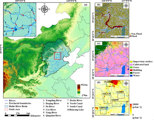
From the red polygon in Figure 1(a), the study area is located in the hinterland of the Haihe River Basin. It encompasses a small portion of mountainous terrain in the northwest, with the majority of the area being composed of plains and hills. And it mainly contains the Daqing River System, Yongding River System, and Baiyang Lake, which is composed of several rivers. To compare the accuracy of flood inundation extraction methods, both flood and non-flood areas were uniformly delineated from images captured before and after flood events. Subsequently, a random sampling technique was employed to select samples for accuracy verification, with the distribution of these samples depicted in Figure 1(b). The study area is primarily characterized by a significant expanse of cultivated land, which holds the foremost position and is further complemented by a substantial coverage of impervious surfaces, as illustrated in Figure 1(c). In addition, the study area is densely populated, especially in some medium and large cities, as depicted in Figure 1(d).

2.1.2. Data

This article uses five types of data, including Sentinel-1, Sentinel-2, ALOS DEM, population density, and land use data belonging to the three categories. Satellite images are used to obtain information on the inundation extent of flooding, DEM is used to obtain information on the depth of flooding. Based on the information obtained above, combined with remote sensing product, we acquire information about the impact of hazard-bearing bodies. Five types of data are described in detail as follows:

• Sentinel-1 data: Sentinel-1 satellite, consisting of two satellites carrying C-band SAR providing continuous imagery (day, night, and all types of weather), is an Earth observation satellite in the European Space Agency’s Copernicus program (GMES). Sentinel-1 data contains four data types, commonly used single look complex (SLC) and ground range detected (GRD). The GRD data eliminates thermal noise to improve image quality compared to SLC data and can be used directly for classification.

• Sentinel-2 data: Sentinel-2 satellite is a high-resolution multispectral imaging satellite comprised of Sentinel-2A and -2B. Each Sentinel-2 satellite carries the same multi-spectral instrument. The instrument captures images in 13 bands covering visible light, near-infrared, and short-wave infrared. The Sentinel-1 and Sentinel-2 data used in this article are in detailly introduced in Appendix Table A1.

• ALOS DEM data: ALOS DEM data are acquired from the (ALOS) satellite phased-array L-band synthetic aperture radar (PALSAR), a sensor with three observation modes: high-resolution, scanning SAR, and polarization. The data have a horizontal and vertical accuracy of up to 12.5 m. It can be downloaded free of charge through the Earth Data website (https://search.asf.alaska.edu).

• Population density data: WorldPop is a global assessment of demographic data launched by the University of Southampton in October 2013(www.worldpop.org), which has been widely recognized. Among them, the United Nations-adjusted (UN-adjusted) counting dataset, is using the unconstrained top-down modelling method. This dataset is used in this article to obtain regional headcounts.

• Land use data: The GlobeLand30 dataset is an important result of the research project on remote sensing mapping and key technologies for global land cover under the National High Technology Research and Development Program (863 Program) of China. It covers the land area of 80° north-south latitude, including 10 major categories of land cover information, such as cultivated land, forests, and impervious surfaces. Currently, there are three versions: 2000, 2010, and 2020. The dataset can be downloaded and used free of charge (http://globallandcover.com), and the latest version, 2020, is utilized in this study. In addition, buildings in impervious surfaces are obtained using the building rooftop area dataset (Zhang et al. 2023,  Liu et al. 2023).

2.2. Methodology

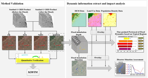
To grasp the ‘23.7’ BTH flood, this article established flood retrieving and analysis procedure, comprising three key components: a comparative comparison and selection of flood monitoring methods, the recreating of flood processes using retrieved flood dynamic information, and flood impact analysis based on hazard-bearing bodies. The specific workflow is depicted in Figure 2. Each component of the methodology is described in detail below.

Figure 2. Procedure of dynamic information extraction, flood evolution recreation, and impact analysis.

2.2.1. Flood mapping from SAR

Three recently published and exemplary multi-image-based flood extraction methods, namely FR (Nanditha et al. 2023), NDFI (Cian et al. 2018; Xue et al. 2022), and FZS (DeVries et al. 2020), were selected for comparative analysis with the author presented KDFIM. The detailed descriptions of these four methods are provided below.

FR method: Accumulated water, as a mirror surface with high reflectivity, has a lower backscatter value than dry surfaces. Before and after the flood, the ground surface changes from a dry surface to a specular surface and the backscattering changes. Nanditha et al. (2023) constructed the FR to obtain the extent of flooding by using the backscattering information from SAR: (1) $$\mathrm{\text{FR}}=\frac{\mathrm{\text{BFBS}}}{\mathrm{\text{AFBS}}}$$(1) where BFBS means before-flood backscatter information, AFBS means after-flood backscatter information.

FZS method: Ben DeVries et al. extracted the flood extent by calculating the FZS, which obtains flood information by calculating the VV backscatter correlation parameters. They defined the time period when no flooding occurred in the study area as the pre-event baseline boundary. Based on this, Sentinel-1 images were utilized to calculate the parameters of the FZS, that is, the time-averaged backscatter coefficient and the standard deviation backscatter coefficient (DeVries et al. 2020). The calculation formula is shown below: (2) $$\Delta {\sigma }_0^{p,m,d}\left(t\right)={\sigma }_0^{p,m,d}\left(t\right)-{\overline{\sigma }}_0^{p,m,d}$$(2) (3) $$Z^{p,m,d}\left(t\right)=\frac{\Delta {\sigma }_0^{p,m,d}\left(t\right)}{\mathit{\text{std}}\left({\sigma }_0^{p,m,d}\right)}$$(3) where p is polarization mode, m is sensor acquisition mode, and d is orbital direction. The individual parameters need to be at the same p, m, and d. ${\sigma }_0^{p,m,d}$ is the backscatter coefficient, ${\overline{\sigma }}_0^{p,m,d}$ is time-averaged backscatter coefficient, ${\mathit{\text{std}}(\sigma }_0^{p,m,d})$ is the standard deviation backscatter coefficient.

NDFI method: Time-series data can better portray the variation of each pixel of the ground surface. Normalized indexing can improve the efficiency of utilizing data by effectively compressing the information of long-time series data. Fabio Cian et al. construct two image sets, one containing only the reference image and the other also containing the image of the investigated flood, and later compute the NDFI to obtain the flood extent (Cian et al. 2018; Xue et al. 2022), as: (4) $$\mathrm{\text{NDFI}}=\frac{\mathrm{\text{mean}}{\sigma }_0\left(\mathrm{‘}\mathrm{\text{reference}}\mathrm{’}\right)-\mathrm{\text{min}}{\sigma }_0(\mathrm{‘}\mathrm{\text{reference}}+\mathrm{\text{flood}}\mathrm{’})}{\mathrm{\text{mean}}{\sigma }_0(\mathrm{‘}\mathrm{\text{reference}}’)+\mathrm{\text{min}}{\sigma }_0(\mathrm{‘}\mathrm{\text{reference}}+\mathrm{\text{flood}}\mathrm{’})}$$(4) where $\mathrm{\text{mean}}{\sigma }_0(\prime \mathrm{\text{reference}}\prime )$ is the average backscatter of the reference image set, $\mathrm{\text{min}}{\sigma }_0(\prime \mathrm{\text{reference}}+\mathrm{\text{flood}}\prime )$ is the minimum backscatter of the reference and flood image set.

KDFIM method: The KDFIM method extracts effective permanent water and flood features by fusing spatiotemporal information from SAR signals. It needs to calculate the microscopic characteristics before and after the flood, including permanent water features and flood features. The calculation of the microscopic characteristics of the flood is shown as follows:

To ensure the consistency of parameters for images before and after the flood, the image acquisition parameters should be rigorously controlled. Image parameter control is expressed through the following formula: (5) $${\sigma }_{f,j}={\sigma }_0^{d,a,p}\left(T_j\right)$$(5) where ${\sigma }_{f,j}$ is the j-th day’s flood microscopic characteristics after the flood, d is the orbital direction, a is the sensor acquisition mode, p is the polarization mode, ${\sigma }_0$ is the backscatter coefficient of VV polarization measured in decibels (dB), T_j is the j-th date of ${\sigma }_0$ after the flood.

The calculation method of the permanent water features is shown as: (6) $$s=\sum _{i=1}^n(t_i-t_0)$$(6) where s is the total number of rain-free days of all ${\sigma }_0$ before the flood, t_i is the i-th rain-free date of ${\sigma }_0$ before the flood, t₀ is the occurrence date of the flood. (7) $${\sigma }_{\mathit{\text{pw}},j}=\sum _{i=1}^n\frac{s-\Delta t_i}{2s}\mathrm{\hspace{0.17em}*\hspace{0.17em}}{\sigma }_0^{d,a,p}\left(t_j\right)$$(7) where ${\sigma }_{\mathit{\text{pw}},j}$ is the permanent water feature corresponding to the ${\sigma }_{f,j},$ d is the orbital direction, a is the sensor acquisition mode, p is the polarization mode, t_i is the i-th rain-free date of ${\sigma }_0$ before the flood, n is the total number of images with the same parameters before the flood.

Once the microwave characteristics before and after the flood are obtained, it is necessary to calculate the backscatter anomaly during the flood, as shown in Equation (8)(8) $${\Delta \sigma }_{f,j}={\sigma }_{f,j}-{\sigma }_{\mathit{\text{pw}},j}$$(8) . (8) $${\Delta \sigma }_{f,j}={\sigma }_{f,j}-{\sigma }_{\mathit{\text{pw}},j}$$(8) where ${\sigma }_{f,j}$ is the backscatter anomaly of the flood’s microscopic characteristics during the j-th date.

Comparison: In this article, to assess the effectiveness of the flood inundation extent method, four parameters are selected, namely Overall Accuracy (OA), Kappa coefficient (kappa), Omitted Error (E_O), and Committed Error (E_C) (Zhang et al. 2023). Their respective formulas are as follows: (9) $$\mathrm{\text{OA}}=(\mathrm{\text{TP}}+\mathrm{\text{TN}})/(\mathrm{\text{TP}}+\mathrm{\text{TN}}+\mathrm{\text{FP}}+\mathrm{\text{FN}})$$(9) (10) $$E_O=\mathrm{\text{FP}}/\mathrm{\text{TS}}$$(10) (11) $$E_C=\mathrm{\text{FN}}/\mathrm{\text{TS}}$$(11) (12) $$P_e=\frac{\left(\right(\mathrm{\text{TP}}+\mathrm{\text{FN}}\left)\mathrm{\hspace{0.17em}*\hspace{0.17em}}\right(\mathrm{\text{TP}}+\mathrm{\text{FP}})+(\mathrm{\text{TN}}+\mathrm{\text{FN}}\left)\mathrm{\hspace{0.17em}*\hspace{0.17em}}\right(\mathrm{\text{TN}}+\mathrm{\text{FP}}\left)\right)}{(\mathrm{\text{TP}}+\mathrm{\text{TN}}+\mathrm{\text{FP}}+\mathrm{\text{FN}})}$$(12) (13) $$\mathrm{\text{Kappa}}=(\mathrm{\text{OA}}-P_e)/(1-P_e)$$(13) where TP is the number of true floods classified as floods, FP is the number of true floods classified as non-floods, TN is the number of non-floods classified as non-floods, FN is the number of non-floods classified as floods, and TS is the total number of true floods in the reference map.

2.2.2. Extraction of flood dynamic information

The module is the knowledge-driven flood dynamic information calculation, which can compute flood height and shortest inundation duration. After obtaining the flood inundation area from threshold segmentation, other flood parameters can be further calculated. First of all, it is necessary to use boundary detection algorithms to obtain the boundary of the flood inundation extent (flood boundary). Afterward, the Elevations of the Flood Boundary (EFB) can be obtained by filtering the DEM values of the detected edges.

With the available EFB, we can further use the inverse distance weighted spatial interpolation to fit the Digital Surface Model of Flood (DSMF). The calculation formula is shown in Equation (14)(14) $$\mathrm{\text{DSMF}}=\sum _{h=1}^m\left[\frac{\mathit{\text{ST}}-S_h}{\left(m-1\right)\mathrm{\hspace{0.17em}*\hspace{0.17em}}\mathit{\text{ST}}}\mathrm{\hspace{0.17em}*\hspace{0.17em}}{\mathrm{\text{EFB}}}_h\right]$$(14) : (14) $$\mathrm{\text{DSMF}}=\sum _{h=1}^m\left[\frac{\mathit{\text{ST}}-S_h}{\left(m-1\right)\mathrm{\hspace{0.17em}*\hspace{0.17em}}\mathit{\text{ST}}}\mathrm{\hspace{0.17em}*\hspace{0.17em}}{\mathrm{\text{EFB}}}_h\right]$$(14) where DSMF is the digital surface model of the flooded area, ST is the total sum of distances to the near boundary points of the flood, S_h is the distance of the h-th near boundary points, EFB_h is the elevation of the h-th near boundary points, m is the number of points involved in the calculation.

After successfully fitting the flood DSMF, the final water depth of the flooded area can be obtained by conducting a subtraction operation with the original DEM. This determines the difference in elevation between the water surface and the surrounding terrain, providing valuable information about the depth of the flood. (15) $$\mathrm{\text{FH}}=\mathrm{\text{DSMF}}-\mathrm{\text{DEM}}$$(15) where FH is the local depth of the inundation area.

Afterward, at the pixel scale, time integration is carried out using water depth as a constraint to determine the duration of flood inundation. By incorporating water depth as an additional parameter, the analysis can filter out minor and less significant flood occurrences, allowing us to focus on areas with more substantial and prolonged inundation. Incorporating the water depth-based criterion enables a more refined and robust characterization of the flood dynamics, allowing for a more precise delineation of the actual flood-affected inundation. The detailed calculation method is as follows: (16) $$\mathrm{\text{FT}}=\sum _{j=1}^q\left[T_{j+1}\right(\mathrm{\text{FH}}>0)-T_j(\mathrm{\text{FH}}>0\left)\right]$$(16) where FT is the shortest duration of flood inundation, FH is the water depth and is utilized as a constraint to delimit the region involved in the calculation, Tj is the date of the j-th ${\sigma }_0$ since the flood, arranged in chronological order, q is the total number of acquired images since the flood.

2.2.3. Analysis of flood impact

This module utilizes existing remote sensing products including population density data and land use data combined with the retrieved flood information to count the number of affected populations, the area of impact building, and cultivated land. The calculation formulas are as follows: (17) $${\mathrm{\text{FB}}}_j=\sum _S{\Delta \sigma }_{f,j}\mathrm{\hspace{0.17em}*\hspace{0.17em}}B$$(17) where FB_j is the area of the impact building on the j-th date, ${\Delta \sigma }_{f,j}$ is the flood inundation of j-th date (0: non-flood, 1: flood), B is the building spatial distribution, S is the scope of the research area. (18) $${\mathrm{\text{FF}}}_j=\sum _S{\Delta \sigma }_{f,j}\mathrm{\hspace{0.17em}*\hspace{0.17em}}F$$(18) where FF_j is the area of flooded cultivated land on the j-th date, ${\Delta \sigma }_{f,j}$ is the flood inundation of j-th date (0: non-flood, 1: flood), F is the cultivated land spatial distribution, S is the scope of the research area. (19) $${\mathrm{\text{FP}}}_j=\sum _{\mathrm{S}}{\Delta \sigma }_{f,j}\mathrm{\hspace{0.17em}*\hspace{0.17em}}P$$(19) where FP_j is the number of people affected by the floods on the j-th date, ${\Delta \sigma }_{f,j}$ is the flood inundation of j-th date (0: non-flood, 1: flood), P is the population density spatial distribution, S is the scope of the research area.

3. Comparison of methods

3.1. Quantitative comparison of flood inundation

In this section, our primary objective is to quantitatively assess the accuracy and reliability of four algorithms, namely the NDFI, FZS, FR, and KDFIM. Subsequently, the optimal method is chosen for illustrating the progression of the ‘23.7’ BTH flooding process.

To ensure the reliability and comparability of the results, a total of 20,000 comparison samples were randomly selected, comprising 10,000 flood samples and 10,000 non-flood samples. The distribution of these samples is detailed in Figure 1(b). To assess the stability of each algorithm, a random sampling method was employed. From the 20,000 samples, 1000 samples (500 flood samples and 500 non-flood samples) were randomly selected for comparison. The accuracy metrics for each algorithm were averaged over 100 runs and summarized in Table 1. To obtain the best extraction results of flood, optimal thresholds for flood extraction were determined through repeated tests, as depicted in Figure 3. Additionally, to assess the stability of each algorithm, the standard deviation of the accuracy metrics over the 100 random samplings was calculated and presented in Figure 4.

Figure 3. Diagram of the calculation process of the optimal threshold for different indices.

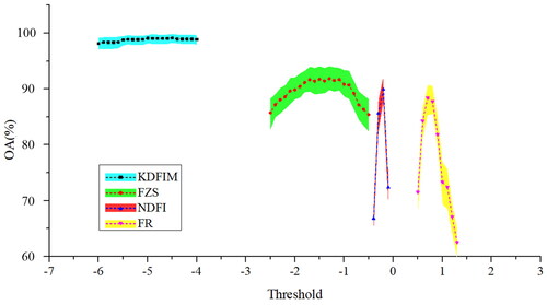
Figure 4. The standard deviation of quantitative comparison results of different methods.

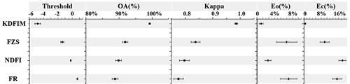
Table 1. The quantitative comparison of flood inundation results extracted with four methods.

Methods\metrics	OA	Kappa	EO	EC
NDFI	89.85%	0.7970	2.48%	17.82%
FR	88.78%	0.7755	7.15%	15.30%
FZS	91.87%	0.8374	6.68%	9.58%
KDFIM	99.26%	0.9853	0.93%	0.54%

In Figure 3, we chose for each method the segmentation threshold with the highest OA for its flood extraction results, ensuring fairness in the method comparison. It can be found that KDFIM can maintain high OA between −6 and −5, indicating that KDFIM has high stability and fault tolerance. The FZS method shows a slow-growing and decreasing trend between −2.5 and −0.5, and the highest OA occurs around −1.5. However, the FR and NDFI show a sharp growth of the decline, the thresholds can be selected in a very small range, and the fault tolerance is low.

From Table 1, it is evident that KDFIM outperforms the other methods, as it achieved the highest OA and Kappa values of 99.26% and 0.9853, along with the lowest E_O and E_C values of 0.93% and 0.54%, respectively. Following KDFIM, FZS also demonstrated strong performance with an OA exceeding 90%. In contrast, NDFI and FR yielded comparatively lower results, with OA values of 89.85% and 88.78%, respectively, primarily due to their higher E_C values of 17.82% and 15.30%, respectively.

To further analyze the stability of KDFIM, we conducted a repeated random sampling process and calculated the standard deviation of the accuracy evaluation metrics, as illustrated in Figure 4.

The horizontal float displayed in Figure 4 represents the standard deviation of the quantitative comparison results. The horizontal comparison reveals that there are significant fluctuations in FZS, NDFI, and FR, indicating low stability. Notably, both FZS and FR exhibit significant fluctuations in the E_O metric. It is important to highlight that KDFIM demonstrates better stability with minimal variations in its indicators. Moreover, KDFIM maintains high stability in both the OA and Kappa.

Furthermore, through a vertical comparison, it becomes evident that method instability primarily manifests in the Eo and Ec indicators, potentially leading to the omission of certain flood areas and misclassification of non-flood areas as flood areas. Notably, KDFIM exhibits clear advantages over other methods in terms of the Eo and Ec indicators, as depicted in Figure 3. On the other hand, the results of all methods are relatively stable when considering OA. To further confirm the accuracy of the quantitative comparison, this study proceeds to analyze the consistency of the overall flood inundation situation.

3.2. Comparison of inundation details

In this section, a comparative comparison of the results obtained from the NDFI, FR, FZS, and KDFIM methods for extracting the extent of flooding on August 5, 2023, was conducted, as depicted in Figure 5. The prominently highlighted red areas in the figure represent the extent of the flooded inundation.

Figure 5. Sentinel-1 Images: (a) image of July 24, 2023, before the flood; (b) image of August 5, 2023, during the flood; the flood inundation in red color on August 5, 2023, retrieved using (c) KDFIM, (d) FR, (e) NDFI, and (f) FZS, respectively.

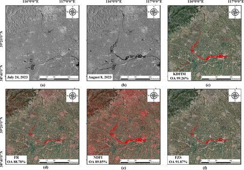
As shown in Figure 5, flash floods converge from the northwestern portion of the study area into the river and subsequently flow into the flood storage area. In addition, urban ponded water also converges towards the river, causing it to overflow and cause flooding. Comparing the results of the four methods in Figure 5(c)–(f), it can be observed that the extraction results of methods (d) FR, (e) NDFI, and (f) FZS exhibit noise and incorrectly identify areas like mountains and urban zones as flooded. Additionally, (d) FR and (f) FZS exhibit omission errors, failing to extract the floods within the flood storage area.

A comparative assessment of the accuracy and stability of the four methods showed that KDFIM had a significant advantage. The other three methods (FR, NDFI, and FZS) exhibit a common issue, which is increased noise resulting in the misclassification of many non-flood areas as floods. This phenomenon can be attributed to the sample scale problem. The flood-affected area represents a relatively small portion of the region, while the non-flood areas are much larger in extent. When using the same proportion of sample points, the limited characteristics of floods within the sample points fail to adequately differentiate non-flood areas from flood-affected ones. To ensure overall accuracy, a significant number of non-flood areas are mistakenly classified as floods.

From the previous section, the optimal segmentation thresholds for FR, NDFI, FZS, and KDFIM are 0.7, −0.2, −1.4, and −5, respectively. To eliminate the impact of sample point selection on the method comparison results, we have obtained the thresholds for FR, NDFI, and FZS mentioned in the original text of the methods to be 1.2, 0.7, and 0.6, respectively. Utilizing these thresholds, we have obtained the flood extraction results in DD (Figure 1) for these three methods, which are depicted in Figure 6.

Figure 6. Sentinel-1 Image on July 24, 2023, before the flood (a), on August 5, 2023, during the flood (b), and the flood inundation extraction on August 5, 2023 retrieved with a threshold of the method in this article, (c) FR, (e) NDFI, (g) FZS, with a threshold of the original method, (d) FR, (f) NDFI, and (h) FZS.

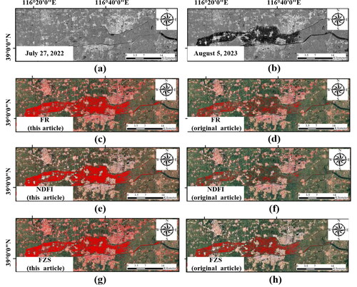
The results of the three methods, FR, NDFI, and FZS, under the optimal thresholds, are compared with those under the thresholds in the original method in Figure 6(a)–(h). It is revealed that the noise-induced incorrect scores are significantly lower in the latter, but at the same time, a large number of missed scores occur. In both scenarios, KDFIM is the most optimal choice. Therefore, it does not affect the results of this paper.

In conclusion, KDFIM effectively avoids noise-induced misclassification such as mountain superimpositions and city spots. It has the highest accuracy and reliability compared with others three algorithms.

4. ‘23.7’ BTH flood evolution

4.1. General evolution of ‘23.7’ BTH flood-inundation

In this section, the primary objective is to capture the temporal evolution of flood inundation extent and depth using the KDFIM method. Specifically, water depths in the flood-affected areas are computed on five distinct dates: August 5, 2023, August 17, 2023, August 29, 2023, September 10, 2023, and September 22, 2023, as illustrated in Figure 7(a)–(e). The intrinsic errors within DEM data, which cannot be entirely eradicated (https://search.asf.alaska.edu/#/), result in the determination of the error of our current water depth results through the error transfer formula, yielding a calculated error of 2 m.

Figure 7. Flooded zone in the study area extracted with KDFIM on (a) August 5, 2023, (b) August 17, 2023, (c) August 29, 2023, (d) September10, 2023, (e) September22, 2023, respectively.

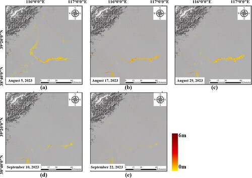
Figure 7(a)–(e) illustrate the progression of flooding from August 5 to September 22. It is apparent that on August 5, there was flooding in the river and the flood extent in the flood storage area was substantial. By August 17, the flooding in the river had diminished, and flooding in the central north-south direction of the flood storage area had receded. On August 29, there was minimal flooding in the channel, and the depth of flooding in the east-west direction of the flood storage area was decreased. Both September 10 and September 22 witnessed a further reduction in the extent and depth of flooding.

Consequently, the evolution of the flooding process can be discerned. From July 29 to August 5, urban water from city pipelines and upstream flash floods continued to flow into the river, gradually reducing urban flooding. Between August 5 and August 29, the flooding gradually converged into the flood storage area, while the river steadily decreased until it vanished. The flood area within the flood storage area initially expanded and then contracted, and the water depth followed a pattern of initial increase and subsequent decrease.

4.2. Details of ‘23.7’ BTH flood-inundation

To provide a more comprehensive and detailed depiction of the flood’s progression, this section further concentrates on five typical regions (as displayed in Figure 1d). The obtained flood parameter values, including the area of flood inundation, and water depths for these representative regions on August 5, 2023, August 17, 2023, August 29, 2023, September 10, 2023, and September 22, 2023, are presented in Figure 8(a)–(y).

Figure 8. Detailed information of the flooded area in BYLF (a–e), LGW (f–j), DD (k–o), MTG (p–t), and YDF (u–y) on (a) August 5, 2023, (b) August 17, 2023, (c) August 29, 2023, (d) September 10, 2023, and (e) September 22, 2023, respectively.

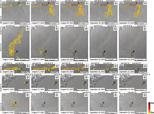
In addition, this section compiles data on the changes in flood-affected areas for the five mentioned dates, as depicted in the bar charts on the left side of Figure 9(a)–(e). Furthermore, we have selected one land-use category from each of these regions to track the variations in water depth, enhancing our understanding of the flood’s progression, as illustrated in the bar charts on the right side of Figure 9(a)–(e). The smaller regions in Figure 9 display the water depth dynamic results for the chosen land-use categories. And their geographic locations correspond to the black identifiers in Figure 8.

Figure 9. The change of total inundation area and water depth in (a) BYLF, (b) LGW, (c) DD, (d) MTG, and (e) YDF from August 5, 2023 to September 22, 2023.

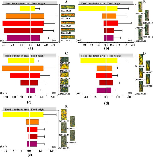
Being evident in Figure 8(a)–(e) and the left side of Figure 9(a), the extent of flooding inundation at BYLF gradually increased from a small amount on August 5 to a maximum of approximately 30 km² on August 29. Subsequently, a receding phenomenon occurred, accompanied by a slow reduction in flooding. The right side of Figure 9(a) displays the variation in water depth at the entrance of BYLF. It is notable that the water depth was 0.6 m on August 5, peaked at 1.8 m on August 17, and then gradually decreased to 1.2 m by September 22.

Extensive flooding was observed in LGW on August 5, covering an area of approximately 75 km². By August 17, this area had significantly reduced to about 10 km², particularly in the northern part where the flooding had almost disappeared. Subsequently, minor floods of 5.6, 4.0, and 4.7 km² were recorded on August 29, September 10, and September 22, respectively, as shown in the left side of Figure 8(f)–(j) and Figure 9(b). On the right side of Figure 9(b), the variation in water depth in some agricultural fields within LGW is depicted. There is minimal variation in water depth there, with all water depths around 1 m. On August 17, the overall extent of flooding in the region had decreased, but the maximum water depth reached 1.1 m on August 29.

Observing Figure 8(k)–(o) and the left side of Figure 9, it is evident that DD experienced extensive flooding on August 5, covering an area of approximately 132 km². The extent of flooding peaked at 170 km² on August 17, primarily due to the discharge of floodwaters from LGW into DD. Subsequently, the flooding rapidly receded, nearly disappearing by September 22. On the right side of Figure 9(c), the variation in water depth in some agricultural fields within DD exhibits an initial increase followed by a decrease. The minimum water depth was 0.4 m on August 5, reaching a maximum of around 1.2 m on August 17, and subsequently decreasing to 0.5 m by September 22.

In Figure 8(p)–(t) and (u)–(y), MTG and YDF are depicted, both of which are situated within the floodplain of the Yongding River System. MTG is located upstream, while YDF is downstream. It is noticeable that both regions experienced their maximum flood extents of 5 and 14 km² on August 5, and their minimum extents of 1.3 and 0.5 km² on September 10, respectively. The right side of Figure 9(d) and (e) illustrate the variation of water depth in the wetland area of MTG and the village area of YDF, accordingly. It can be found that the same they both have maximum water depths of 1 m and 1.2 m on August 5, separately. Both of them have little change in water depth, about 0.5 and 0.6 m respectively.

A systematic review referring to the geographical location in the basin and the spatio-temporal difference in regional rainfall is presented. Extreme precipitation since July 29 resulted in river surges and flooding in the basin until September 22, when the flooding subsided. Continuous rainfall led to widespread water accumulation across the entire watershed and plains, particularly causing flash floods in areas with intense precipitation. Before August 5, the Yongding River System was affected by precipitation and flash floods occurred rapidly, with the upstream MTG being the first to flood due to its proximity to the mountainous areas, and the residual flash floods and urban floods pooled in the downstream YDF and then gradually disappeared. To mitigate the disaster, the DD and LGW flood storage zones in the Daqing River System were activated before August 5, so that urban floods and flash floods gradually converged to the storage zones and receded by September 22. Floods in the BYD, which were converged by the upstream rivers, came late on August 5, and stagnated due to the structure of the watershed in this area.

4.3. Dynamic impacts of the flood-inundation

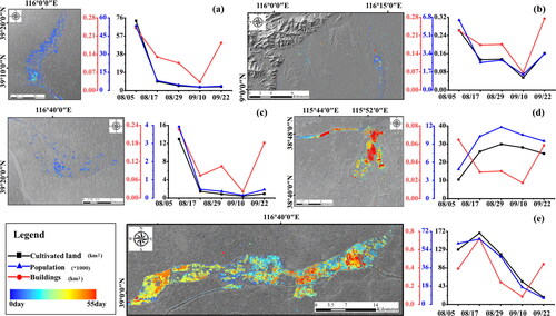
Floods pose a significant threat to both human lives and property. They not only inundate homes but also carry away all the possessions in settlements, and submerge cultivated land, leading to the destruction of crops and a significant reduction in food production. In this section, the shortest inundation duration of floods (Figure 10) and the time-series variation of the number of affected populations, the area of flooded building, and cultivated land in five typical areas are obtained to analyze the impact of floods, as depicted in Figure 11. The line charts on the right side of Figure 11(a)–(e) illustrate the variations in the impact of flooding on the population, the area of cultivated land, and the area of building in each region on August 5, August 17, August 29, September 10, and September 22.

Figure 10. Distribution map of flood shortest inundation duration.

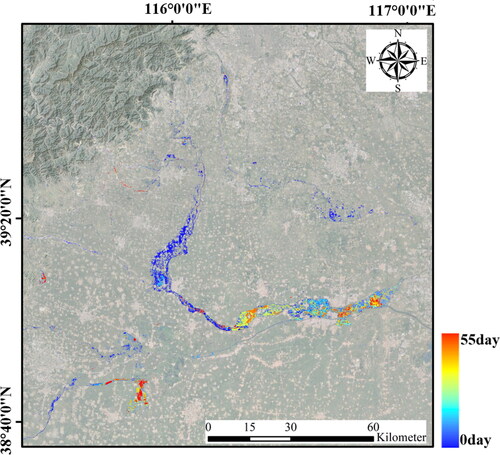
Figure 11. Duration of the flood inundation and the change of affected population (*1000), impervious surface (km²), and cultivated land (km²) inside (a) LGW, (b)MTG, (c) YDF, (d) BYLF, and (e) DD, respectively.

Based on the comprehensive flood shortest inundation duration map in Figure 10 and the distribution of typical areas in Figure 11, it is evident that the area with the longest flood shortest inundation duration is primarily BYLF in the southwest, lasting for approximately 30 days. It is followed by the central flood storage area DD, enduring for around 26 days. In contrast, the Yongding River System (MTG, YDF) and the flood storage area LGW in the north experience shorter inundation periods, ranging from 9 to 16 days.

The analysis of the impact situation in the five typical regions is presented below. As depicted in the right-hand line graph in Figure 11(a), it is evident that the LGW region faced the most severe impact on August 5, affecting a total of 53,393 people, 72.94 km² of cultivated land area, and 0.25 km² of building area. Subsequently, the population and the area of cultivated land showed a significant decrease in these figures until September 10 with 2969 and 3.61 km² respectively.

The line graphs on the right side of Figure 11(b) MTG and Figure 11(e) YDF reveal that in the Yongding River System, also experienced a significant impact on August 5. In the MTG region, the number of people affected reached as high as 6534, with 0.26 km² of cultivated land area and 0.23 km² of building area. Subsequently, the impact decreased to its lowest level on September 10, with the number of affected people reduced to 1452, 0.06 km² of affected cultivated land area, and 0.07 km² of building area. In the YDF region, on August 5, 3930 people, 12.97 km² of cultivated land area, and 0.23 km² of building area were affected. On September 10, the disaster situation reached its lowest point, with the number of affected people reduced to 1500, 0.43 km² of affected cultivated land area, and 0.02 km² of building area.

In the DD region (Figure 11e), the largest affected cultivated land area, covering 168.51 km², was observed on August 17th, with the highest number of affected people and building area of 60,187 and 0.39 km², respectively. Meanwhile, on September 10, the affected building area was the smallest, with 0.09 km². On September 22, the least affected population, and the smallest cultivated land area, with 6170 and 16.87 km², respectively.

For the BYLF area (Figure 11d), the trend of the population and cultivated land area affected by flooding shows a general pattern of increasing and then decreasing, with peaks of 11,810 and 29.94 km² of affected population and cultivated land area, respectively, on August 29. In contrast, the affected building area had a maximum value of 0.06 km² on August 5. This is due to the distribution of the buildings. Although the inundation area of the flood was not large on August 5, a large number of buildings happened to be present in the inundation area.

It is worth noting that all five regions experienced an increase in impact on September 22, likely due to additional rainfall during that period.

5. Conclusions

This article recreates the ‘23.7’ BTH flood by constructing a flood retrieving and analysis procedure, revealing flood inundation extant, water depth, and shortest inundation duration. The revealed impact information of floods on hazard-bearing bodies serves to illuminate the development of floods, laying bare both the instantaneous destruction and the protracted inundation.

The flood event commenced on July 29 and had largely dissipated by September 22. Notably, the accumulation of water in urban areas and the convergence of flash floods on August 5 resulted in the largest flood inundation extent in the detention basin, with subsequent recession. Specifically, the evolution of floods in different regions is not uniform. Floods were first seen in MTG, closer to the mountains, and flowed rapidly to the Yongding River floodplain, where it subsided rapidly. For the flood storage area in the Daqing River System, the LGW in the upstream flowed rapidly to the DD in the downstream and receded slowly. In contrast, flooding in the BYD region appeared the latest, with stagnation of floodwaters. It is worth noting that the water depth reached up to 6 m, and the shortest inundation duration extended to as long as 30 days, significantly affecting the livelihoods and production activities of the residents.

Through the reappearance and analysis of this flood event, it can be concluded that flood control projects should be planned more rationally based on information regarding terrain and land types. For example, in the transition zone between mountainous and plain areas in BTH, strengthening the construction of flood control facilities would further enhance the ability to cope with catastrophic floods.

Disclosure statement

No potential conflict of interest was reported by the author(s).

Additional information

Funding

This study is partly supported by the National Key Research and Development Program of China under Grant 2023YFE0208000, the Key Program of the National Natural Science Foundation of China (NSFC) under Grant 41930108, Fundamental Research Funds for the Central Universities of Central South University under Grant 2024ZZTS0369; and the National Natural Science Foundation of China (NSFC) under Grant 42071256.

Appendix

Table A1. List of Sentinel-1 and Sentinel-2 scenes used, the image identifier, the date, the pass direction of satellite.

	Satellite	Image Identifier	Date	Pass direction
Before flood	S-1	S1A_IW_GRDH_1SDV_20220729T101404_20220729T101429_044314_0549E2_3F89	2022/07/29	ASCENDING
	S-1	S1A_IW_GRDH_1SDV_20220729T101339_20220729T101404_044314_0549E2_ACB5	2022/07/29	ASCENDING
	S-1	S1A_IW_GRDH_1SDV_20230712T101408_20230712T101433_049389_05F067_27AC	2023/07/12	ASCENDING
	S-1	S1A_IW_GRDH_1SDV_20230712T101343_20230712T101408_049389_05F067_566A	2023/07/12	ASCENDING
	S-1	S1A_IW_GRDH_1SDV_20230724T101409_20230724T101434_049564_05F5BB_DFA6	2023/07/24	ASCENDING
	S-1	S1A_IW_GRDH_1SDV_20230724T101344_20230724T101409_049564_05F5BB_58D9	2023/07/24	ASCENDING
Amidst a flood	S-2	S2A_MSIL2A_20230802T025531_N0509_R032_T50SMJ_20230802T061154	2023/08/02	ASCENDING
	S-1	S1A_IW_GRDH_1SDV_20230805T101410_20230805T101435_049739_05FB20_B9E4	2023/08/05	ASCENDING
	S-1	S1A_IW_GRDH_1SDV_20230805T101345_20230805T101410_049739_05FB20_5BBD	2023/08/05	ASCENDING
	S-1	S1A_IW_GRDH_1SDV_20230817T101345_20230817T101410_049914_0600FF_C86A	2023/08/17	ASCENDING
	S-1	S1A_IW_GRDH_1SDV_20230817T101410_20230817T101435_049914_0600FF_23C8	2023/08/17	ASCENDING
	S-1	S1A_IW_GRDH_1SDV_20230829T101411_20230829T101436_050089_060703_F906	2023/08/29	ASCENDING
	S-1	S1A_IW_GRDH_1SDV_20230829T101346_20230829T101411_050089_060703_741D	2023/08/29	ASCENDING
	S-1	S1A_IW_GRDH_1SDV_20230910T101412_20230910T101437_050264_060CF4_CA2A	2023/09/10	ASCENDING
	S-1	S1A_IW_GRDH_1SDV_20230910T101347_20230910T101412_050264_060CF4_D222	2023/09/10	ASCENDING
	S-1	S1A_IW_GRDH_1SDV_20230922T101412_20230922T101437_050439_0612EA_E557	2023/09/22	ASCENDING
	S-1	S1A_IW_GRDH_1SDV_20230922T101347_20230922T101412_050439_0612EA_A46D	2023/09/22	ASCENDING

References

- Chini M, Hostache R, Giustarini L, Matgen P. 2017. A hierarchical split-based approach for parametric thresholding of SAR images: flood inundation as a test case. IEEE Trans Geosci Remote Sensing. 55(12):6975–6988. doi: 10.1109/TGRS.2017.2737664.
- Cian F, Marconcini M, Ceccato P. 2018. Normalized difference flood index for rapid flood mapping: taking advantage of EO big data. Remote Sens Environ. 209:712–730. doi: 10.1016/j.rse.2018.03.006.
- DeVries B, Huang C, Armston J, Huang W, Jones JW, Lang MW. 2020. Rapid and robust monitoring of flood events using Sentinel-1 and Landsat data on the Google Earth Engine. Remote Sens Environ. 240:111664. doi: 10.1016/j.rse.2020.111664.
- Du X, He B, Xu W, Zhang M, River YDH. 2023. “23-7” Basin flood storage and stagnation floodplain utilization review and thinking on green development of system governance. Flood Control and Drought Relief in China. 33(09):31–38.
- Feng P, Wu J, Li J. 2019. Changes in flood characteristics and the flood driving mechanism in the mountainous Haihe River Basin, China. Hydrol Sci J. 64(16):1997–2005. doi: 10.1080/02626667.2019.1619931.
- Fu J, Zang C, Zhang J. 2020. Economic and resource and environmental carrying capacity trade-off analysis in the Haihe River Basin in China. J Cleaner Prod. 270:122271. doi: 10.1016/j.jclepro.2020.122271.
- Giustarini L, Hostache R, Matgen P, Schumann GJP, Bates PD, Mason DC. 2013. A change detection approach to flood mapping in urban areas using TerraSAR-X. IEEE Trans Geosci Remote Sensing. 51(4):2417–2430. doi: 10.1109/TGRS.2012.2210901.
- Güneralp B, Güneralp İ, Liu Y. 2015. Changing global patterns of urban exposure to flood and drought hazards. Global Environ Change. 31:217–225. doi: 10.1016/j.gloenvcha.2015.01.002.
- Ki-Moon B. 2015. Secretary-General’s remarks at launch of the 2015 Global assessment report on disaster risk reduction: making development sustainable – The future of disaster risk management.
- Kundzewicz ZW, Huang J, Pinskwar I, Su B, Szwed M, Jiang T. 2020. Climate variability and floods in China - A review. Earth Sci Rev. 211:103434. doi: 10.1016/j.earscirev.2020.103434.
- Kundzewicz ZW, Kanae S, Seneviratne SI, Handmer J, Nicholls N, Peduzzi P, Mechler R, Bouwer LM, Arnell N, Mach K, et al. 2014. Flood risk and climate change: global and regional perspectives. Hydrol Sci J. 59(1):1–28. doi: 10.1080/02626667.2013.857411.
- Landuyt L, Coillie FMBV, Vogels B, Dewelde J, Verhoest NEC. 2021. Towards operational flood monitoring in Flanders using Sentinel-1. IEEE J Sel Top Appl Earth Observ Remote Sensing. 14:11004–11018. doi: 10.1109/JSTARS.2021.3121992.
- Liu Z, Tang H, Feng L, Liu S. 2023. China building rooftop area: the first multi-annual (2016–2021) and high-resolution (2.5 m) building rooftop area dataset in China derived with super-resolution segmentation from Sentinel-2 imagery. Earth Syst Sci Data. 15(8):3547–3572. doi: 10.5194/essd-15-3547-2023.
- Luo K, Zhang X. 2022. Increasing urban flood risk in China over recent 40 years induced by LUCC. Landscape Urban Plann. 219:104317. doi: 10.1016/j.landurbplan.2021.104317.
- Mahmoud S, Gan TY. 2018. Urbanization and climate change implications in flood risk management: developing an efficient decision support system for flood susceptibility mapping. Sci Total Environ. 636:152–167. doi: 10.1016/j.scitotenv.2018.04.282.
- Mason DC, Horritt MS, Dall’Amico JT, Scott TR, Bates PD. 2007. Improving river flood extent delineation from synthetic aperture radar using airborne laser altimetry. IEEE Trans Geosci Remote Sensing. 45(12):3932–3943. doi: 10.1109/TGRS.2007.901032.
- Mason DC, Speck R, Devereux B, Schumann GJP, Neal JC, Bates PD. 2010. Flood Detection in Urban Areas Using TerraSAR-X. IEEE Trans Geosci Remote Sensing. 48(2):882–894. doi: 10.1109/TGRS.2009.2029236.
- Matgen P, Hostache R, Schumann G, Pfister L, Hoffmann L, Savenije HHG. 2011. Towards an automated SAR-based flood monitoring system: lessons learned from two case studies. Phys Chem Earth Parts A/B/C. 36(7–8):241–252. doi: 10.1016/j.pce.2010.12.009.
- Mehravar S, Seyed VR, Armin M, Babak R, Fatemeh F, Meisam A. 2023. Flood susceptibility mapping using multi-temporal SAR imagery and novel integration of nature-inspired algorithms into support vector regression. J Hydrol. 617:129100. doi: 10.1016/j.jhydrol.2023.129100.
- Nanditha JS, Kushwaha AP, Singh R, Malik I, Solanki H, Chuphal DS, Dangar S, Mahto SS, Vegad U, Mishra V, et al. 2023. The Pakistan flood of August 2022: causes and Implications. Earth’s Future. 11(3):e2022EF003230. doi: 10.1029/2022EF003230.
- Qi XJ, Wang DZ, Zhong W, Xiao F, Li SS. 2024. A comparative analysis of the Yongding River flood in 2023 and the historical rainstorm flood in 1939. China Water Resources. 03:65–68.
- Schumann GJ, Bates PD, Apel H, Aronica GT. 2018. Global Flood Hazard: applications in modeling, mapping and forecasting. Washington (DC): American Geophysical Union- Standards Information Network.
- Shastry A, Carter E, Coltin B, Sleeter R, McMichael S, Eggleston J. 2023. Mapping floods from remote sensing data and quantifying the effects of surface obstruction by clouds and vegetation. Remote Sens Environ. 291:113556. doi: 10.1016/j.rse.2023.113556.
- Thomas M, Tellman E, Osgood DE, DeVries B, Islam AS, Steckler MS, Goodman M, Billah M. 2023. A framework to assess remote sensing algorithms for satellite-based flood index insurance. IEEE J Sel Top Appl Earth Observ Remote Sensing. 16:2589–2604. doi: 10.1109/JSTARS.2023.3244098.
- Torres R, Snoeij P, Geudtner D, Bibby D, Davidson M, Attema E, Potin P, Rommen B, Floury N, Brown M, et al. 2012. GMES Sentinel-1 mission. Remote Sens Environ. 120:9–24. doi: 10.1016/j.rse.2011.05.028.
- Ward DP, Petty A, Setterfield SA, Douglas MM, Ferdinands K, Hamilton SK, Phinn S. 2014. Floodplain inundation and vegetation dynamics in the Alligator Rivers region (Kakadu) of northern Australia assessed using optical and radar remote sensing. Remote Sens Environ. 147:43–55. doi: 10.1016/j.rse.2014.02.009.
- Xu H, Duan Y, Xu X. 2022. Indirect effects of binary typhoons on an extreme rainfall event in Henan Province, China from 19 to 21 July 2021: 1. Ensemble-based analysis. J Geophys Res Atmos. 127:e2021.
- Xue F, Gao W, Yin C, Chen X, Xia Z, Lv Y, Zhou Y, Wang M. 2022. Flood monitoring by integrating normalized difference flood index and probability distribution of water bodies. IEEE J Sel Top Appl Earth Observ Remote Sensing. 15:4170–4179. doi: 10.1109/JSTARS.2022.3176388.
- Yao J, Sun S, Zhai H, Feger K-H, Zhang L, Tang X, Li G, Wang Q. 2022. Dynamic monitoring of the largest reservoir in North China based on multi-source satellite remote sensing from 2013 to 2022: water area, water level, water storage and water quality. Ecol Indic. 144:109470. doi: 10.1016/j.ecolind.2022.109470.
- Yao W. 2023. Digitally empowering the prevention of catastrophic floods in the “23.7” Haihe River Basin. China Water Conservancy. 18:13–18.
- Zhang Z, Fan Y, Jiao Z, Fan B, Zhou J, Li Z. 2023. Vegetation ecological benefits index (VEBI): a 3D spatial model for evaluating the ecological benefits of vegetation. Int J Digital Earth. 16(1):1108–1123. doi: 10.1080/17538947.2023.2192527.