Evaluation of groundwater-caused deformation patterns in a metropolitan area using time series InSAR and retrieval of vertical and east-west displacement: a case study in Taipei City

Abstract

This study explores the influences of groundwater fluctuations in an urban area which lead to long-term ground surface subsidence using a time-series synthetic aperture radar interferometry (InSAR) technique. Unlike most prior studies that only focus on line-of-sight (LOS) deformation, assume negligible horizontal movements, and quantify InSAR-groundwater relationship on a sparse temporal scale, this study utilized the Persistent Scatterers InSAR (PS-InSAR) technique to extract east-west and vertical displacement by decomposing Sentinel-1 ascending and descending datasets spanning from 2018 to 2022. Additionally, an approach was proposed to effectively quantify the relationship between changes in groundwater levels and vertical displacement on a daily basis. The results underwent robust validation against ground-based leveling surveys, revealing a satisfactory NRMSE of 1.06 mm/yr. Furthermore, founded on the estimated vertical displacement, three districts within Taipei City (e.g. Wugu, Xinzhuang, and Taishan) were identified as subsidence hotspots, with maximum vertical deformation rates reaching −11.77 mm/yr. Eventually, the correlation analysis and quantification between vertical displacement and daily groundwater data underscore long-term groundwater fluctuations as the primary cause of subsidence. These findings, derived from InSAR-based 2D displacements, have proven valuable in understanding groundwater-caused ground subsidence hazards in urban areas and empowering relevant stakeholders to set out corresponding adaptation and mitigation measures.

Keywords:

• Persistent scatterers InSAR (PS-InSAR)
• 2D displacement analysis
• sentinel-1A
• urban land subsidence monitoring
• geodetic leveling survey
• groundwater well observation
• groundwater depletion
• urban aquifer-land surface dynamics

1. Introduction

Land subsidence is often caused by the over-utilization of groundwater. According to the United Nations Educational, Scientific and Cultural Organization (UNESCO) land subsidence model, one-fifth of the global population is projected to experience land subsidence by 2040 due to groundwater depletion (Herrera-García et al. 2021). Rapid urban development to meet the increasing demands for infrastructure, housing, and transportation systems has disrupted the natural ecosystem (Dixon et al. 2006). This unprecedented development often triggers severe floods and runoff situations due to inefficient groundwater management. Unsustainable groundwater extraction depletes aquifers, leading to soil layer compression when the rate of aquifer depletion surpasses the rate of replenishment. A decline in the groundwater level raises pore water pressure, causes an inverse impact on the effective stress of the surface (Terzaghi, 1925) and eventually results aquifer compaction as well as surface deformation (Galloway and Burbey, 2011). Such processes pose substantial risks to underground infrastructure, buildings, bridges, railways, and canals (Leake, 2016). Depending on the pre-consolidation stress in soil sediments, aquifer compaction involves both elastic and inelastic phenomena, with the former recoverable over time and the latter irreversible. Instances of groundwater-related subsidence have been reported globally in urban centers, including China (Zhang et al. 2014; Hu et al. 2022; Li et al. 2022), Mexico (Castellazzi et al. 2021; Cigna and Tapete, 2021), India (Awasthi et al. 2022; Garg et al. 2022; Kim et al. 2023), and Taiwan (Tung et al. 2016; Chen et al. 2023). According to UNESCO’s report (Herrera-García et al. 2021), over 200 locations in 34 countries have experienced land subsidence due to excessive groundwater withdrawal. Therefore, it is crucial to comprehend the correlation between land subsidence and groundwater for understanding spatiotemporal variations and making predictions for the future.

Numerous methods, such as leveling, extensometers, and the Geographic Positioning System (GPS) (Metzger et al. 2001; Zhang et al. 2014), have been employed in the past to measure groundwater-related subsidence. These methods offer relative surface elevation changes concerning a presumed stable reference point, establishing a qualitative relationship between surface deformation and groundwater data at discrete locations (Galloway and Burbey, 2011). Over the past few decades, the InSAR technique has been developed to provide large-scale ground deformation measurement with high spatio-temporal precision. The potential of InSAR tool has been explored across various application domains encompassing tunneling, railways, and subsidence monitoring in metropolitan areas (Solano-Rojas et al. 2020; Chen et al. 2021; Cigna and Tapete, 2021; Ramirez et al. 2022). Additionally, InSAR based land subsidence measurements offer an alternative method for estimating piezometric head in confined aquifers (Galloway and Burbey, 2011; Chen et al. 2017). Conventional InSAR measurements are adversely affected by signal de-correlations in both spatial and temporal dimensions (Zebker and Villasenor, 1992), as well as atmospheric effects (Zebker et al. 1997), which are challenging to compensate effectively. The development of time series InSAR techniques, such as PS-InSAR (Ferretti et al. 2001) and small baseline subsets (SBAS) (Berardino et al. 2002), has effectively addressed these limitations. Utilizing extensive temporal series of InSAR images, these advanced techniques extract surface deformation over time with millimetric accuracy (Rucci et al. 2012). In general, InSAR measurements are conducted in the 1D LOS direction. Nevertheless, this constraint can be addressed by integrating both ascending and descending InSAR observations, and subsequently decomposing them into vertical and horizontal deformations (Eriksen et al. 2017).

In order to utilize these techniques, Bell et al. (2008) employed PS-InSAR technique to evaluate the seasonal impact of groundwater pumping on aquifer related compaction from 1992 to 2005 in Las Vegas Valley, Nevada. Tung et al. (2016) investigated the spatio-temporal variations, co-relating InSAR and groundwater measurements in the Taipei basin, to estimate aquifer storativity (S) and characterize potential subsidence. Examining aquifer compaction, Liu et al. (2018) with the help of PS-InSAR observations differentiated between elastic and inelastic deformation, associating high storativity with inelastic deformation. Nevertheless, surface deformation caused by groundwater withdrawal propagates not only vertically but also horizontally across the land surface (Galloway and Burbey, 2011). To investigate the mechanism, Burbey et al. (2006) conducted a 60-day aquifer test in Mesquite, Nevada, and observed angularly varying deformations using GPS-based horizontal and vertical measurements. Following this, Ye et al. (2016) developed a 3D geo-mechanical model in Shanghai metropolitan area, integrating groundwater flow and aquifer-based displacement observations. They concluded that horizontal displacement occurred in the urban core and suggested InSAR could enhance understanding between the two observations. Furthermore, InSAR-derived 3D deformation is crucial for assessing spatiotemporal consistency and correlations with fluctuations in groundwater levels. Consequently, Rezaei and Mousavi (2019) computed deformation in each direction using InSAR based ENU-decomposition techniques. However, they derived aquifer parameters for Iran’s Gorgan confined aquifer by assuming similarity between vertical (U) and LOS deformation, neglecting horizontal deformations. The LOS incidence to vertical, assuming no horizontal motions, serves as an alternative method for estimating vertical deformation. This is a commonly employed method for the spatio-temporal evaluation of land subsidence, as frequently implemented in several research works (Dong et al. 2021; Garg et al. 2022; Ramirez et al. 2022).

Nevertheless, this assumption can sometimes introduce significant error depending on the existence of horizontal deformation and the angle of incidence of LOS (Fuhrmann and Garthwaite, 2019). Furthermore, establishing a quantitative relationship between groundwater and InSAR requires that purely vertical ground deformation (U) correlates with the hydraulic head change and allows for the calculation of the storativity parameter, which characterizes the aquifer’s compressibility (Riley, 1969). Therefore, the optimal approach for precise estimates involves combining multiple viewing LOS InSAR observations to derive 3D East-North-Up (ENU) deformation and extracting the displacement time series in each direction (Hu et al. 2014). However, previous studies often overlooked this aspect and primarily relied on vertical deformation derived from incident LOS deformation using either ascending or descending datasets. This approach left one of the datasets underutilized, and integrating both could offer comprehensive 3D deformation dynamics. Moreover, even though groundwater well data could typically be accessed at daily temporal resolution, allowing for a comprehensive assessment of long-term temporal dynamics, they have not been extensively exploited. Consequently, to overcome these limitations, comprehend the spatio-temporal dynamics, and further develop a robust quantitative relationship between vertical displacement and groundwater level change, the main objective of this research involves: (1) first robust time series InSAR processing in Taipei and New Taipei metropolitan areas to assess deformation patterns using 4.5 years of Sentinel-1 datasets, (2) estimation of vertical and east-west displacement time series to extract the actual displacement in each dimension, (3) global validation of InSAR-derived vertical deformation against the Taipei leveling network, assessing robustness through statistical evaluation, and (4) formulation of an alternative methodology to exploit the quantitative relationship between InSAR and daily groundwater well measurement.

2. Study area

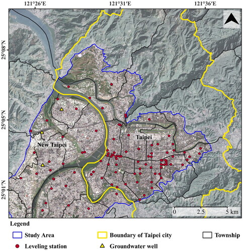
Taipei, the capital of Taiwan, forms the special municipality and is one of the densest metropolitan areas in northern Taiwan. In 2010, a significant portion of Taipei underwent a renaming process and was formally established as New Taipei. This new entity has since become one of Taiwan’s largest municipalities in terms of geographical area. The study area, that is Taipei Basin, one of the most unique geomorphic features in northern Taiwan, comprising the main urban metropolis of Taipei and New Taipei, covering approximately 250 km², as illustrated in Figure 1. Situated on the ancient lakebed of the Taipei basin, the urban area is encircled by mountains and bordered to the east by the Keelung Valley and to the south by the Xindian River, which converges with the Tamsui River to the west.

Figure 1. The geographical locations of the study area as the well as leveling and groundwater well stations, shown on the Sentinel-2A image acquired on 2022/7/24 overlaid on a shaded relief map.

The geological conditions in the Taipei Basin exhibit significant diversity, characterized by hilly and mountainous terrain encompassing the area from all directions. The landscape is primarily composed of Quaternary alluvio-lacustrine sediment, alongside the gradual accumulation of alluvial fans, fluvial plains, and estuaries since about 0.4 Ma (Teng et al. 2001). Quaternary deposits are classified into four lithostratigraphic layers, namely the Sungshan, Jingmei, Wuku, and Banchiao formations, arranged from top to bottom (Teng et al. 1999). These formations constitute the aquifer system of the basin. The Sungshan formation, located at the top, comprises an unconfined aquifer primarily replenished by rainfall. In contrast, the Jingmei formation, densely packed both above and below, represents a confined aquifer. According to Chia et al. (1999), its hydraulic diffusivity ranges from 0.12 to 0.18 m²/s, with a storage coefficient varying between 0.001 and 0.004. The Wuku and Banchiao formations constitute an underground aquifer, albeit not extensively utilized. Among these, the aquifer within the overlying Jingmei formation serves as the primary source for underground wells fulfilling the water requirements of the basin. In 1975, significant subsidence attributed to excessive groundwater extraction was observed in the Taipei basin. Subsequent regulations imposed to limit over-pumping enabled the recovery of piezometric head, leading to a gradual rise of approximately 1.5 meters per year (Chia et al. 1999).

3. Data and method

3.1. Datasets

To assess deformation, this study employed Sentinel-1 C-band data obtained from the European Space Agency (ESA) under its Copernicus mission, utilizing two satellite constellation systems: Sentinel-1A and Sentinel-1B (Torres et al. 2012). Thanks to the free accessibility and extensive availability of Sentinel-1 data, all datasets were sourced from the Alaska Satellite Facility (ASF) open vertex platform (ASF, 2018). The Single Look Complex (SLC) data, obtained from both orbits of the Sentinel-1A satellite, comprises 212 scenes (106 epochs) in the ascending orbit from May 2018 to September 2022, and 116 scenes in the descending orbit from April 2018 to October 2022, spanning a period of 4.5 years. These data were acquired in terrain observation by progressive scans SAR (TOPSAR) mode (De Zan and Monti Guarnieri, 2006). For the ascending geometry, dual consecutive scenes (Path: 69, Frames: 74 and 79) were considered for each date. For the descending geometry, only a single scene (Path: 105, Frame: 510) was taken into account. In Interferometric Wide (IW) swath mode, vertical transmit and vertical receive (VV) polarization were utilized, with a spatial resolution of 5 m in the range direction and 20 m in the azimuth direction. The metadata of both image stacks are summarized in Appendix A.

Ground measurement datasets, including geodetic leveling and groundwater level observations, were acquired from the Water Resources Agency (WRA). Leveling data from 104 first-order leveling stations, covering the entire study area, were assessed between 2016 and 2022 for validation purposes. Additionally, groundwater well data were collected from three stations situated in the districts of Wugu, Xinzhuang, and Luzhou from 2018 to 2022, with daily temporal resolution. These datasets were obtained to ensure consistent spatial and temporal coverage, as depicted in Figure 1, facilitating robust validation.

3.2. Time series InSAR processing

Time series InSAR techniques involve two main methods: PS-InSAR (Ferretti et al. 2001) and SBAS (Berardino et al. 2002). In this study, the area of interest (AOI) is a dense urban metropolitan area characterized by high coherence (0.6 to 1.0) and slow linear deformation patterns observed over an extended time period. Resultantly, the PS-InSAR processing chain was implemented using GAMMA software (Werner et al. 2000). The detailed steps are elaborated below.

3.2.1. Co-registered single look complex (SLC) stack generation

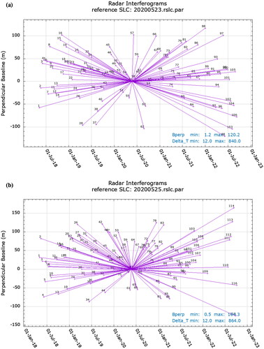
Since PS-InSAR technique selects one image as the reference (i.e. master image) to form all InSAR pairs, both image stacks were referenced to 2020/5/23 and 2020/5/25, respectively. Their spatial and temporal baseline plots are shown in Appendix B. Next, single-pixel differential interferometric phase techniques were employed to generate a co-registered SLC stack. Initially, two consecutive SLCs of the same epoch were examined and concatenated to form a single scene. Subsequently, the SLC datasets underwent radiometric calibration and processing to generate the Multi-look Intensity (MLI) mosaic and their geocoded products. Precise azimuth co-registration at sub-pixel scales is essential for TOPS interferometry to minimize phase jumps within bursts (Prats 2010). Therefore, iterative refinement procedures for burst overlap areas, utilizing intensity matching and the spectral diversity method (Scheiber and Moreira, 2000), were employed during co-registration. Azimuth de-ramping was estimated, followed by range oversampling, to accurately localize PS targets and eliminate the phase change effect caused by antenna pointing. The co-registered SLC stack was prepared as the initial step for PS-InSAR processing.

3.2.2. PS-InSAR processing

The PS-InSAR workflow then commenced with the identification of high-quality point target candidates characterized by low spectral phase diversity and minimal temporal backscatter variability (Werner et al. 2003). The spectral characteristics of point-like targets were initially extracted using spectral diversity based on the non-speckling effect in range and azimuth, yielding an initial point list with a spectral correlation threshold of 0.4 and a mean-to-sigma ratio of 1.0. Subsequently, the temporal variability method was employed with a minimum threshold of mean-to-standard deviation ratio (MSR) of 2.1 and an intensity minimum threshold relative to the spatial average of 0.5. This approach generated the second point list, considering the temporal variation of scatterers and average scene intensity. The final list of reliable points was then compiled for each data stack. SLC values and interferometric baseline information for final point candidates were estimated using orbit state vectors. Then, a precise and up-to-date 30 m resolution Copernicus DEM (COP-DEM, 2021) was employed for geocoding and local terrain height corrections.

Subsequently, a point data stack of differential interferograms was computed. Then, the spatial reference point was determined based on the quality of the points correlated to the phase standard deviation derived from the preliminary linear regression analysis. The interdependence of the interferometric phase with time and baseline was assessed through iterative 2D linear regression analysis. This process estimated point data stacks of linear deformation rates, height corrections, residual phase, unwrapped phase, and phase standard deviation as a refinement measure with each iteration, continuing until the minimum change in the parameters was observed. At each iteration level, spatial filtering of the differential interferogram was performed to remove phase noise and large-scale atmospheric phase trends. Four linear iterations were conducted to eliminate large-scale phase trends, estimate height corrections, and mitigate phase noise. This approach yielded final atmospheric phase signals and residual phases at each stage. At each level, residual phases underwent further analysis to detect any unwrapping phase ambiguities. These ambiguities were addressed at each iteration step through rewrapping, filtering, and spatial unwrapping procedures. Consequently, the final iteration produced deformation rate estimates, which were then extracted and converted into LOS displacement time series.

3.2.3. LOS InSAR decomposition and 2D displacement time series extraction

The LOS displacements from both orbits were decomposed to generate ENU displacement estimates. Initially, the LOS observations were geocoded using a similar DEM coverage. Subsequently, they were rasterized using least-squares interpolation to provide data in each grid of the geocoded products. To prevent extrapolation in areas lacking PS points, the interpolation distance was restricted to 50 m. However, due to SAR satellites’ near-polar trajectories, sensitivity in the north-south direction is very limited (Wright et al. 2004; Hu et al. 2014; Fuhrmann and Garthwaite, 2019). Therefore, the accurate retrieval of true 3D displacement was hindered by the exclusion of north-south deformation. Resultantly, the 2D deformation estimates were calculated using Equations 1(1) $$\left[A\right]\left[x\right]=\left[b\right]$$(1) and 2(2) $$\left[\begin{array}{c}-{\mathrm{\text{sin}}\theta }_{\mathit{\text{asc}}1}{\text{cosϕ}}_{\mathit{\text{asc}}1} {\mathrm{\text{cos}}\theta }_{\mathit{\text{asc}}1}\\ -{\mathrm{\text{sin}}\theta }_{\mathit{\text{asc}}2}{\text{cosϕ}}_{\mathit{\text{asc}}2} {\mathrm{\text{cos}}\theta }_{\mathit{\text{asc}}2}\\ ⋮\\ -{\mathrm{\text{sin}}\theta }_{\mathit{\text{des}}1}{\text{cosϕ}}_{\mathit{\text{des}}1} {\mathrm{\text{cos}}\theta }_{\mathit{\text{des}}1}\\ -{\mathrm{\text{sin}}\theta }_{\mathit{\text{des}}2}{\text{cosϕ}}_{\mathit{\text{des}}2} {\mathrm{\text{cos}}\theta }_{\mathit{\text{des}}2}\\ ⋮\end{array}\right]\left[\genfrac{}{}{0pt}{}{d_E}{d_U}\right]=\left[\begin{array}{c}{d}_{\mathit{\text{asc}}1}\\ d_{\mathit{\text{asc}}2}\\ ⋮\\ d_{\mathit{\text{des}}1}\\ d_{\mathit{\text{des}}2}\\ ⋮\end{array}\right]$$(2) , which involved constructing linear equations for each grid cell in the scene: (1) $$\left[A\right]\left[x\right]=\left[b\right]$$(1) (2) $$\left[\begin{array}{c}-{\mathrm{\text{sin}}\theta }_{\mathit{\text{asc}}1}{\text{cosϕ}}_{\mathit{\text{asc}}1} {\mathrm{\text{cos}}\theta }_{\mathit{\text{asc}}1}\\ -{\mathrm{\text{sin}}\theta }_{\mathit{\text{asc}}2}{\text{cosϕ}}_{\mathit{\text{asc}}2} {\mathrm{\text{cos}}\theta }_{\mathit{\text{asc}}2}\\ ⋮\\ -{\mathrm{\text{sin}}\theta }_{\mathit{\text{des}}1}{\text{cosϕ}}_{\mathit{\text{des}}1} {\mathrm{\text{cos}}\theta }_{\mathit{\text{des}}1}\\ -{\mathrm{\text{sin}}\theta }_{\mathit{\text{des}}2}{\text{cosϕ}}_{\mathit{\text{des}}2} {\mathrm{\text{cos}}\theta }_{\mathit{\text{des}}2}\\ ⋮\end{array}\right]\left[\genfrac{}{}{0pt}{}{d_E}{d_U}\right]=\left[\begin{array}{c}{d}_{\mathit{\text{asc}}1}\\ d_{\mathit{\text{asc}}2}\\ ⋮\\ d_{\mathit{\text{des}}1}\\ d_{\mathit{\text{des}}2}\\ ⋮\end{array}\right]$$(2) where rows in $\left[A\right]$ represent the unit look vector directing from radar to ground for each pixel on the map, expressed in ENU units and calculated from incidence angle $\theta$ and the satellite’s heading angle $\mathrm{\varphi }$ for each pixel, $\left[x\right]$ denotes the two unknown vectors, i.e. east-west and vertical displacement components, and $\left[b\right]$ represent the corresponding interpolated LOS estimates (known observation vectors) in ascending and descending orbits. Solving these equations yielded the displacement in the east-west and vertical dimensions. Further details on the methodology adopted can be found in Wegmüller et al. (2019) and Werner et al. (2017).

The procedure was then applied to both ascending and descending LOS datasets to estimate the 2D displacement, as mentioned below. Firstly, each layer was individually rasterized by iterating the procedure 106 times for ascending datasets and 116 times for descending datasets to estimate the LOS displacement at each time interval. Next, the closest (in time) pairs of ascending and descending LOS data were defined. As a result, 95 pairs were extracted from both datasets, and the remaining scenes from each orbit were discarded from further analysis. Due to the different acquisition times for both satellite orbits, there is always a time lag between each pair. Fortunately, the lag between the first ascending scene and the next descending scene in each pair was only two days. Therefore, over a 4.5-year period, it was assumed that the deformation within two days was negligible. The 2D displacement was then calculated for each pair using the steps outlined above. The acquisition time of ascending scenes in each pair constituted the observation time for 95 displacement estimates. These estimates were then stacked to produce east-west and vertical displacement time series and deformation rate maps for use in the spatio-temporal analysis.

4. Results

4.1. LOS deformation estimation

Firstly, the LOS deformation derived from ascending and descending Sentinel-1 datasets exhibits similar intrinsic properties, differing only in their LOS directions. Nevertheless, an abrupt transition from urban to mountainous terrain, predominantly covered with vegetation, is evident around the metropolitan area (Figure 1). These complex terrain environments could introduce unreliable deformation measurements, primarily due to inconsistent backscattering phase signals and phase-unwrapping issues (Liu et al. 2022). Furthermore, depending on the slope of mountainous terrains, notable discrepancies in LOS deformations between ascending and descending flight directions can occur due to variations in their projections and azimuth directions (Schaufler et al. 2018). Resultantly, LOS deformation measurements in mountainous areas were masked out to refine the analysis, focusing specifically on the Taipei basin area, as shown in Figure 1.

Secondly, LOS deformation results consistently demonstrate reliability in dense urban areas, effectively identifying distinct deformation patterns. As depicted in Figure 2(a,b), the LOS deformation maps obtained over the Taipei basin exhibit similar magnitudes, ranging from −18 to 18 mm/yr. Additionally, these results demonstrate consistent deformation of the order of −2 to −6 mm/yr across almost the entire basin. When contrasted with the maximum deformation of −18 mm/yr observed in certain zones, these deformation rates can be considered relatively stable. However, some uplifting signals were observed at the transition boundary between the mountains and urban areas, particularly around the top right corner. As mentioned previously, these zones mark abrupt changes in topographic conditions, which are highly likely to cause signal distortions due to changes in slope and terrain (Liu et al. 2022). Furthermore, complex terrain exacerbates the challenge of accurately retrieving topography-related phases, thereby introducing uncertainties in deformation analysis (Du et al. 2017; Xu et al. 2022). Consequently, these uplifting signals may be erroneous and therefore cannot be fully trusted. Fortunately, it is worth mentioning that these areas are situated beyond the downtown urban metropolitan area and do not significantly impact our analysis further.

Figure 2. Annual average line-of-sight (LOS) deformation in the study area from 2018 to 2022 in Sentinel-1 (a) ascending and (b) descending orbits. The brown text indicates the districts with distinct deformation patterns. The blue color indicates deformation away from the radar, while the red color indicates deformation towards the radar.

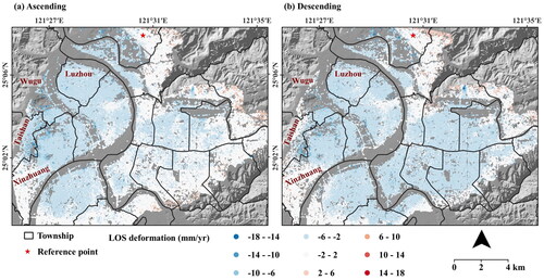
Lastly, distinct deformation patterns were detected in three districts, namely Wugu, Taishan and Xinzhuang, to the west of the study area. In these zones, the maximum and minimum deformation calculated from both the orbits were −18 and −6 mm/yr, respectively. Due to the lack of PS points at few locations, the deformation rate was not estimated. These are sub-urban and rural townships that are currently in development and have limited permanent targets for PS point generation. The deformation, calculated along the LOS direction, may include both vertical and horizontal components. Subsequently, the deformation was further analyzed and discussed in the following section.

4.2. 2D Vertical and east-west deformation estimates

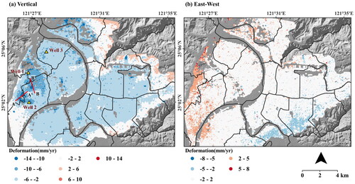
The InSAR-decomposed deformation rate maps were derived in accordance with the methodology outlined in Section 3.3. The vertical deformation map is depicted in Figure 3(a), illustrating variations in the average vertical deformation rate ranging from −14 to 14 mm/yr. Notably, this range exceeds the deformation observed in the east-west direction (Figure 3(b)), which ranges from −8 to 8 mm/yr. However, the vertical deformation signals unveil significant deformation within the metropolitan area. The entire study area was observed to be subsiding, with a magnitude ranging from −2 to −6 mm/yr. Additionally, the distinct deformation zones observed in the LOS direction can be clearly distinguished from InSAR-decomposed deformation estimates, primarily illustrating vertical deformation in three districts: Wugu, Taishan, and Xinzhuang. The subsidence calculated in these zones ranges from −6 to −14 mm/yr, with an average estimated to be approximately −1 cm/yr. Given the lesser deformation observed in the east-west direction, it was assumed that the study area is predominantly influenced by vertical deformation signals. Nonetheless, there exists horizontal deformation, albeit at a lower level of significance, which cannot be assumed negligible. As a result, the proposed method has demonstrated its significance in extracting the pure vertical displacement for further analysis.

Figure 3. LOS InSAR decomposed results showing (a) vertical and (b) east-west deformation. Blue color represents westward, or subsidence, while red depicts eastward, or upward deformation.

4.3. External validation using leveling datasets

For robust validation of InSAR-derived vertical deformation, ground measurement data from 104 first-order leveling stations was collected. Leveling data is collected annually or even every two years; thus, leveling data from 2016 to 2022 were acquired to ensure similar temporal coverage with InSAR, with at least three observations at each leveling station. The deformation rate at each station was then calculated using the linear least squares method. However, a few locations with only two observations were also considered to ensure full spatial coverage in the study area, and the deformation at these stations was calculated by evaluating the change in displacement over time. Based on the spatial distribution, almost all of the leveling stations are concentrated in relatively stable deformation zones (Figure 4(a)), as can also be inferred from the lower value range of InSAR vertical deformation, ranging from −6 to 3 mm/yr (Figure 4(b)). To facilitate a reasonable comparison of vertical deformation (U), PS points within a radius of 50 m centered around each leveling point were averaged to estimate the deformation at each location. The leveling and vertical deformation were then statistically compared, as depicted in Figure 4(b), with the results indicating good agreement. The correlation coefficient (r) was calculated to be 0.84, and the R-squared value was found to be 0.71. For error estimates, the root mean square error (RMSE) was calculated to be 2.81 mm/yr. However, it’s worth noting that the spatial reference location for both sets of observations differed, which could be attributed to variations in the elevation datum used in the spatio-temporal dimensions.

Figure 4. (a) Spatial distribution of the leveling stations overlapped on the InSAR-derived vertical deformation. (b) shows the statistical assessment between leveling and vertical deformation where the black line indicates the linear regression slope.

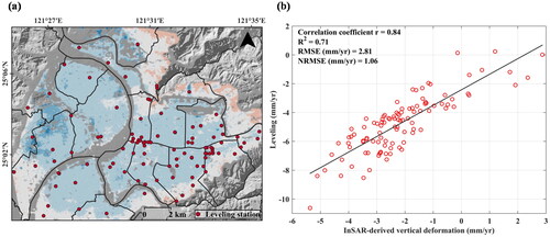
Resultantly, to mitigate the systematic offset caused by different reference locations in both datasets, the normalized root mean square error (NRMSE) was calculated. This adjustment allows for fairer comparisons to assess the accuracy of the datasets. NRMSE is widely used in several studies to normalize the effect due to diverse reference points (Kennedy-Asser et al. 2020; Tsai and Tseng, 2023). Mathematically, it is computed as: (3) $$\mathrm{\text{NRMSE}}=\sqrt{\frac{\sum _{i=1}^n{(L_i-U_i)}^2}{n}}$$(3) where $n$ is the total number of data points and $(L_i-U_i)$ is the normalized difference between leveling and vertical deformation, defined as follows: (4) $$L_i={\mathrm{ }l}_i–l_{\mathrm{\text{mean}}}$$(4) (5) $$U_i=u_i–u_{\mathrm{\text{mean}}}$$(5) where ${ l}_i$ and $u_i$ are the leveling and vertical deformation datasets. The $l_{\mathrm{\text{mean}}}$ and $u_{\mathrm{\text{mean}}}$ are the mean values of the leveling and vertical deformation datasets. The calculated NRMSE was 1.06 mm/yr, indicating good error estimates between the two observations. This was consistent with the magnitude of vertical deformation (U), which ranged between −2 and −6 mm/yr across almost the entire study area. This demonstrates the robustness of the InSAR results derived from the LOS InSAR decomposition analysis. However, as illustrated in Figure 4(b), there are systematic discrepancies between InSAR and leveling observations. These could primarily be attributed to the difference in the temporal resolution between InSAR multitemporal observations and leveling records. While InSAR data were acquired more frequently over the 4.5-year period, leveling measurements were much less frequent, averaging one per year or once every two years. This discrepancy in temporal resolution could limit the effectiveness of deformation estimation. As a result, compared to InSAR, leveling deformation is consistently overestimated. Secondly, it is often challenging to find InSAR observations that precisely coincide with the location of leveling benchmarks. This necessitates the use of buffer space to ensure an adequate number of PS pixels for analysis. Moreover, this approach may also sometimes be limited by the availability of PS measurement points, which can affect the accuracy of the comparison between InSAR and leveling data.

4.4. Spatio-temporal evolution of vertical displacement

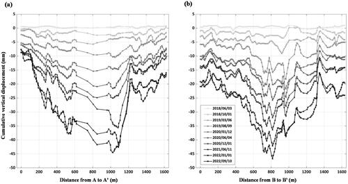
To further investigate the distinct deformation zones identified in Section 5.3, two linear profiles, A-A' and B-B', were considered in the subsidence zones, as depicted in Figure 3(a). PS points within 50 m of these profiles were then analyzed. As demonstrated in Figure 5(a,b), the variation of cumulative vertical displacement with distance from points A and B towards points A' and B' was evaluated at ten different time periods between 2018 and 2022. This analysis allowed for the observation of the subsidence evolution of each PS point in the spatio-temporal domain. According to the results, the vertical displacement increases gradually over time, forming a subsidence funnel at a depth of 600–1000 m, indicating significant deformation spots at the center. However, due to the undeveloped areas and few permanent structures along the A-A' profile, there are fewer PS points within this distance range, as seen in Figure 5(a). This limitation somehow restricted the accurate displacement estimation in this zone. Resultantly, all PS points within 1000 to 1100 m (Figure 5(a)) and 750 to 850 m (Figure 5(b)) were considered and averaged to quantify vertical deformation in these spots. The calculated results were −11.77 and −11.02 mm/yr, with high R-squared correlations of 0.98 and 0.99, respectively, signifying linear subsiding patterns over time.

Figure 5. Spatio-temporal evolution of vertical displacement at ten observation times between 2018 to 2022 for profiles (a) A–A’ and (b) B–B’.

4.5. Quantitative analysis of groundwater and vertical displacement

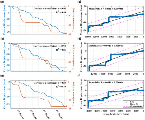
To delve deeper into the mechanism, groundwater observations close to the subsiding spots were examined. Groundwater well data situated in the vicinity of subsidence zones within the districts of Wugu, Xinzhuang, and Luzhou were accessible for analysis. At each location, both shallow and deep wells were present. For the analysis, groundwater data from the deeper wells were utilized, as they provide a more reliable indicator of groundwater level changes, particularly during periods of significant groundwater level drop. These data were recorded at a daily temporal resolution over a span of 4.5 years, capturing the fluctuations in groundwater levels on a daily basis. Given the extensive dataset available, statistical comparisons were performed to analyze and assess the differences between the two distinct observations. In theory, groundwater levels are subject to rapid fluctuations, which may not always correlate with surface deformation. This discrepancy arises because the surface typically does not respond immediately to changes in groundwater levels, even if the groundwater rebounds to a stable limit. This phenomenon was observed by Yang et al. (2019) in the Tianjin coastal area, where prolonged inelastic deformation persisted despite stable groundwater levels. Their study concluded that seasonal fluctuations in groundwater were the primary contributing factor to this phenomenon. Therefore, conducting a direct comparison to quantify the relationship between the two observations is complicated. Consequently, a new approach was adopted to effectively explore the relationship between groundwater observations and vertical displacement. Initially, the assumption was made that once the soil had been compressed, it would barely rebound. Following that, the groundwater level records were thoroughly examined to extract the time periods of decreasing groundwater levels in the entire time series with respect to immediate past observations. The remaining gaps were then filled by assuming constant groundwater levels at each day until the next decreasing groundwater level, and so on, to ensure continuous daily groundwater records. However, the vertical displacement time series were interpolated to produce daily observations over a 4.5-year period, and the average vertical displacement within 50 m of each well location was considered. Lastly, for each well location, the groundwater and InSAR-derived vertical displacement observations were statistically compared, as shown in Figure 6(a, c, and e). The trends at each location appear quite similar and consistent during the long monitoring period. Then, correlation analysis was performed, and the results indicated good consistency with correlation coefficients (r) of 0.92, 0.93, and 0.89, respectively, and R-squared values of 0.84, 0.86, and 0.79. To quantify the relationship between two observations, a hydraulic parameter, storativity (S), was estimated. In hydrogeology, storativity is the measure of the amount of water released from an aquifer per unit surface area and per unit decrease in hydraulic head. Several researchers (Chen et al., 2016; Liu et al. 2018) have utilized InSAR-derived vertical displacement to estimate storativity and assess the aquifer’s contribution to surface deformation. This was also calculated in this study: (6) $$S=\frac{\Delta U}{\Delta h}$$(6) where $\Delta U$ and $\Delta h$ shows the change in the vertical displacement and the groundwater level, respectively. To apply the above concept, daily observations in both cases were correlated using least squares regression in the temporal domain over a 4.5-year period, as shown in Figure 6(b, d, and f). Consequently, storativity and error estimates were computed as 0.0015 ± 0.000016, 0.0020 ± 0.000020, and 0.0011 ± 0.000014 at wells 1, 2, and 3 in the districts of Wugu, Xinzhuang, and Luzhou, respectively. High storativity values of 0.0020 and 0.0015 were observed at the locations of well 2 and well 1, respectively, which are situated within the distinct deformation zones. This illustrates that high storativity implies significant vertical displacement, demonstrating that fluctuations in groundwater levels are the primary cause of subsidence in Wugu, Taishan, and Xinzhuang.

Figure 6. Variation of vertical displacement and groundwater observations with time from 2018 to 2022 in (a) well 1, (c) well 2 and (e) well 3 in Wugu, Xinzhuang and Luzhou districts, respectively. The blue line shows vertical deformation, whereas orange represents groundwater observations. Linear regression analysis and quantification between groundwater observations and vertical displacement in (b) well 1, (d) well 2 and (f) well 3.

5. Discussions

5.1. Main findings of the present study

The findings of this study illustrate consistent results. As elaborated in Section 5.2, the LOS deformation estimates from both ascending and descending datasets exhibit consistent deformation patterns. Despite inherent uncertainties, statistical analyses indicate that errors in estimated deformation are less than 0.5 mm/yr, attributed to a 4.5-year time series and a large number of observations. Moreover, distinct areas of deformation are clearly discerned in both orbits, with deformation rates ranging from −18 to 18 mm/yr between 2018 and 2022. Additionally, significant vertical deformation was identified by examining signals in each directional component, revealing a maximum subsidence of −14 mm/yr (Figure 3(a)), with relatively minor horizontal deformation observed in the study area. Ground-based validation metrics further corroborate the credibility of the findings. These statistically validated linear subsidence trends underscore gradual deformation patterns averaging between −1 and −2 cm/yr over extended periods. A deeper understanding of the deformation mechanism elucidates groundwater fluctuations as the main cause of subsidence, based on the long-term temporal dynamics of vertical displacement and groundwater oscillations. A quantitative assessment, based on storativity values at three well locations in Wugu, Xinzhuang, and Luzhou districts, reveals that the Xinzhuang district is severely impacted by subsidence.

5.2. Comparison with other studies

Tung et al. (2016) previously investigated this study area employing X-band-derived time series InSAR and identified LOS deformation ranging from −15 to 15 mm/yr between 2011 and 2013, along with analogous distinct deformation zones. Another investigation conducted by a local institute (NCKU, 2023) utilized Sentinel-1 datasets with the SBAS-InSAR technique, disclosing no notable subsidence except for localized subsidence in the Wugu district, estimated at approximately −15 mm/yr from 2012 to 2020. Their analysis concluded that a substantial drop in groundwater levels in 2019 might be a potential driver of subsidence in these districts and cautioned against future subsidence due to ongoing development in the region. Despite disparities in observation periods and SAR sensors utilized, the outcomes of these studies are largely comparable. However, previous studies focused on single orbit datasets, in contrast to our study, which utilized dual orbit (ascending and descending) datasets for retrieving both vertical and east-west displacements. Additionally, it is evident that the LOS deformation noted in previous studies closely corresponds with the vertical deformation derived from the InSAR decomposition analysis in our study, suggesting notable vertical deformation with minimal horizontal displacement in the study region. Several researchers (Chen et al. 2014; Li et al. 2019) have studied the horizontal deformation field of Taiwan, clearly illustrating significantly lesser horizontal deformation influence in northern Taiwan compared to southern Taiwan, with observed rates around 4 to 5 mm/yr. These findings are consistent with the observations of this study.

5.3. Implication and explanation of findings

The deformation patterns were examined through aquifer parameter estimation, utilizing changes in deformation and groundwater at a daily temporal scale. Aquifer parameters related to storativity have been assessed concerning both elastic and inelastic aquifer deformation in various studies, with findings suggesting that inelastic deformation occurs when storativity exceeds 0.005 (Galloway et al. 1998; Liu et al. 2018). Our study indicates that the subsidence observed in these zones may result from elastic deformations, as indicated by a maximum cumulative value of 0.0020 in the Xinzhuang district. Previously, Tung et al. (2016) also evaluated the aquifer storativity parameter in the study area by correlating observations over sparse time periods. They identified higher values in the Wugu region, linking subsidence to the aquifer’s response in various geological formations. In contrast, based on our proposed methodology, the estimated storativity at the Wugu well location remained relatively consistent across two distinct observation periods. However, our research unveiled extensive deformation areas in the Xinzhuang district, corresponding to the highest storativity compared to the other two well locations. These findings suggest a significant expansion of deformation areas from the south of Wugu to the Xinzhuang district over a 12-year period, spanning from 2011 to 2022. These observations highlight the presence of persistent subsidence patterns within the study area.

5.4. Strengths and limitations

This study involves the extraction of pure vertical displacement through the decomposition of datasets from two orbits, aiming to investigate the spatio-temporal evolution of subsidence and its correlation with groundwater fluctuations. To derive the 2D displacement time series, careful consideration must be given to the LOS displacement layers for both ascending and descending datasets, focusing on the temporal gap between them. Unfortunately, the temporal misalignment of the two datasets, resulting from differing monitoring periods, poses a challenge. Secondly, due to technical issues, the inconsistency arises due to the unavailability of datasets from either satellite during some time periods. Depending on the time difference between the two observations, the reliability of statistics may be compromised by the assumption of no deformation during that interim period. Therefore, the primary concern should be to consider two displacement layers with minimum temporal gap for integration. Furthermore, aligning reference scenes and ensuring similar temporal coverage for the two LOS deformations is crucial. Lastly, for more reliable estimates, the large time series of InSAR datasets can be considered. Fortunately, our study effectively meets these criteria, as demonstrated by robust statistical validation using geodetic leveling datasets, ensuring the reliability of the results.

Additionally, PS point targets can be readily generated in densely populated metropolitan areas, with a decrease in density observed in rural or sparsely urban areas. However, while our study area features a significantly higher number of PS points, although there are comparatively fewer PS points in the rural areas within the distinct deformation zones. This limitation may hinder comprehensive deformation estimation. To address this issue, future research could incorporate a PS-DS approach to generate distributed scatterers in rural areas alongside permanent scatterers, potentially increasing the number of PS candidate points. Moreover, Global Navigation Satellite System (GNSS) datasets could be utilized to validate the ENU displacements derived from InSAR. Nevertheless, this study demonstrated significant vertical deformation and was robustly validated using first-order leveling datasets. However, the absence of suitable Continuously Operating Reference Stations (CORS) in the study area hampers the statistical verification of east-west deformation. Although true 3D deformation was not achievable in this study due to limited sensitivity to estimate north-south deformation, future work could incorporate multi-viewing observations using additional SAR sensors and GNSS datasets to retrieve the actual 3D displacements (Fuhrmann and Garthwaite, 2019). This could lead to a comprehensive understanding of deformation patterns in these areas.

Lastly, this study investigated long-term temporal dynamics between fluctuations in groundwater levels and land subsidence, primarily focusing on their correlation. Despite our efforts to explore these dynamics, their actual relationship remains uncertain, which underscores the need for further investigations. In the real-world scenario, the relationship between changes in groundwater levels and surface deformation is inherently complex, involving both linear and non-linear associations. This complexity presents challenges when attempting to understand these intricate relationships solely based on correlation coefficients (Janse et al. 2021). Additionally, observations by Burbey et al. (2006) and Ye et al. (2016) suggest that groundwater-induced deformations propagate in both vertical and horizontal dimensions, further complicating the challenge of estimating these deformations over large spatial-temporal coverage. Therefore, to further explore and quantify the relationship between groundwater dynamics and InSAR measurements, much more sophisticated techniques and analysis should be considered. Consequently, it is imperative to incorporate geophysical modeling utilizing 3D observations of groundwater flow and surface deformations to understand aquifer behavior. Bonì et al. (2020) developed geo-mechanical models based on groundwater flow observations and InSAR deformation measurements, concluding that the horizontal displacement field significantly characterizes aquifer properties. However, their study is limited by InSAR observations from a single orbit track. Their conclusions underscore the importance of 3D modeling to comprehend aquifer characteristics, integrating both horizontal and vertical deformation components. While these deformations have been previously computed, the ENU displacement time series has not been considered. In connection with this, our study demonstrates an alternative approach to accurately estimate InSAR-derived vertical and horizontal displacements, enabling a comprehensive understanding of temporal deformation dynamics. Additionally, more robust datasets, including historical land development patterns and hydrological datasets, could also be integrated into future work. Subsequently, to fully leverage the potential of multivariate datasets, structural equation modeling (SEM) can be employed to analyze intricate relationships between multiple factors. SEM is a robust statistical technique that involves integrating mathematical equations and digital analysis to extract hidden dynamic relationships, thus transforming traditional landscape performance factors into scientifically discernible constructs (Fornell & Larcker, 1981; Li et al. 2021). This approach has the potential to offer a more comprehensive understanding of Earth’s surface geodynamics. Resultantly, integrating geophysical modeling and the SEM technique into our future research endeavors could provide invaluable insights and enhance the scientific rigor of our conclusions.

6. Conclusion

To effectively quantify groundwater-related subsidence, this study explored extracting InSAR-derived east-west and vertical displacement time series from 2018 to 2022, aiming to understand the spatio-temporal evolution of deformation in the Taipei basin. The adopted methodology overcomes the constraints of previous studies by extensively utilizing both ascending and descending datasets to estimate individual displacement signals in the vertical and east-west directions. Results indicate that vertical deformation has a greater impact on the study area compared to horizontal deformation. Specifically, Wugu, Taishan, and Xinzhuang districts were identified as illustrating distinct subsidence patterns. Statistical validation with leveling datasets robustly affirmed the reliability of InSAR-derived vertical deformation. The results highlight the significant impact of groundwater fluctuations on subsidence in these districts, confirming purely elastic deformations based on calculated storativity values. Overall, the study reveals extended subsidence patterns averaging between −1 and −2 cm/yr across a broad region from Wugu to the Xinzhuang districts over a 12-year period from 2011 to 2022.

These findings demonstrate the robustness of the applied method in facilitating effective deformation estimations. However, the method’s reliance on closest displacement layers in ascending and descending tracks may not always be feasible, resulting in irregular temporal gaps in the derived east-west and vertical displacement time series. This could introduce uncertainties when assuming no deformation between corresponding displacement layers in each pair. Therefore, validation with secondary datasets is essential for additional accuracy statistics, as demonstrated in this study. In conclusion, the study provides a methodological framework for understanding deformation patterns in urban areas globally. The statistically validated findings support effective groundwater resource management in subsidence-prone zones.

Disclosure statement

No potential conflict of interest was reported by the authors.

Data availability statement

All data that support the findings of this research are available on request from the corresponding author.

Appendix

Appendix A.

The metadata of the employed Sentinel-1 datasets

Table

Flight direction	Ascending	Descending
Number of scenes	212	116
Path	69	105
Frame	74&79	510
Temporal coverage	2018/05/10-2022/09/10	2018/04/30-2022/10/06
Reference image date	2020/05/23	2020/05/25
Heading angle (°)	−12.47	192.47
Incidence angle (°)	42.21	36.28
Polarization	VV	VV

Appendix B.

The spatial and temporal baseline plots of SAR images stacks acquired in (a) ascending and (b) descending flight directions

References

- ASF. 2018. Copernicus Sentinel Data (2018, 2022). Retrieved from ASF DAAC [12/11/2021], processed by ESA. https://asf.alaska.edu/datasets/daac/sentinel-1/#
- Awasthi S, Jain K, Bhattacharjee S, Gupta V, Varade D, Singh H, Narayan AB, Budillon A. 2022. Analyzing urbanization induced groundwater stress and land deformation using time-series Sentinel-1 datasets applying PSInSAR approach. Sci Total Environ. 844:157103. doi: 10.1016/j.scitotenv.2022.157103.
- Bell JW, Amelung F, Ferretti A, Bianchi M, Novali F. 2008. Permanent scatterer InSAR reveals seasonal and long-term aquifer-system response to groundwater pumping and artificial recharge. Water Resour Res. 44(2). doi: 10.1029/2007WR006152.
- Berardino P, Fornaro G, Lanari R, Sansosti E. 2002. A new algorithm for surface deformation monitoring based on small baseline differential SAR interferograms. IEEE Trans Geosci Remote Sens. 40(11):2375–2383. doi: 10.1109/TGRS.2002.803792.
- Bonì R, Meisina C, Teatini P, Zucca F, Zoccarato C, Franceschini A, Ezquerro P, Béjar-Pizarro M, Fernández-Merodo JA, Guardiola-Albert C, et al. 2020. 3D groundwater flow and deformation modelling of Madrid aquifer. J Hydrol. 585:124773. doi: 10.1016/j.jhydrol.2020.124773.
- Burbey TJ, Warner SM, Blewitt G, Bell JW, Hill E. 2006. Three-dimensional deformation and strain induced by municipal pumping, part 1: analysis of field data. J Hydrol. 319(1-4):123–142. doi: 10.1016/j.jhydrol.2005.06.028.
- Castellazzi P, Garfias J, Martel R. 2021. Assessing the efficiency of mitigation measures to reduce groundwater depletion and related land subsidence in Querétaro (Central Mexico) from decadal InSAR observations. Int J Appl Earth Obs. Geoinf. 105:102632. doi: 10.1016/j.jag.2021.102632.
- Chen J,Knight R,Zebker HA,Schreüder WA. 2016. Confined aquifer head measurements and storage properties in the San Luis Valley, Colorado, from spaceborne InSAR observations. Water Resour Res. 52(5):3623–3636. doi: 10.1002/2015WR018466.
- Chen B, Gong H, Chen Y, Lei K, Zhou C, Si Y, Li X, Pan Y, Gao M. 2021. Investigating land subsidence and its causes along Beijing high-speed railway using multi-platform InSAR and a maximum entropy model. Int J. Appl Earth Obs Geoinf. 96:102284. doi: 10.1016/j.jag.2020.102284.
- Chen J, Knight R, Zebker HA. 2017. The temporal and spatial variability of the confined aquifer head and storage properties in the San Luis Valley, Colorado Inferred from multiple InSAR missions. Water Resour Res. 53(11):9708–9720. doi: 10.1002/2017WR020881.
- Chen KH, Hwang C, Tanaka Y, Chang PY. 2023. Gravity estimation of groundwater mass balance of sandy aquifers in the land subsidence-hit region of Yunlin County, Taiwan. Eng Geol. 315:107021. doi: 10.1016/j.enggeo.2023.107021.
- Chen SK, Chan YC, Hu JC, Kuo LC. 2014. Current crustal deformation at the junction of collision to subduction around the Hualien area, Taiwan. Tectonophysics. 617:58–78. doi: 10.1016/j.tecto.2014.01.014.
- Chia Y-P, Chang M-H, Liu W-I, Lai T-C. 1999. Hydrogeologic characterization of Taipei Basin (in Chinese with English abstract). Cent Geol Surv Spec Publ. 11:393–406.
- Cigna F, Tapete D. 2021. Present-day land subsidence rates, surface faulting hazard and risk in Mexico City with 2014–2020 Sentinel-1 IW InSAR. Remote Sens Environ. 253:112161. doi: 10.1016/j.rse.2020.112161.
- COP-DEM. 2021. Copernicus digital elevation model. European Space Agency. doi: 10.5270/ESA-c5d3d65.
- De Zan F, Monti Guarnieri A. 2006. TOPSAR: terrain observation by progressive scans. IEEE Trans Geosci Remote Sensing. 44(9):2352–2360. doi: 10.1109/TGRS.2006.873853.
- Dixon T, Amelung F, Ferretti A, Novali F, Rocca F, Dokka R, Sella G, Kim S, Wdowinski S, Whitman D. 2006. Subsidence and flooding in New Orleans. Nature. 441(7093):587–588. doi: 10.1038/441587a.
- Dong J, Lai S, Wang N, Wang Y, Zhang L, Liao M. 2021. Multi-scale deformation monitoring with Sentinel-1 InSAR analyses along the Middle Route of the South-North Water Diversion Project in China. Int J Appl Earth Obs Geoinf. 100:102324. doi: 10.1016/j.jag.2021.102324.
- Du Y, Zhang L, Feng G, Lu Z, Sun Q. 2017. On the accuracy of topographic residuals retrieved by MTInSAR. IEEE Trans Geosci Remote Sens. 55(2):1053–1065. doi: 10.1109/TGRS.2016.2618942.
- Eriksen HØ, Lauknes TR, Larsen Y, Corner GD, Bergh SG, Dehls J, Kierulf HP. 2017. Visualizing and interpreting surface displacement patterns on unstable slopes using multi-geometry satellite SAR interferometry (2D InSAR). Remote Sens Environ. 191:297–312. doi: 10.1016/j.rse.2016.12.024.
- Ferretti A, Prati C, Rocca F. 2001. Permanent scatterers in SAR interferometry. IEEE Trans Geosci Remote Sensing. 39(1):8–20. doi: 10.1109/36.898661.
- Fornell C, Larcker DF. 1981. Evaluating structural equation models with unobservable variables and measurement error. J Mark Res. 18(1):39–50. doi: 10.2307/3151312.
- Fuhrmann T, Garthwaite MC. 2019. Resolving three-dimensional surface motion with InSAR: constraints from multi-geometry data fusion. Remote Sens. 11(3):241. doi: 10.3390/rs11030241.
- Galloway DL, Burbey TJ. 2011. Review: regional land subsidence accompanying groundwater extraction. Hydrogeol J. 19(8):1459–1486. doi: 10.1007/s10040-011-0775-5.
- Galloway DL, Hudnut KW, Ingebritsen SE, Phillips SP, Peltzer G, Rogez F, Rosen PA. 1998. Detection of aquifer system compaction and land subsidence using interferometric synthetic aperture radar, Antelope Valley, Mojave Desert, California. Water Resour. Res. 34(10):2573–2585. doi: 10.1029/98WR01285.
- Garg S, Motagh M, Indu J, Karanam V. 2022. Tracking hidden crisis in India’s capital from space: implications of unsustainable groundwater use. Sci Rep. 12(1):651. doi: 10.1038/s41598-021-04193-9.
- Herrera-García G, Ezquerro P, Tomás R, Béjar-Pizarro M, López-Vinielles J, Rossi M, Mateos RM, Carreón-Freyre D, Lambert J, Teatini P, et al. 2021. Mapping the global threat of land subsidence. Science. 371(6524):34–36. doi: 10.1126/science.abb8549.
- Hu J, Li ZW, Ding XL, Zhu JJ, Zhang L, Sun Q. 2014. Resolving three-dimensional surface displacements from InSAR measurements: a review. Earth-Sci Rev. 133:1–17. doi: 10.1016/j.earscirev.2014.02.005.
- Hu J, Motagh M, Guo J, Haghighi MH, Li T, Qin F, Wu W. 2022. Inferring subsidence characteristics in Wuhan (China) through multitemporal InSAR and hydrogeological analysis. Eng Geol. 297:106530. doi: 10.1016/j.enggeo.2022.106530.
- Janse RJ, Hoekstra T, Jager KJ, Zoccali C, Tripepi G, Dekker FW, van Diepen M. 2021. Conducting correlation analysis: important limitations and pitfalls. Clin Kidney J. 14(11):2332–2337. doi: 10.1093/ckj/sfab085.
- Kennedy-Asser AT, Lunt DJ, Valdes PJ, Ladant J-B, Frieling J, Lauretano V. 2020. Changes in the high-latitude Southern Hemisphere through the Eocene–Oligocene transition: a model–data comparison. Clim Past. 16(2):555–573. doi: 10.5194/cp-16-555-2020.
- Kim J, Lin S-Y, Singh T, Singh RP. 2023. InSAR time series analysis to evaluate subsidence risk of monumental Chandigarh City (India) and surroundings. IEEE Trans Geosci Remote Sensing. 61:1–15. doi: 10.1109/TGRS.2023.3305863.
- Leake SA. 2016. USGS: Land subsidence from ground-water pumping.
- Li CK, Ching KE, Chen KH. 2019. The ongoing modernization of the Taiwan semi-dynamic datum based on the surface horizontal deformation model using GNSS data from 2000 to 2016. J Geod. 93(9):1543–1558. doi: 10.1007/s00190-019-01267-5.
- Li M, Zhang X, Bai Z, Xie H, Chen B. 2022. Land subsidence in Qingdao, China, from 2017 to 2020 based on PS-InSAR. IJERPH. 19(8):4913. doi: 10.3390/ijerph19084913.
- Li Z, Han X, Lin X, Lu X. 2021. Quantitative analysis of landscape efficacy based on structural equation modelling: empirical evidence from new Chinese style commercial streets. Alex. Eng. J. 60(1):261–271. doi: 10.1016/j.aej.2020.08.005.
- Liu Y, Zhao C, Zhang Q, Yang C, Zhang J. 2018. Land Subsidence in Taiyuan, China, monitored by InSAR technique with multisensor SAR datasets from 1992 to 2015. IEEE J Sel Top Appl Earth Observations Remote Sensing. 11(5):1509–1519. doi: 10.1109/JSTARS.2018.2802702.
- Liu Z, Qiu H, Zhu Y, Liu Y, Yang D, Ma S, Zhang J, Wang Y, Wang L, Tang B. 2022. Efficient identification and monitoring of landslides by time-series InSAR combining single- and multi-look phases. Remote Sens. 14(4):1026. doi: 10.3390/rs14041026.
- Metzger LF, Ikehara ME, Howle JF. 2001. Vertical-deformation, water-level, microgravity, geodetic, water-chemistry, and flow-rate data collected during injection, storage, and recovery tests at Lancaster, Antelope Valley, California. U.S. Geological Survey Publication. September 1995 through September 1998, Open-File Report. doi: 10.3133/ofr01414.
- Marotti L, Wollstadt S, Scheiber R. 2023. Overview of Taipei subsidence. http://www.lsprc.ncku.edu.tw/en/trend.php?action=view&id=14
- Prats P. 2010. Investigations on TOPS interferometry with TerraSAR-X. In: 2010 Int. Geosci. Remote Sens. Symp. pp. 2629–2632. doi: 10.1109/IGARSS.2010.5650037.
- Ramirez RA, Lee GJ, Choi SK, Kwon TH, Kim YC, Ryu HH, Kim S, Bae B, Hyun C. 2022. Monitoring of construction-induced urban ground deformations using Sentinel-1 PS-InSAR: the case study of tunneling in Dangjin, Korea. Int J Appl Earth Obs Geoinf. 108:102721. doi: 10.1016/j.jag.2022.102721.
- Rezaei A, Mousavi Z. 2019. Characterization of land deformation, hydraulic head, and aquifer properties of the Gorgan confined aquifer, Iran, from InSAR observations. J Hydrol. 579:124196. doi: 10.1016/j.jhydrol.2019.124196.
- Riley FS. 1969. Analysis of borehole extensometer data from central California. Int Assoc Sci Hydrol Publ. 89:423–431.
- Rucci A, Ferretti A, Monti Guarnieri A, Rocca F. 2012. Sentinel 1 SAR interferometry applications: the outlook for sub millimeter measurements. Remote Sens. Environ. 120:156–163. doi: 10.1016/j.rse.2011.09.030.
- Schaufler S, Bauer-Marschallinger B, Hochstöger S, Wagner W. 2018. Modelling and correcting azimuthal anisotropy in Sentinel-1 backscatter data. Remote Sens Lett. 9(8):799–808. doi: 10.1080/2150704X.2018.1480071.
- Scheiber R, Moreira A. 2000. Coregistration of interferometric SAR images using spectral diversity. IEEE Trans Geosci Remote Sens. 38(5):2179–2191. doi: 10.1109/36.868876.
- Solano-Rojas D, Wdowinski S, Cabral-Cano E, Osmanoğlu B. 2020. Detecting differential ground displacements of civil structures in fast-subsiding metropolises with interferometric SAR and band-pass filtering. Sci Rep. 10(1):15460. doi: 10.1038/s41598-020-72293-z.
- Teng LS, Lee CT, Peng C-H, Chen W-F, Chu C-J. 2001. Origin and geological evolution of the Taipei Basin. Northern Taiwan West Pac Earth Sci. 1:115–142.
- Teng LS, Yuan PB, Chen P-Y, Peng C-H, Lai T-C, Fei L-Y, Liu H-C. 1999. Lithostratigraphy of Taipei Basin deposits (in Chinese with English abstract). Cent Geol Surv Spec Publ. 11:41–66.
- Terzaghi K. 1925. Principles of soil mechanics, IV—Settlement and consolidation of clay. Eng News-Record. IV:874–878.
- Torres R, Snoeij P, Geudtner D, Bibby D, Davidson M, Attema E, Potin P, Rommen B, Floury N, Brown M, et al. 2012. GMES Sentinel-1 mission. Remote Sens Environ. 120:9–24. doi: 10.1016/j.rse.2011.05.028.
- Tsai Y-LS, Tseng K-H. 2023. Monitoring multidecadal coastline change and reconstructing tidal flat topography. Int J Appl Earth Obs Geoinf. 118:103260. doi: 10.1016/j.jag.2023.103260.
- Tung H, Chen HY, Hu JC, Ching KE, Chen H, Yang KH. 2016. Transient deformation induced by groundwater change in Taipei metropolitan area revealed by high resolution X-band SAR interferometry. Tectonophysics. 692:265–277. doi: 10.1016/j.tecto.2016.03.030.
- Wegmüller U, Werner C, Magnard C, Manconi A. 2019. Co-seismic displacement vector retrieval for the Iran-Iraq Earthquake using Sentinel-1. Gümligen, Switzerland: GAMMA Remote Sensing. http://www.gamma-rs.ch
- Werner C, Baker B, Cassotto R, Magnard C, Wegmüller U, Fahnestock M. 2017. Measurement of fault creep using multi-aspect terrestrial radar interferometry at Coyote Dam. In 2017 IEEE Int. Geosci. Remote Sens. Symp. (IGARSS), pp. 949–952. doi: 10.1109/IGARSS.2017.8127110.
- Werner C, Wegmüller U, Strozzi T, Wiesmann A. 2000. GAMMA SAR and interferometric processing software. European Space Agency, (Special Publication) ESA SP, 211–219.
- Werner C, Wegmuller U, Strozzi T, Wiesmann A. 2003. Interferometric point target analysis for deformation mapping, in. IGARSS 2003. 2003 IEEE Int. Geosci. Remote Sens. Symp. Proceedings (IEEE Cat. No.03CH37477). vol.7, pp. 4362–4364. doi: 10.1109/IGARSS.2003.1295516.
- Wright TJ, Parsons BE, Lu Z. 2004. Toward mapping surface deformation in three dimensions using InSAR. Geophys Res Lett. 31(1) doi: 10.1029/2003GL018827.
- Xu H, Chen F, Zhou W, Wang C. 2022. Reducing the residual topography phase for the robust landscape deformation monitoring of architectural heritage sites in mountain areas: the pseudo-combination SBAS method. Remote Sens. 14(5):1178. doi: 10.3390/rs14051178.
- Yang J, Cao G, Han D, Yuan H, Hu Y, Shi P, Chen Y. 2019. Deformation of the aquifer system under groundwater level fluctuations and its implication for land subsidence control in the Tianjin coastal region. Environ Monit Assess. 191(3):162. doi: 10.1007/s10661-019-7296-4.
- Ye S, Luo Y, Wu J, Yan X, Wang H, Jiao X, Teatini P. 2016. Three-dimensional numerical modeling of land subsidence in Shanghai, China. Hydrogeol J. 24(3):695–709. doi: 10.1007/s10040-016-1382-2.
- Zebker HA, Rosen PA, Hensley S. 1997. Atmospheric effects in interferometric synthetic aperture radar surface deformation and topographic maps. J Geophys Res. 102(B4):7547–7563. doi: 10.1029/96JB03804.
- Zebker HA, Villasenor J. 1992. Decorrelation in interferometric radar echoes. IEEE Trans Geosci Remote Sensing. 30(5):950–959. doi: 10.1109/36.175330.
- Zhang Y, Gong H, Gu Z, Wang R, Li X, Zhao W. 2014. Characterization of land subsidence induced by groundwater withdrawals in the plain of Beijing city, China. Hydrogeol J. 22(2):397–409. doi: 10.1007/s10040-013-1069-x.