Reconstructing the 1968 River Chew flash flood: merging a HEC-RAS 2D hydraulic modelling approach with historical evidence

Abstract

The devastating 1968 flash flood in the River Chew, South-West of England, serves as a stark reminder of the unpredictable nature of such natural disasters and highlights the importance of natural hazard assessments. The uncertain and often incomplete historical data, and the limited field measurements at the time hindered our understanding of this event. By integrating historical evidence, including technical reports, newspapers, literature, and eyewitness accounts, with advanced hydraulic modelling (HEC-RAS 2D), this study reconstructs the 1968 flash flood. A sensitivity analysis of the computational methodologies in HEC-RAS, examining various governing equations and numerical methods, introduces an additional dimension to this research. The results verify a maximum flow rate of 165 m³/s at the Compton Dando hydrometric station, marking a 65% increase from the previous official estimate. This update aligns with over 90% of the historical flood marks observed. Findings suggest recalibrating hydrological models, revising risk assessments, and updating flood frequency analyses in the study area. This novel framework confronts the challenges of uncertain and incomplete historical records through a reverse engineering methodology to reconstruct missing peak discharges. The study also presents a new methodological blueprint that can be replicated for reconstructing historical flash flood events in various regions.

Keywords:

• HEC-RAS 2D
• reconstructing historical floods
• flash flood
• hydraulic modelling
• great flood of 1968

1. Introduction

Hydraulic reconstruction of historical flood events is often conducted to increase the understanding of the long-term exposure of riparian communities to the risk of flooding (Benito et al. 2023). Assessments of long-term flood risk are performed using flood frequency analysis techniques which commonly rely on the statistical analysis of peak flow series in the form of annual maximum series (Stedinger et al. 1993). It is therefore important that reconstruction events include an estimate of both the timing and magnitude of the peak flow. This is particularly true for catchments prone to flash floods resulting in large year-to-year variations in maximum flood levels (Mehta and Kumar 2022b).

In the scientific literature attempts to reconstruct historical floods have primarily focused on large rivers and major towns and cities with a long history and often a rich archive of documentary evidence such as newspaper articles, flood marks on historical buildings and bridges, photos, paintings and eyewitness accounts (e.g. Benito et al. 2004; Kjeldsen et al. 2014). Examples of such studies conducted to increase the reliability of design flood estimation are listed in Table 1. The listed studies apply a range of hydraulic modelling approaches to convert historical estimates of maximum water depth into the equivalent flood flow, ranging from simple applications of Manning’s equation and rating curves to application of modern advanced coupled 1D and 2D modelling systems. There is a noticeable dearth of research focused on the hydraulic reconstruction of less documented, yet impactful, flash flood events. This gap in the literature suggests an urgent need for studies that leverage advanced hydraulic modelling to develop new insight into the historical events that have shaped landscapes and communities. Such research would not only shed light on individual events with greater clarity but also demonstrate the potential of hydraulic modelling as a tool for enhancing the credibility of contemporary and future flood risk assessments. Addressing this gap is imperative for advancing the field of flood risk management and for developing a more accurate comprehension of flood dynamics across time and space.

Table 1. Examples of published case studies reconstructing historical flood events.

Country	River	City /Town	Year	Reference
Germany	Elbe	Dresden	1501–1929	Bartl et al. (2009)
Czechia	Vltava	Prague	1481–1825	Elleder et al. (2013)
Slovakia	Danube	Bratislava	1501, 1682, and 1787	Pekárová et al. (2013)
United Kingdom	Bristol Avon	Bath	1823–1969	Stamataki and Kjeldsen (2021)
Spain/Portugal	Guadiana	Badajoz	1876	González-Cao et al. (2021)
Germany	Rhine	Cologne	1374	Ngo et al. (2023)
Italy	Tiber	Rome	1870	Mancini et al. (2022)

While understanding the flood risk of the large river systems listed in Table 1 is important, it is also vital to emphasize the need to understand flood risk at a more local scale and smaller river systems; in particular the risk faced by communities living next to rivers prone to flash floods. Hydraulic reconstruction of past events in such locations is often made more difficult by the lack of easily available documentary evidence (Mehta et al. 2022a). However, there is a growing interest in the subject of reconstructing flash flood events in data-sparse regions as evidenced by, for example, Thomas et al. (2023) and Ngo et al. (2023).

Reconstruction of local flash flood events is complicated by the potentially large impact of singular features on the hydraulic characteristics of the event; both spatially and temporally. For example, Thomas et al. (2023) highlighted the importance of debris blocking as a feature not easily incorporated. Stamataki and Kjeldsen (2021) discussed the importance of a particular (and no longer existing) arch-bridge in controlling upstream water levels reached during past events.

It is recognized that the reliability of the reconstructed flood events should be considered as input to a flood frequency analysis. Prosdocimi (2018) discussed the importance of knowing the timing of the peaks and the beginning of the historical record. Lucas et al. (2023) considered the uncertainty on the magnitude of historical events and concluded that the potentially large uncertainty of reconstructed flood events limits their utility in reducing the overall uncertainty of design flood estimates derived from long data series yet can be useful as supplementary data with short data series available. Thus, it is key to understand the trade-off between the uncertainty of the reconstructed events and the general availability of long-term flood data.

It is clear that accurate estimation of the magnitude of past flood events is key to providing credible prediction of current and future flood risk. Therefore, it is important to fully understand how best to combine often uncertain and incomplete historical flood evidence with advanced modern numerical hydraulic models to achieve this. This is an important gap in the existing scientific literature and this study introduces a new methodology that integrates historical flood data with advanced hydraulic modelling (HEC-RAS 2D) in an attempt to address the two key themes previously outlined: reconstructing a significant flash flood event along a river that inflicted considerable damage on local communities, and the imperative to grasp the uncertainties inherent in this reconstruction process. Central to the methodology is the application of a reverse engineering approach, which enables systematic deduction of the hydrological conditions prevailing during the July 1968 event by working backwards from the known impacts and historical evidence. This reverse engineering process is pivotal in navigating the challenges posed by relying on disparate and uncertain historical data. The study demonstrates that reconstruction is feasible using the advanced hydraulic model HEC-RAS 2D, while also highlighting the challenges posed by uncertain historical evidence.

2. Case study and data collection

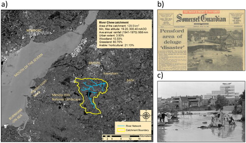
This study focuses on the reconstruction of a particular major flash flood event that occurred on the River Chew in the southwest of England on 10 July 1968 (Figure 1). The 1968 event was chosen particularly due to the high impact of this flash flood on the region, resulting in eight casualties (https://www.bristolpost.co.uk/news) and causing extensive destruction. Another major reason for selecting this event is the incomplete hydrograph due to the limitations of measuring devices at the time. This hydrograph, which serves as an indicator of the flood’s significance, can lead to an informed hazard assessment associated with flash floods in the area. The availability of official measured flood marks, which play a key role in the reconstruction of historical flash floods, was another reason to choose this case. The event unfolded as a result of unprecedented rainfall, with amounts ranging between 173 mm and 175 mm recorded within a span of 7 h to 9 h. The significance of the event is underscored by its documentation in key sources such as the UK Meteorological Office’s British Rainfall (BR)_1968, Salter (1968), and Hand et al. (2004), highlighting that the rainfall volume represented about 20% of the region’s average annual rainfall of 935 mm from 1916 to 1970 (BR_1969 and BR_1970).

Figure 1. (a) River Chew catchment and associated river network within the regional map. (b) Somerset Guardian newspaper from 12 July 1968, detailing the flood destruction and its impact on pensford, provided by the Pensford local history group. (c) Playground inundated by the flood in Keynsham’s town Centre, source: https://www.bristolpost.co.uk/news/bristol-news/gallery/great-flood-1968-bristol-1765201.

2.1. Hydrometric data

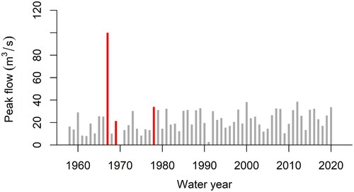
The Environment Agency and its predecessors have been operating a flow gauging station on the River Chew near the village of Compton Dando since 1958, recording water levels at 15-minute intervals and converting these into flow via rating curves. A quality-controlled annual maximum series of peak flow is available from the National River Flow Archive (NRFA) and is shown in Figure 2. According to this dataset, the magnitude of the 1968 flood was exactly 100 m³/s, which is a revised estimate and down from the initial value of 226.48 m³/s reported in the Flood Studies Report (NERC, 1975). An internal note from an author-unbeknown within the NRFA suggests that the initial estimate of 226 m³/s (8000 ft³/s) is ‘almost certainly estimated wrongly’. As very large events will have a substantial influence on estimates of design floods in the wider region, it is important that the magnitude of this event is established with more credibility than is currently the case.

Figure 2. Annual maximum series of peak flow (m³/s), from the River Chew at Compton Dando between 1958 and 2020 (water year). Red bars, indicate events that occurred between April and September (summer events).

2.2. Historical information

The July 1968 event caused extensive damage to the local community. The village of Pensford was particularly badly damaged, including the destruction of a major road bridge (A37), several houses and widespread inundation. Additional documentary evidence of the magnitude of the 1968 flood was collected from the area via a literature review, a series of site visits by the project team, and a community workshop organized on 30 September 2023 in collaboration with the Pensford Local History Group and attended by about 40 members of the local community. During the workshop, attendees were encouraged to share their memories, photographs, letters etc. related to the flood event (https://www.docuflood.uk/workshops). The data collection focused on evidence which could be translated into estimates of water levels with reasonable accuracy as to timing, thereby allowing a direct comparison between evidence and output from the hydraulic simulations. A summary of the collected evidence is shown in Table 2.

Table 2. Summary of documentary evidence for the July 1968 Pensford flood, including official flood marks and archive photos taken immediately after the event.

Name	Photo	Description	Name	Photo	Description
Floodmark A		Location: Coombe House, Church Street Type: Official flood mark Reference: Photograph by Ioanna Stamataki, 2021 Coordinate: 51.371288, −2.548529 Translation: 2.370 m above street level Timestep: At Peak Uncertainty: Brick did not exist in the correct size	Flood mark D		Location: The Rising Sun Pub Type: Indicative level Reference: Photograph by Ioanna Stamataki, 2023 Coordinate: 51.371396, −2.550037 Translation: ∼1.65–1.75 m above street level Timestep: At Peak Uncertainty: N/A
Floodmark B		Location: Church Wall, Church Street Type: Official flood mark Reference: Photograph by Ioanna Stamataki, 2021 Coordinate: 51.371218, −2.549393 Translation: 2.341 m above street level Timestep: At Peak Uncertainty: N/A	Flood mark E		Location: Coombe House, Church Street Type: Indicative level Reference: Pensford Local History Group’s Robert Bailey Collection (RBC 0068) Coordinate: 51.371162, −2.548406 Translation: ∼1.8–2.1 m above street level Timestep: At Peak Uncertainty: N/A
Floodmark C		Location: Mill Corner Garage, Church Street Type: Official flood mark Reference: Photograph by Ioanna Stamataki, 2021 Coordinate: 51.371488, −2.550173 Translation: 2.051 m above street level Timestep: At Peak Uncertainty: N/A	Flood mark F		Location: Floodmark at Coombe House, Church Street Type: Indicative level Reference: Pensford Local History Group’s Robert Bailey Collection (RBC 0078) Coordinate: 51.371288, −2.548529 Translation: ∼2.10–2.20 m above street level Timestep: At Peak Uncertainty: N/A

2.3. Digital elevation model and landcover map

To develop a Digital Elevation Model (DEM) for use in the hydrology and hydraulic models, a 1 × 1 m resolution composite Digital Terrain Model (DTM)-2023 was merged with a 1 × 1 m resolution composite Digital Surface Model (DSM)-2023 employing the ArcMap 10.8.2. The aim was to include buildings from the DSM while removing trees from the final DEM. This technique allows for the consideration of buildings’ impact while mitigating the influence of trees, as Cahyono and Hak (2023) indicated that trees could negatively affect and often lead to inaccurate predictions in hydraulic models reliant on terrain data. It is important to note in our modelling, we simulate buildings as impermeable objects, a simplification that, while generally effective, does not account for the complexities of flood dynamics where buildings might also be subject to flooding, albeit at a slower rate. This limitation stems from the fact that our DEM does not provide data on the potential permeability of these structures. Another reason for adopting the merged model was to accurately represent the Pensford Bridge in the 1968 reconstruction, which had been destroyed in the flood. The DTM and DSM, both sourced from the UK Environmental Agency, are LiDAR-derived datasets.

A landcover Map produced by the UK Centre for Ecology and Hydrology (UKCEH, 2021; Marston et al. 2022) was used to parameterize the hydrological and hydraulic models. This map was scaled at 1:250,000 and features a pixel resolution ranging between 10 and 25 meters.

3. Hydrology and hydraulic modelling

For hydrological and hydraulic simulation of the 1968 flood event, the HEC-HMS and the unsteady flow module of HEC-RAS 2D, version 6.4.1, developed by USACE, were chosen, though other two-dimensional Unsteady model could potentially have been used, e.g. FLOW (TUFLOW), SOBEK, LISFLOOD-FP, TELEMAC 2D, and Flow-2D. The selection of HEC-RAS was supported by studies such as Brunner (2018), which evaluated HEC-RAS 2D’s capability against benchmark tests from the UK’s Joint Department for Environment Food and Rural Affairs (Defra) and Environment Agency, demonstrating HEC-RAS's superior performance compared to other tested models (i.e. TUFLOW, MIKE FLOOD, SOBEK). Moreover, our choice of HEC-RAS for this research is reinforced by its proven accuracy in modelling critical flood scenarios, as evidenced by its use in predicting dam bursts in the Neelum River region (Niaz et al. 2023), flood overtopping in the Mengzong Gully (Huo et al. 2016). Furthermore, Ghimire et al. (2022) study indicated that, while the coupled 1D/2D model were not significantly outperformed the 1D model, the 2D model itself showed enhanced performance over both the coupled and 1D models in statistical analysis and visual comparison of observed stage and flow data.

3.1. Hydrology model (HEC-HMS)

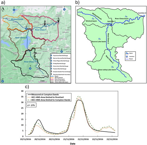
Acknowledging the scarcity of hydrometric stations upstream of our area of interest, the HEC-HMS was employed as the rainfall-runoff model to generate the input hydrograph for the hydraulic model. Given that this study predominantly concentrates on reconstructing the 1968 flood through hydraulic modelling, here we briefly outline the hydrology study’s overview, including the setup and calibration procedures of the hydrology model. The Chew catchment upstream of Pensford includes three main reaches of River Chew and a reach of Winford Brook. Consequently, this area was split into to four sub-catchments (Figure 3a). During the calibration process, the downstream area of the River Chew catchment was confined to the location of the Compton Dando hydrometric station, enabling a direct comparison between simulations and measurements. However, after calibration, the catchment was extended to align with the upstream boundary specified for the hydraulic model, which necessitates the input hydrograph (Location B) (Figure 3a). The crafted DEM was used to determine the necessary parameters for the HEC-HMS model, i.e. the area and slope of basins and reaches, and the length of the reaches.

Figure 3. (a) Boundaries of four basins with their corresponding Rivers, and location of rainfall gauges. (b) Overview of HEC-HMS setup (c) Comparison of observed flow rates at Compton Dando against HEC-HMS simulations for the same location, and generated hydrograph by calibrated HEC-HMS where the area is confined to Pensford (all graphs relating to the event of 20^th to 23^rd november 2016). $\epsilon$ is the relative absolute error (%) between the observation and simulation at Compton Dando as defined in Equation-1.

The Soil Conservation Service (SCS)-Curve Number (CN) method was selected to account for the hydrological losses supported by numerous studies such as the recent work of Yang et al. (2023). This model requires the CN, time of concentration, and lag time of basins as inputs. The CN of each sub-catchment was determined from a landcover map in conjunction with the Hydrology of Soil Types (HOST) dataset. This dataset groups soils into 29 classes, focusing on their ability to transmit water both vertically and horizontally. To translate HOST classifications into the Hydrological Soil Groups, the methodology outlined by Thomas and Niser (2016) was adopted (see Table 3).

Table 3. CN values, percentages of impervious areas, and lag times for each basin.

Sub-catchment	CN	Impervious (%)	Lag time (min)
River Chew basin	70	20	151
Source Lake basin	71	12	136
Chew Valley Lake basin	70	03	169
Winford basin	72	18	159

The SCS Unit Hydrograph approach was selected for hydrological routing, requiring the computation of Lag time for each sub-catchment (Table 3); using the method outlined by Mishra and Singh (2003).

For river channel routing, the Muskingum method (Gill 1978) was used, which requires determining Muskingum K, the travel time (h) through the reach, and Muskingum X, a dimensionless coefficient that accounts for the storage or diffusion portion of the routing. To calculate the X and K values of Muskingum, we applied the methods presented by Gill (1978) and Yoon and Padmanabhan (1993).

The X and K values for River Chew-1 stand at 0.25 and 3.2 h, respectively; for River Chew-2, they are 0.29 and 3.4 h; for River Chew-3, they are 0.27 and 4.2 h; and for Winford Brook, they are 0.22 and 2.4 h.

The precipitation data from six rain gauges surrounding our basins, sourced from the publicly available UK Environmental Agency database were applied in our HEC-HMS model; We assigned the average rainfall data from the gauges of Keynsham, Chew Magna, and Paulton to the River Chew basin; Chew Magna and Priddy to the Source Lake basin; Chew Magna and Grove Farm to the Chew Valley Lake basin; and Barrow Gurney and Chew Magna to the Winford basin.

The calibration and validation of the model was conducted by considering the level of agreement between observations ($O_i$) and simulations ($S_i$) is examined using the following equation: (1) $$\epsilon =\left|\frac{O_i-S_i}{O_i}\right|\times 100$$(1) where $\epsilon$ represents the mismatch error, $O_i$ denotes the observed laboratory values, and $S_i$ represents the simulated values.

The HEC-HMS model was configured to reflect the connectivity of the four sub-catchments and their associated reaches. Junction-2 (Figure 3b) coincides with the Compton Dando hydrometric station, enabling direct comparison between simulation outputs and observed data. The model utilized rainfall data from the significant event of 20–23 November 2016, which represents one of the highest recorded rainfall and flow rates in the past decade. Simulation results show satisfactory performance, with a discrepancy of 27% compared to observed data (Figure 3c). The model was successfully tested on two additional events; however, only the results from the 20–23 November 2016 event are presented here (Figure 3c).

3.2. Hydraulic model (HEC-RAS 2D)

3.2.1. Governing equations and numerical methods

HEC-RAS 2D applies either the full Saint-Venant Equations (Shallow Water Equations, SWE) or the Diffusion Wave Equations (DWE) (Brunner 2016). The SWE include the continuity and momentum equations (Equation 2(2) $$\frac{\partial h}{\partial t}+\nabla \bullet \left(\mathit{\text{hv}}\right)=0$$(2) and 3(3) $$\frac{\partial \left(\mathit{\text{hv}}\right)}{\partial t}+\nabla \bullet \left(\mathit{\text{hv}}\otimes v+\frac{1}{2}g{h}^{2}I\right)=\mathit{\text{gh}}\left({\mathit{S}}_{\mathit{0}}-{\mathit{S}}_{\mathit{f}}\right)$$(3) , respectively): (2) $$\frac{\partial h}{\partial t}+\nabla \bullet \left(\mathit{\text{hv}}\right)=0$$(2) (3) $$\frac{\partial \left(\mathit{\text{hv}}\right)}{\partial t}+\nabla \bullet \left(\mathit{\text{hv}}\otimes v+\frac{1}{2}g{h}^{2}I\right)=\mathit{\text{gh}}\left({\mathit{S}}_{\mathit{0}}-{\mathit{S}}_{\mathit{f}}\right)$$(3)

Where $h$ is water depth; $v$ is flow velocity; $t$ is time; $g$ is the acceleration due to gravity; $S_0$ is the vector of bed slope components; $S_f$ is the vector of friction slope components; $I$ is the identity matrix, used here to represent the hydrostatic pressure term; $\otimes$ denotes the tensor product. These equations account for changes in flow depth, velocity, channel geometry, and frictional resistance. Diffusion Wave Equations are a simplified version of the shallow water equations, where certain terms of the momentum equation (i.e. local and convective acceleration) are neglected. In HEC-RAS 2D, the Finite Volume method excels in accurately modelling complex geometries and variable flow patterns, leveraging control volumes to capture detailed fluid dynamics. Conversely, the Finite Difference approach is more efficient for simpler, consistent flows, utilizing a grid-based system for ease in scenarios with uniform fluid behaviour (Brunner 2016).

HEC-RAS 2D uses a grid of computational cells to represent terrain, enabling the calculation of flow and velocity across a horizontal plane, (Brunner 2016). This approach determines flow rates at cell boundaries by considering the hydraulic properties of each cell and the water surface elevation of adjacent cells.

Determining a suitable time step is crucial in hydraulic modelling and is governed by the Courant-Friedrichs-Lewy (CFL) condition (Sabeti et al. 2024). For simulations based on the Shallow Water Equations, the CFL condition is typically stated as $C=v\frac{\Delta t}{\Delta s}\le$ 1.0 (with a maximum $C$=3.0) where $v$ is the flow velocity, $\Delta s$ represents the spatial step (mesh size), and $\Delta t$ is the time step. For the Diffusion-Wave equations, a more relaxed CFL condition of $C\le$ 2 (with a maximum $C$=5.0) is often applicable, reflecting the more diffusive and less rapidly varying nature of such flows (Brunner 2016). These criteria help ensure the numerical stability and accuracy of the simulation, dictating the interplay between the temporal resolution and the spatial discretization of the computational grid.

To provide a comprehensive evaluation of the simulations results in compared to measured data, we apply the Nash-Sutcliffe Efficiency (NSE) (Equation 4(4) $$\mathit{\text{NSE}}=1-\frac{\sum _{i=1}^n{\left(D_{\mathit{\text{obs}},i}-D_{\mathit{\text{sim}},i}\right)}^2}{\sum _{i=1}^n{\left(D_{\mathit{\text{obs}},i}-{\overline{D}}_{\mathit{\text{obs}}}\right)}^2}$$(4) ) and Percent Bias (PBIAS) (Equation 5(5) $$\mathit{\text{PBIAS}}=\left(\frac{{\sum }_{i=1}^n\left(D_{\mathit{\text{obs}},i}-D_{\mathit{\text{sim}},i}\right)}{{\sum }_{i=1}^n\left(D_{\mathit{\text{obs}},i}\right)}\right)\times 100$$(5) ). The NSE is used to assess the model’s ability to capture the dynamics and variability of the measured data, while the PBIAS evaluates the model’s tendency to overestimate or underestimate the measured values (Moriasi et al. 2007). (4) $$\mathit{\text{NSE}}=1-\frac{\sum _{i=1}^n{\left(D_{\mathit{\text{obs}},i}-D_{\mathit{\text{sim}},i}\right)}^2}{\sum _{i=1}^n{\left(D_{\mathit{\text{obs}},i}-{\overline{D}}_{\mathit{\text{obs}}}\right)}^2}$$(4) (5) $$\mathit{\text{PBIAS}}=\left(\frac{{\sum }_{i=1}^n\left(D_{\mathit{\text{obs}},i}-D_{\mathit{\text{sim}},i}\right)}{{\sum }_{i=1}^n\left(D_{\mathit{\text{obs}},i}\right)}\right)\times 100$$(5) where $D_{\mathit{\text{obs}},i}$ represents the measured water depth at flood mark $i,$ $D_{\mathit{\text{sim}},i}$ is the simulated water depth at flood mark $i,$ ${\overline{D}}_{\mathit{\text{obs}}}$ is the mean of the measured values, and $n$ is the number of measurements.

As a key sensitivity analysis index, we used the Normalized Sensitivity Coefficient (NSC) (Equation 6(6) $$\mathit{\text{NSC}}=\left|\frac{\Delta y/y_0}{\Delta x_i/x_{i0}}\right|\times 100$$(6) ) to measure the relative sensitivity of model outputs to changes in input parameters, thereby enhancing our understanding of parameter impacts within our sensitivity analyses. (6) $$\mathit{\text{NSC}}=\left|\frac{\Delta y/y_0}{\Delta x_i/x_{i0}}\right|\times 100$$(6) where $y$ is the model output, $x_i$​ is the input parameter, $y_0$​ and $x_{i0}$​ are the nominal (reference) values of the model output and the input parameter, respectively, $\Delta y$ represents the change in the model output, and $\Delta x_i$ represents the change in the input parameter.

3.2.2. HEC-RAS setup

To configure the HEC-RAS 2D model, we first delineated a 2D Flow Area using a polygon around the potential floodplain using the crafted DEM within RAS Mapper. This 2D Flow Area encompasses 3.41 km², with the river spanning a length of 7.96 km within it and is labelled as ‘Region-1’ (Figure 4a). The boundary conditions were established as follows: the upstream boundary was defined by an input hydrograph generated from our calibrated HEC-HMS model. For the downstream boundary, we set the boundary to Normal Depth. Normal Depth refers to the flow depth at which water in a channel flow uniformly, meaning the depth, velocity, and flow rate remain constant along the channel length; This boundary allow the model to use the provided friction slope to back-calculate the depth using Manning’s Equation. We extended the 2D Flow area beyond the Compton Dando hydrometric station. This extension helps mitigate potential backflow and reduces uncertainties associated with using the Normal Depth assumption at the downstream boundary. To determine the friction slope for the Normal Depth downstream boundary condition in a HEC-RAS 2D model, we employed ArcMap to create two synthetic cross-sections at the downstream end of the model domain. This method enables accurate assessment of the riverbed slope in the absence of predefined cross sections. By analysing these custom-created cross-sections, we determined the slope friction parameter to be 0.009.

Figure 4. (a) DEM of the study area with overlaid domains: Region-1 covering the entire study area, Region-2 highlighting the refined area around Pensford, and Region-3 focusing on Compton Dando hydrometric station. (b) The landcover layer displays various land use classifications all three regions.

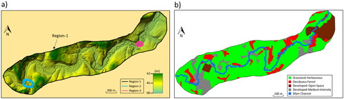
Recognizing the importance of two specific geographical areas for calibration, these were enhanced to improve accuracy: (i) The area of the village of Pensford most affected by the flood, was identified as ‘Region-2’. This region is pivotal for matching the water elevation in our model with historical flood marks from the 1968 event, and it spans an area of 0.034 km² (Figure 4a). (ii) The area around the Compton Dando hydrometric station which provided the observed data, was selected as ‘Region-3’, covering an area of 0.001015 km². The mesh sizes for the Region-1 (Δx_R1), Region-2 (Δx_R2), and Region-3 (Δx_R3) are set to 5 m, 1 m, and 1 m, respectively.

The landcover map presented in Section 2.3 provided comprehensive landcover data required for setup of the HEC-RAS 2D model (Figure 4b). This data enables the specification of Manning’s n values for different land use categories (i.e. five types). Initially, Manning’s n values were set according to the recommendations in the HEC-RAS manual Hydrologic Engineering Center (2023). Subsequently, during the calibration phase, these values were fine-tuned to secure the closest match between the observed and simulated hydrographs at the Compton Dando hydrometric station.

Acknowledging the relatively modest changes in the area of our interest from 1968 to recent times, the initial set up and calibration of the HEC-RAS 2D model was based on the 2023 geometry and recent recorded events. After achieving satisfactory performance in replicating these events numerically, we replaced one of the bridges constructed post-1968 flood reconstructing thus the hydraulic conditions of the river at the time of the flood.

Within the designated study area (Region-1), five bridges cross the River Chew, all of which were incorporated into our model (Figure 5a). The dimensions and associated cross-sections of the bridges were provided by the Environmental Agency through an existing dataset. However, this dataset lacked geo-referencing, prompting our team to conduct a series of field surveys (Figure 5b). These surveys were aimed at determining the precise locations of the dimensions provided for each bridge. Additionally, to guarantee accuracy, the bridges were further surveyed and compared with the existing data. This process ensured precise alignment with the survey locations and verified the accuracy of the crafted DEM. The cross sections derived from the survey closely matched those in the crafted DEM, with a minimal discrepancy of 10–15 cm.

Figure 5. (a) Google map illustrating all five bridges (Bridges-1 to 5) (B-1 to B-5) on the River Chew and marking Pensford village’s position. (b) Field trip for data collection, depicting B-1 and a team member (Ramtin Sabeti) engaged in the measurement process. (c) Historical photograph of the Pensford bridge which collapsed during the 1968 flood (Pensford Local History Group’s ‘Robert Bailey Collection’ (RBC 2096). (d) Detailed profile of B-1 and (e) B-2 in HEC-RAS geometry.

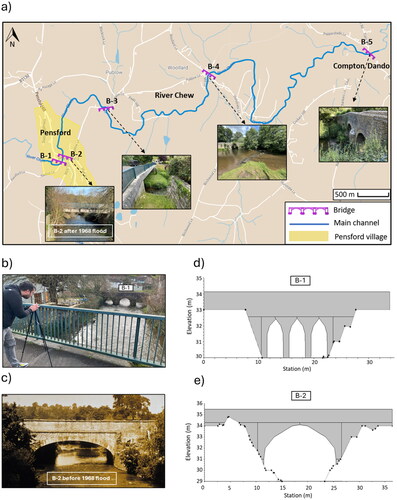
Despite extensive searches, no technical drawings of the original bridge destroyed during the 1968 flood (Figure 5c) were identified, consequently, a series of historical photographs were analysed, utilizing scales such as cars and people present in those photos, to estimate the dimensions of the bridge. Additionally, a historical map from 1950 provided valuable assistance in determining the width of the bridge deck.

In order to effectively simulate bridges within the HEC-RAS 2D, the Google Earth map layer was initially integrated via Ras Mapper to accurately localize each of the bridges. We applied the 'Storage Area/2D Flow Areas connection (SA/2D Conn)' tool in the Geometry section for specific adjustments to bridge components, including piers, sloping abutments, and deck, based on the field survey data. For each bridge, sections both upstream and downstream were defined in the model (Figure 5d,e).

3.2.3. Sensitivity analysis of computational parameters

A series of sensitivity analyses was carried out on key computational parameters of the HEC-RAS 2D model to optimize accuracy and computational efficiency. These analyses included evaluations of mesh size, time step duration, equation types for solving flow routing, and numerical methods. The input hydrograph created from the rainfall event of 20–23 November 2016 (interval = 15 min) by HEC-HMS (Figure 3c), was used for these analyses. At the Compton Dando station, a profile line defined in Ras Mapper provided a simulated hydrograph, enabling direct comparison with observations.

First, a mesh sensitivity analysis in HEC-RAS 2D was undertaken to determine the optimal mesh size. This involved assessing the impact of varying mesh densities on the simulated hydrograph at Compton Dando, specifically examining three distinct mesh sizes as outlined in Table 4. The analysis concluded that the optimal mesh choice is Mesh-1 with grid size of 5 m for the Region-1, and 1 m for the Regions-2 and 3 (Table 4). This combination resulted in the generation of a total of 169,749 computational cells. This choice was guided by observations of a satisfactory level of independence in the results. Specifically, compared to Mesh-2, which has half the grid spacing, the deviation was 1.2% (Figure 6a). This was further supported by a NSC calculation between these two meshes considering the Mesh-1 as the nominal (reference), which indicated an extremely low sensitivity with a value of −0.024. Notably, a mesh size with double the grid spacing of Mesh-1 failed to provide the necessary refinement to adequately minimize errors, as evidenced by a deviation of 7% (Figure 6a); This higher sensitivity was highlighted by the NSC of 0.07 for Mesh-1 and 3.

Figure 6. Sensitivity of numerical simulations to the sizes of (a) the mesh ($\Delta x$), and (b) the time step ($\Delta t$) for HEC-RAS 2D. Dimension of each mesh is presented in Table 4. (c) Sensitivity analysis of nine combinations of solving equations and numerical methods of HEC-RAS 2D in the simulation of the 20–23 November 2016 event. All hydrographs in panels (a), (b) and (c) simulate the flow events in River Chew from 20 to 23 November 2016.

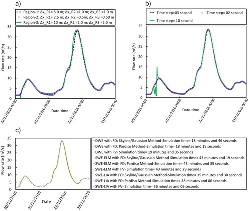
Table 4. Grid size combinations for regions 1, 2, and 3 in mesh sensitivity analysis.

Mesh- No	Region-1, Δx_R1 (m)	Region-2, Δx_R2 (m)	Region-3, Δx_R3 (m)
Mesh-1	5.0	1.0	1.0
Mesh-2	2.5	0.5	0.50
Mesh-3	10	2.0	2.0

Next, the impact of time step duration was considered (Figure 6b). Adhering to the CFL condition, compatibility with both the Shallow Water Equations (C ≤ 1) and the Diffusion-Wave equations (C ≤ 2), was ensured. To determine an appropriate time, step the maximum flow velocity of 1.56 m/s was derived by extracting velocity layers from the HEC-RAS 2D simulation for the event of 20–23 November 2016. Considering that the selected mesh size had a grid spacing (Δx) of 5 m in the major domain of our study area, we conducted an analysis with time steps ranging from 2 to 10 s. The results indicate that using a 10-s time step led to simulation instability, manifesting as a 17% deviation compared to the 2-s time step. Conversely, both 2-s and 3-s intervals demonstrated stability, showing only a 0.5% deviation. Regarding the NSC, the comparison between time steps of 2 s (used as the nominal reference) and 3 s yielded an NSC value of −0.025, indicating minimal sensitivity. However, increasing the time step from 3 s to 10 s markedly increased sensitivity, evidenced by a NSC value of 0.143. This highlights a significant impact on model performance with larger time steps. Consequently, a 3-s time step was selected as optimal.

Finally, a sensitivity analysis was performed on different equation types and numerical methods by varying Computation options and Tolerances provided by HEC-RAS 2D (Figure 6c). The following equation types were considered for this analysis: 1-Wave Equations (DWE) 2-Shallow Water Equations-Eulerian-Lagrangian Method (SWE-ELM) and 3-Shallow Water Equations-Local Inertia Approximation (SWE-LIA). Alongside these, we assessed the following available numerical methods: (i) Skyline/Gaussian method (finite difference), (ii) Pardiso method (finite difference), and (iii) the Finite Volume Method. This exploration resulted in a total of nine unique combinations. For all tests, we used the input hydrograph generated by HEC-HMS for the event of 20–23 November 2023 (Figure 3c). It was observed that all nine combinations of solving equations and numerical methods produced approximately identical output hydrographs. However, there was substantial variation in simulation times across the different methods. For instance, the simulation using DWE with the finite difference Skyline/Gaussian method was completed in 18 min and 46 s, whereas the SWE-LIA method coupled with the finite volume approach required 43 min and 56 s (Figure 6c). In terms of the Normalized Sensitivity Coefficient (NSC), the average NSC for all nine combined equation types and numerical methods was calculated to be 0.015. This calculation focused on the effect of changes in the equation types and numerical methods on the simulated hydrograph. The reference test utilized the DWE as the solving equation and Skyline/Gaussian as the numerical method. An NSC value of 0.015 indicates that the model output is minimally sensitive to these changes. Based on these results it was decided that the combination of DWE as the solving equations and Skyline/Gaussian as the numerical method was the most effective setup for our simulations, optimizing both accuracy and computational efficiency. It is important to note that all simulations, using Mesh-1 with a 3-s time step, were conducted on a PC configured with an Intel^® Core^™ i7-8700 CPU (3.20 GHz) and 32 GB of RAM.

3.2.4. Calibration of HEC-RAS 2D

Calibration of the HEC-RAS 2D model was focused on three distinct events: (1) 7–13 December 2017; (2) 20–23 November 2016; and (3) 28 April–1 May 2012 (Figure 7). For each event, the input hydrographs were obtained from the calibrated HEC-HMS model at Junction-2, situated at the upstream boundary of HEC-RAS model. The output hydrographs and water depths simulated by HEC-RAS were then compared with the observations at the Compton Dando hydrometric station as per Equation 1(1) $$\epsilon =\left|\frac{O_i-S_i}{O_i}\right|\times 100$$(1) . The choice of these events, all post-2011, was dictated by the operational commencement of the Chew Magna rain gauge station in 2011. The results indicated that there was an average flow rate simulation mismatch of 30% compared to observed values, and a 34% mismatch in water depths (Figure 7). To calculate the mismatch error, initial zero values recorded in simulations prior to the flow reaching the gauge station were removed from the calculations (Equation 1(1) $$\epsilon =\left|\frac{O_i-S_i}{O_i}\right|\times 100$$(1) ). The Manning’s n values were adjusted across five land use categories, as delineated by the landcover data, to achieve the best match (Table 5) comparing simulated hydrographs and water depths for the three events of 2012, 2016 and 2017. For the events of 2012, 2016, and 2017, we configured the warm-up and ramp-up periods as follows: 10 h and 1 h for the events of 2016 and 2017, respectively, and 18 h and 1.8 h for the event of 2012.

Figure 7. Comparison of observed and modelled hydrographs and water depths from HEC-RAS 2D for events at Compton Dando station: (a) hydrograph for December/2017, (b) Water depth for December/2017, (c) Hydrograph for November/2016, (d) Water depth for November/2016, (e) Hydrograph for April/2012, and (f) Water depth for April/2012.

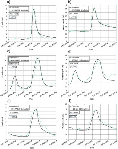
Table 5. Manning’s n values for various landcover types and main channel of the River Chew in the Region-1 (Figure 4b).

Landcover Type	Manning’s n value
Grassland-Herbaceous	0.065
Deciduous Forest	0.085
Developed- Open Space	0.050
Developed-Medium Intensity	0.130
Main Channel	0.045

3.3. Digitizing hydrograph of 1968 event

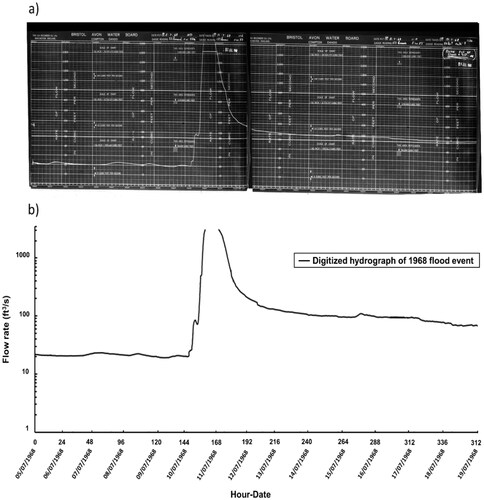
Due to the unavailability of detailed rainfall data during the 1968 event, it was decided to apply the observed hydrograph of the 1968 flood event, which was recorded at the Compton Dando station, see Figure 8. This data serves as the upstream boundary condition for our HEC-RAS model. The microfilm containing this hydrograph was found in the archives of the National River Flow Archive (NRFA) in Wallingford. The hydrograph from the 1968 flood event, digitized using WebPlotDigitizer, was adopted as the primary input for the HEC-RAS 2D hydraulic model. This study specifically considers the well-recorded rising and falling limbs of the hydrograph, each peaking at approximately 3000 ft³/s (∼85 m³/s), which have been verified with continuous, uninterrupted data records. These segments were implemented directly in the hydrological model as confirmed data. Conversely, the peak section of the hydrograph, which lacks recorded data possibly due to equipment limitations at the time of the event, was estimated. Using a reverse engineering methodology, detailed further in the Results and discussions section, we ascertained the most probable hydrograph associated with the 1968 event.

Figure 8. (a) The recorded 1968 hydrograph on microfilm at Compton Dando station, illustrating river flow data (flow rate and water depth) from 5th to 19th july 1968. (b) Corresponding digitized hydrograph, representing the data transformation from the original records.

4. Results and discussions

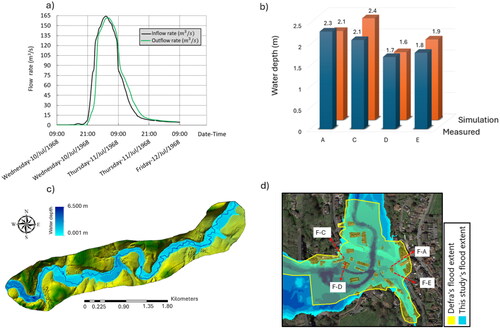
Through a reverse engineering process, we estimated the peak of the 1968 flood event hydrograph, beginning with the confirmed value of 85 m³/s and adjusting to higher peak values. This analysis was confined to the period from July 10th to 12th, corresponding with the flash flood, to avoid simulating unnecessary parts of the hydrograph and reduce the simulation time. Every estimated hydrograph was fed into our calibrated HEC-RAS 2D model as the input of the upstream boundary. Subsequently, we compared the water depth simulation results with the measured water depths at the locations of the six flood marks labelled A, B, C, D, E, and F (Table 2). By comparing the modelled water depths to the flood marks, noticeable discrepancies were observed at flood marks B and F, more pronounced than at the other flood marks. Since flood mark F was located inside a building, and HEC-RAS simulated the building as an impermeable block preventing water from entering, it was decided to exclude this point from the analysis. However, it serves as corroborative evidence for flood marks A and E, which are situated around this building. Consequently, we decided to concentrate our analysis on flood marks A, C, D and E. The most accurate match between the simulated water depths and flood marks was achieved with an input hydrograph with a peak flow of 165 m³/s (Figure 9a); This figure illustrates the output hydrograph generated by HEC-RAS 2D at Compton Dando, showing a decrease of about 4 m³/s from the upstream input hydrograph. This reduction is attributed to the spatial flood spread between the upstream and downstream boundaries. The average difference between simulations for the four flood marks (A, C, D, and E) and the observed values was about 8.6%, as depicted in Figure 9b. While this provides an indication of the model’s performance at specific locations, it is important to note that this accuracy might not fully represent the entire hydrograph. Given the inherent complexities and uncertainties in flood modelling, we estimate the potential error in the simulated hydrograph to be around 8.6%, with the understanding that actual errors may vary spatially and temporally. These uncertainties arise from various sources, including the precision of historical data, the spatial and temporal resolution of our DEM, and the simplifications necessary for computational modelling. As such, while the results present a scientifically informed estimate of flood behaviour, they should not be interpreted as absolute predictions. This nuanced understanding highlights the importance of adopting a cautious and adaptive approach in using these findings for planning and decision-making processes, acknowledging the probabilistic nature of flood risk assessment and the ever-present need for further research.

Figure 9. (a) Input hydrograph from 1968’s digitized flow data, manually augmented with a peak, compared to the output hydrograph at Compton Dando by HEC-RAS 2D. (b) Water depth layer for Region-1 from the 1968 event simulation, overlaid on the crafted DEM base map. (c) Comparison of flood extent in this study with Defra’s assessment. (d) Comparison of simulated water depths against observed flood mark levels. Parameters: F = Flood mark.

It is important to note that the available rating curve for at Compton Dando station (provided by NRFA) has a maximum capacity of 100 m³/s. However, our estimated flood magnitude for the 1968 event is 165 m³/s. This significant discrepancy indicates that the existing rating curve is not capable of accurately representing the peak flow of this historical flood event. The limitations of the rating curve in this context are due to its inability to accommodate flows beyond 100 m³/s.

The flood extent simulated by HEC-RAS 2D in the Region-1 area, highlighting that the maximum water depth reached higher than 6 meters around Region-2, is shown in Figure 9c. Our flood extent layer, detailing the water depth in Pensford, is compared with a historical flood map provided by Defra, which presents the maximum flood extent layer (https://www.data.gov.uk/dataset/76292b-/historic-flood-map) (Figure 9d). This Defra layer vividly illustrates the maximum boundaries of individual recorded flood outlines from the river, spanning a period from 1946 to February 2024 (Figure 9d). This analysis reveals a high degree of agreement regarding the flood extent area between our study and the flood extent layer presented by Defra, which confirms our results. Quantitatively, the area presented by our study and the area presented by Defra matches approximately 78%. Furthermore, we applied NSE (Equation 4(4) $$\mathit{\text{NSE}}=1-\frac{\sum _{i=1}^n{\left(D_{\mathit{\text{obs}},i}-D_{\mathit{\text{sim}},i}\right)}^2}{\sum _{i=1}^n{\left(D_{\mathit{\text{obs}},i}-{\overline{D}}_{\mathit{\text{obs}}}\right)}^2}$$(4) ) and PBIAS (Equation 5(5) $$\mathit{\text{PBIAS}}=\left(\frac{{\sum }_{i=1}^n\left(D_{\mathit{\text{obs}},i}-D_{\mathit{\text{sim}},i}\right)}{{\sum }_{i=1}^n\left(D_{\mathit{\text{obs}},i}\right)}\right)\times 100$$(5) ) metrics to further evaluate the performance of our results (i.e. water depths). The NSE is calculated to be 0.66, indicating that the simulations have a fair level of accuracy in capturing the variability of the observed data, considering the high uncertainties involved. The Percent Bias (PBIAS) is −1.27%, showing that the model has a slight tendency to overestimate the observed values.

The reconstructed peak discharge of the 1968 flood, with an estimation of 165 m³/s carrying a degree of uncertainty, suggests important considerations. Hydrological models could require recalibration, which might improve the accuracy of future flood predictions and might suggest a shorter return period for high-magnitude floods. Additionally, understanding the extent of the 1968 flood could inform environmental impact assessments, aiding current environmental conservation strategies.

These new results can inform the development of nature-based solutions, such as green infrastructure e.g. wetlands and urban forests, which help in mitigating flood risks by improving water absorption and delaying runoff. These nature-based solutions represent potential environmentally friendly options nevertheless are not the only solutions.

Incorporating these findings into community planning and emergency management strategies could also enhance resilience. Lastly, this updated peak discharge information provides an opportunity for further research into frequency analyses and risk assessment, which are crucial for understanding and addressing the potential impacts of future flood events.

5. Conclusion

A detailed study of the hydrology and hydraulics of the River Chew and its catchment has been conducted in an attempt to reconstruct the 1968 flood event. Initial step involved gathering data from existing reports, literature, newspapers, and organizing a community workshop to collect eyewitness accounts from locals who remembered the event. We setup and calibrated hydrological (HEC-HMS) and hydraulic (HEC-RAS 2D) models using contemporary data, including a crafted DEM, land cover map, and the most fitting Manning’s values to replicate the observed flow rates at Compton Dando. Adapting this validated model to the 1968 landscape and hydraulic conditions, we used a digitized hydrograph from the 1968 records at Compton Dando as the input hydrograph. Through a reverse engineering approach, we adjusted a series of input hydrographs, all based on the digitized 1968 data, incrementally increasing the hydrograph’s peak until the simulated water depths matched the observed flood marks. The main conclusions are:

• Despite prevailing uncertainties, our analysis suggests that the peak flow of the hydrograph was 165 m³/s. This is higher than the official estimate of 100 m³/s, representing a 65% increase.

• A HEC-RAS 2D unsteady model was calibrated using three events for the areas covering Pensford and Compton Dando. The average mismatch errors between observed flow rates and water depths and their simulated values were 30% and 34%, respectively.

• The maximum water depth during the 1968 event reached approximately 6.5 meters, with the flood extent covering an area of 0.94 km².

• The methodological framework developed in this study can be applied to reconstruct historical flash flood events in other regions, making it a valuable tool for researchers and flood managers worldwide. This is particularly important for areas with limited historical or field data or flash flood-prone regions.

• The reconstructed peak discharge of the 1968 Pensford flood, while accompanied by a certain level of uncertainty, proposes potential updates to flood hazard maps, recalibration of hydrological models, and revised risk assessments, suggesting the importance of considering nature-based solutions and informing long-term river management strategies.

Our research offers innovative insights into the hydrology and hydraulic characteristics of an unpredicted flash flood by integrating historical data with advanced numerical modelling. This study sets a new benchmark for researchers aiming to investigate flash flood events, providing a robust framework and novel methodologies for future explorations. The significance of these findings will greatly influence the overall assessment of the current flood risk for both the River Chew and the wider region. It is likely that current estimates of flood risk could be underestimated. However, it is also important to acknowledge that the reconstruction involves uncertainties from a number of different sources, including model limitations as well as uncertainty in the historical data. These uncertainties and their influence on the reconstructed peak flow value should be quantified before a more comprehensive re-evaluation of the local regional flood risk should be attempted based on these results.

Acknowledgements

The authors are grateful to the members of the Pensford Local History Group and the wider community of the Chew Valley for their support and invaluable contribution to the data collection efforts. The Environment Agency, the National River Flow Archive, and UK Centre for Ecology and Hydrology provided access to river geometry, flow data and landcover map. The work was kindly funded by a Leverhulme Trust Research Project Grant.

Disclosure statement

The authors declare that they have no known competing financial interests or personal relationships that could have appeared to influence the work reported in this paper.

Data availability statement

All data used in this study are either open-access or given in the body of the article.

Additional information

Funding

This work was supported by the Leverhulme Trust project grant: RPG-2022-306.

References

- Bartl S, Schümberg S, Deutsch M. 2009. Revising time series of the Elbe River discharge for flood frequency determination at gauge Dresden. Nat Hazards Earth Syst Sci. 9(6):1805–1814. doi: 10.5194/nhess-9-1805-2009.
- Benito G, Lang M, Barriendos M, Llasat MC, Francés F, Ouarda T, Thorndycraft V, Enzel Y, Bardossy A, Coeur D, et al. 2004. Use of systematic, palaeoflood and historical data for the improvement of flood risk estimation. Review of scientific methods. Natural Hazards. 31(3):623–643. doi:10.1023/B:NHAZ.0000024895.48463.eb.
- Brunner GW. 2016. HEC-RAS river analysis system: hydraulic reference manual, Version 5.0. US Army Corps of Engineers–Hydrologic Engineering Center. 547.
- Brunner GW. 2018. Benchmarking of the HEC-RAS two-dimensional hydraulic modelling capabilities. Davis, CA: US Army Corps of Engineers, p. 1–137.
- Benito G, Ballesteros-Cánovas JA, Díez-Herrero A. 2023. Paleoflood hydrology: reconstructing rare events and extreme flood discharges. In: Paron P, Di Baldassarre G, editors. Hydro-Meteorol. Hazards Risks Disasters. Amsterdam, Netherlands: Elsevier; p. 33–83. https://doi.org/10.1016/B978-0-12-819101-9.00009-1.
- Cahyono AB, Hak AB. 2023. Flood inundation simulation using HEC-GeoRAS with Hydro-Enforced-DTM LiDAR Data. IOP Conf Ser: Earth Environ Sci. 1127(1):012049. IOP Publishing. doi:10.1088/1755-1315/1127/1/012049.
- Elleder L, Herget J, Roggenkamp T, Nießen A. 2013. Historic floods in the city of Prague–a reconstruction of peak discharges for 1481–1825 based on documentary sources. Hydrol. Res. 44(2):202–214. doi:10.2166/nh.2012.161.
- Ghimire E, Sharma S, Lamichhane N. 2022. Evaluation of one-dimensional and two-dimensional HEC-RAS models to predict flood travel time and inundation area for flood warning system. ISH J. Hydraul. Eng. 28(1):110–126. doi:10.1080/09715010.2020.1824621.
- González-Cao J, Fernández-Nóvoa D, García-Feal O, Figueira JR, Vaquero JM, Trigo RM, Gómez-Gesteira M. 2021. Numerical reconstruction of historical extreme floods: the Guadiana event of 1876. J. Hydrol. 599:126292. doi:10.1016/j.jhydrol.2021.126292.
- Hand WH, Fox NI, Collier CG. 2004. A study of twentieth-century extreme rainfall events in the United Kingdom with implications for forecasting. Meteorol Appl. 11(1):15–31. doi:10.1017/S1350482703001117.
- Huo AD, Guan WK, Dang J, Wu TZ, Shantai H, Wang W, Liew MWV. 2016. Submerged area of typical torrential flood and debris-flow disasters in Mengzong Gully, China. Geomatics Nat Hazards Risk. 7(sup1):18–24. doi:10.1080/19475705.2016.1181340.
- Hydrologic Engineering Center. 2023. HEC-RAS User’s Manual (Version 6.4.1). Davis CA: U.S. Army Corps of Engineers.
- Kjeldsen TR, Macdonald N, Lang M, Mediero L, Albuquerque T, Bogdanowicz E, Brázdil R, Castellarin A, David V, Fleig A, et al. 2014. Documentary evidence of past floods in Europe and their utility in flood frequency estimation. J Hydrol. 517:963–973., doi:10.1016/j.jhydrol.2014.06.038.
- Lucas M, Renard B, Le Coz J, Lang M, Bard A, Pierrefeu G. 2023. Are historical stage records useful to decrease the uncertainty of flood frequency analysis? A 200-year long case study. J Hydrol. 624:129840. doi: 10.1016/j.jhydrol.2023.129840.
- Mancini CP, Lollai S, Calenda G, Volpi E, Fiori A. 2022. Guidance in the calibration of two-dimensional models of historical floods in urban areas: a case study. Hydrol Sci J. 67(3):358–368. doi:10.1080/02626667.2021.2022153.
- Mehta DJ, Eslamian S, Prajapati K. 2022a. Flood modelling for a data-scare semi-arid region using 1-D hydrodynamic model: a case study of Navsari Region. Model Earth Syst Environ. 8(2):2675–2685. doi:10.1007/s40808-021-01259-5.
- Mehta DJ, Kumar YV. 2022b. Flood Modelling Using HEC-RAS for Purna River, Navsari District, Gujarat, India. Water Resour. Manag. Sustain. 2022:213–220.
- Moriasi, D.N., Arnold, J.G., Van Liew, M.W., Bingner, R.L., Harmel, R.D. and Veith, T.L., 2007. Model evaluation guidelines for systematic quantification of accuracy in watershed simulations. Transactions of the ASAB. 50(3): 885–900. doi:10.13031/2013.23153.
- Marston C, Rowland CS, O’Neil AW, Morton RD. 2022. Land Cover Map 2021. UK: NERC EDS Environmental Information Data Centre. doi: 10.5285/a1f85307-cad7-4e32-a445-84410efdfa70.
- Mishra SK, Singh V. 2003. Soil conservation service curve number (SCS-CN) methodology. Vol. 42. Dordrecht, Netherlands: Springer Science and Business Media. https://link.springer.com/book/10.1007/978-94-017-0147-1
- Niaz A, Nisar UB, Khan S, Faiz R, Javed A, Niaz J, Aaqib M, Raza M, Bhusal B. 2023. Flood modelling and its impacts on groundwater vulnerability in sub-Himalayan region of Pakistan: integration between HEC-RAS and geophysical techniques. Geomatics Nat Hazards Risk. 14(1):2257360. doi:10.1080/19475705.2023.2257360.
- Ngo H, Bomers A, Augustijn DC, Ranasinghe R, Filatova T, van der Meulen B, Herget J, Hulscher SJ. 2023. Reconstruction of the 1374 Rhine River flood event around Cologne region using 1D-2D coupled hydraulic modelling approach. J. Hydrol. 617:129039. doi:10.1016/j.jhydrol.2022.129039.
- Pekárová P, Halmová D, Mitková VB, Miklánek P, Pekár J, Škoda P. 2013. Historic flood marks and flood frequency analysis of the Danube River at Bratislava, Slovakia. J. Hydrol. Hydromech. 61(4):326–333. doi:10.2478/johh-2013-0041.
- Prosdocimi I. 2018. German tanks and historical records: the estimation of the time coverage of ungauged extreme events. Stoch Environ Res Risk Assess. 32(3):607–622. doi:10.1007/s00477-017-1418-8.
- Salter PRS. 1968. An exceptionally heavy rainfall in July 1968. Meteorol. Mag. 97:372–380.
- Sabeti R, Heidarzadeh M, Romano A, Ojeda G, Lara L. 2024. Three-dimensional simulations of subaerial landslide-generated Waves: comparing OpenFOAM and flow-3D Hydro Models. Pure Appl Geophys. 181(4):1075–1093. doi:10.1007/s00024-024-03443-x.
- Stamataki I, Kjeldsen TR. 2021. Reconstructing the peak flow of historical flood events using a hydraulic model: the city of Bath, United Kingdom. J. Flood Risk Manag. 14(3):e12719.
- Stedinger JR, Vogel RM, Foufoula-Georgiou E. 1993. Frequency analysis of extreme events. In: Maidment DR, editor. Handbook of Hydrology. New York: McGraw-Hill.
- Thomas C, Stamataki I, Rosselló-Geli J. 2023. Reconstruction of the 1974 flash flood in Sóller (Mallorca) using a hydraulic 1D/2D model. J. Hydrol. Hydromech. 71(1):49–63. doi:10.2478/johh-2022-0027.
- Thomas H, Nisbet TR. 2016. Slowing the flow in Pickering: quantifying the effect of catchment woodland planting on flooding using the soil conservation service curve number method. IJSSE. 6:12–20.
- Yang Y, Ma Y, Liu J, Liu B, Du J, He S. 2023. Evaluating the double-kernel smoothing technique of blending TRMM and gauge data to identify flood events in the Xiangjiang River Basin, China. Geomatics Nat Hazards Risk. 14(1):2221991. doi:10.1080/19475705.2023.2221991.
- Yoon J, Padmanabhan G. 1993. Parameter estimation of linear and nonlinear Muskingum models. J Water Resour Plann Manage. 119(5):600–610. doi: 10.1061/(ASCE)0733-9496(1993)119:5(600).